32
128 Slides for “Wireless Communications” © Edfors, Molisch, Tufvesson Chapter 6 Wideband channels

Chapter 6sce.uhcl.edu/goodwin/ceng5332/downloads/chapter_6.pdfNarrowband versus Wideband Systems. Delay Spread\rmuch less than\rsymbol period. These diagrams show the time domain and

  • Upload
    vuhuong

  • View
    215

  • Download
    1

Embed Size (px)

Citation preview

128Slides for “Wireless Communications” © Edfors, Molisch, Tufvesson

Chapter 6

Wideband channels

Kenneth
Typewritten Text
Delay Dispersion - the arriving signal has a longer duration than the transmitting signal (the impulse response of the channel is not a delta function). This is the same as the channel transfer function changing over the bandwidth of interest (the frequency selectivity of the channel not being constant). Wideband channels are required for multiple access and/or high data rates.
krgoodwin
Typewritten Text
Chapter 5 covered narrowband channels where the transmit signal was a pure sinusoid.

129Slides for “Wireless Communications” © Edfors, Molisch, Tufvesson

Delay (time) dispersion

A simple case

Transmitted impulse Received signal

(channel impulse response)

h

1 1 2 2 3 3h a a a

1

1a

2

2a

33a

Kenneth
Typewritten Text
Impulse Response of the Channel
Kenneth
Typewritten Text
Kenneth
Typewritten Text
Kenneth
Typewritten Text
Kenneth
Typewritten Text
Kenneth
Typewritten Text
(delta function)
Kenneth
Typewritten Text
krgoodwin
Typewritten Text
Received signal shows delay dispersion in the time domain leading to ISI yet less impact than from fading
krgoodwin
Typewritten Text
krgoodwin
Typewritten Text
krgoodwin
Typewritten Text
krgoodwin
Typewritten Text
krgoodwin
Typewritten Text
see Figure 6.1 for transfer function in the Frequency Domain with deep nulls
krgoodwin
Typewritten Text
krgoodwin
Typewritten Text
krgoodwin
Typewritten Text
krgoodwin
Typewritten Text

130Slides for “Wireless Communications” © Edfors, Molisch, Tufvesson

Delay (time) dispersion

One reflection/path, many paths

2 3 4 0

“Impulse

response”

Delay in excess

of direct path

Kenneth
Typewritten Text
Delay dispersion in the time domain (t) translates into frequency selectivity in the frequency domain (f). Group responses into same 'bin' and use equations from Chapter 5 for each delay bin.
Kenneth
Typewritten Text
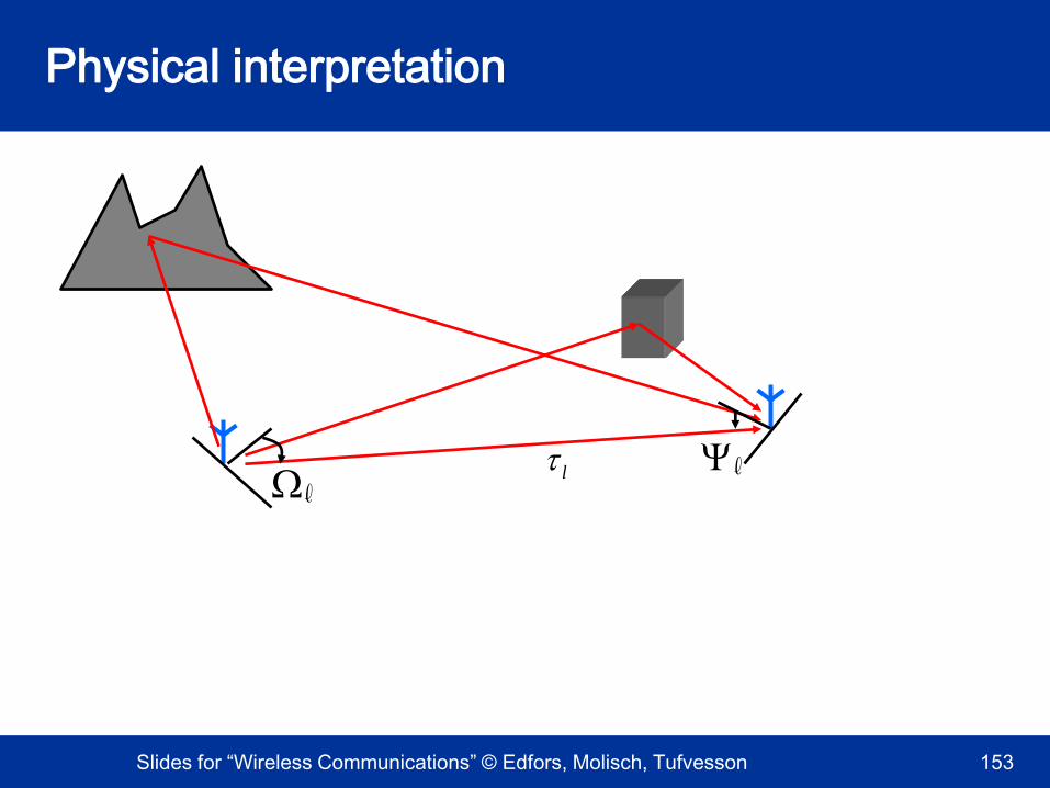
More generalized case versus the simple two-path model of Chapter 5
Kenneth
Typewritten Text
Kenneth
Typewritten Text
Kenneth
Typewritten Text
Signals that interact with objects on the same ellipse (red, blue, etc.) arrive at the RX at the same time
Kenneth
Typewritten Text
Kenneth
Typewritten Text
Kenneth
Typewritten Text
Kenneth
Typewritten Text
Kenneth
Typewritten Text
Kenneth
Typewritten Text
Kenneth
Typewritten Text
Kenneth
Typewritten Text
Kenneth
Typewritten Text
Kenneth
Typewritten Text
krgoodwin
Typewritten Text
krgoodwin
Typewritten Text
krgoodwin
Typewritten Text
krgoodwin
Typewritten Text
krgoodwin
Typewritten Text
krgoodwin
Typewritten Text
krgoodwin
Typewritten Text
krgoodwin
Typewritten Text
krgoodwin
Typewritten Text
krgoodwin
Typewritten Text
krgoodwin
Typewritten Text
krgoodwin
Typewritten Text
krgoodwin
Typewritten Text
krgoodwin
Typewritten Text
krgoodwin
Typewritten Text
krgoodwin
Typewritten Text
krgoodwin
Typewritten Text
krgoodwin
Typewritten Text
krgoodwin
Typewritten Text
krgoodwin
Typewritten Text
krgoodwin
Typewritten Text
krgoodwin
Typewritten Text
krgoodwin
Typewritten Text
krgoodwin
Typewritten Text
krgoodwin
Typewritten Text
krgoodwin
Typewritten Text
krgoodwin
Typewritten Text
krgoodwin
Typewritten Text
krgoodwin
Typewritten Text
Narrowband versus Wideband Systems
krgoodwin
Typewritten Text
krgoodwin
Typewritten Text
krgoodwin
Typewritten Text
krgoodwin
Typewritten Text
krgoodwin
Typewritten Text
krgoodwin
Typewritten Text
krgoodwin
Typewritten Text
krgoodwin
Typewritten Text
krgoodwin
Typewritten Text
Delay Spread much less than symbol period
krgoodwin
Typewritten Text
krgoodwin
Typewritten Text
krgoodwin
Typewritten Text
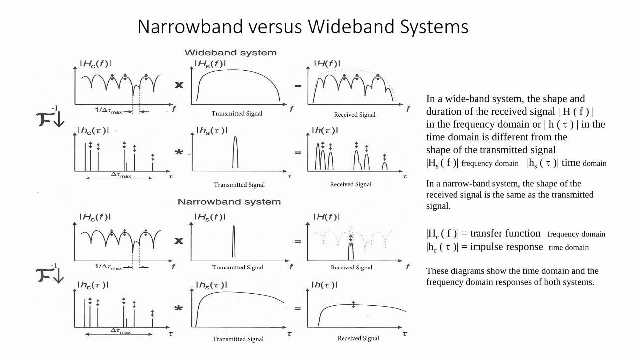
These diagrams show the time domain and the frequency domain responses of both systems. In the wideband system, the shape and duration of the received signal R(f) in the frequency domain or r(t) in the time domain is different from the shape of the transmitted signal. The channel is frequency selective as shown in H(f) and the channel induces intersymbol interference (ISI). In the narrowband system or flat fading as shown in H(f), the spectral characteristics of transmitted signal are preserved although the gain of the channel gain changes over time caused by multipath and best described by a Rayleigh distribution.
krgoodwin
Typewritten Text
krgoodwin
Typewritten Text
krgoodwin
Typewritten Text
Narrowband System
krgoodwin
Typewritten Text
krgoodwin
Typewritten Text
krgoodwin
Typewritten Text
krgoodwin
Typewritten Text
krgoodwin
Typewritten Text
Wideband System
krgoodwin
Typewritten Text
krgoodwin
Typewritten Text
krgoodwin
Typewritten Text
Time Domain
krgoodwin
Typewritten Text
Time Domain
krgoodwin
Typewritten Text
krgoodwin
Typewritten Text
Frequency Domain
krgoodwin
Typewritten Text
Frequency Domain
krgoodwin
Typewritten Text
krgoodwin
Typewritten Text
krgoodwin
Typewritten Text
krgoodwin
Typewritten Text
krgoodwin
Typewritten Text
krgoodwin
Typewritten Text
krgoodwin
Typewritten Text
krgoodwin
Typewritten Text
krgoodwin
Typewritten Text
Transmitted Signal
krgoodwin
Typewritten Text
krgoodwin
Typewritten Text
Received Signal
krgoodwin
Typewritten Text
krgoodwin
Typewritten Text
Channel
krgoodwin
Typewritten Text

Narrowband versus Wideband Systems

In a wide-band system, the shape and

duration of the received signal | H ( f ) |

in the frequency domain or | h ( t ) | in the

time domain is different from the

shape of the transmitted signal

|Hs ( f )| frequency domain |hs ( t )| time domain

In a narrow-band system, the shape of the

received signal is the same as the transmitted

signal.

|Hc ( f )| = transfer function frequency domain

|hc ( t )| = impulse response time domain

These diagrams show the time domain and the

frequency domain responses of both systems.

Transmitted Signal

Transmitted Signal

Received Signal

Received Signal

Transmitted Signal

Transmitted Signal

Received Signal

Received Signal-1

-1

132Slides for “Wireless Communications” © Edfors, Molisch, Tufvesson

2B

1B

Narrow- versus wide-band

Channel frequency response

|dB

H f

f

krgoodwin
Typewritten Text
Narrowband: transfer function is not frequency dependent which can be described by a single attenuation coefficient - a constant Wide-band: details of the transfer function must be modeled (large variations as shown)
krgoodwin
Typewritten Text
Narrowband - blue signal Wideband - wide pink area Channel transfer function in the frequency domain - red
krgoodwin
Typewritten Text
krgoodwin
Typewritten Text

133Slides for “Wireless Communications” © Edfors, Molisch, Tufvesson

System functions (1)

• Time-variant impulse response

– Due to movement, impulse response changes with time

– Input-output relationship:

• Time-variant transfer function H(t,f)

– Perform Fourier transformation with respect to

– Input-output relationship

becomes Y(f)=X(f)H(f) only in slowly time-varying channels

ht,

yt

xt ht,d

Ht, f

ht,expj2fd

Yf

XfHt, fexpj2ftexpj2

f tdfdt

Kenneth
Typewritten Text
h( ) completely characterizes the channel and is a function of 2 variables: time and delay --> LTV
Kenneth
Typewritten Text
Kenneth
Typewritten Text
Kenneth
Typewritten Text
Kenneth
Typewritten Text
Kenneth
Typewritten Text
Kenneth
Typewritten Text
Kenneth
Typewritten Text
Kenneth
Typewritten Text
h (time, delay)
Kenneth
Typewritten Text
Kenneth
Typewritten Text
Kenneth
Typewritten Text
Kenneth
Typewritten Text
Kenneth
Typewritten Text
Kenneth
Typewritten Text
Kenneth
Typewritten Text
LTI theory applies with minor mods
krgoodwin
Typewritten Text
Output signal = input signal multiplied by the spectrum of the currently valid transfer function (quasi static system)
krgoodwin
Typewritten Text
krgoodwin
Typewritten Text
krgoodwin
Typewritten Text
krgoodwin
Typewritten Text
krgoodwin
Typewritten Text
krgoodwin
Typewritten Text

134Slides for “Wireless Communications” © Edfors, Molisch, Tufvesson

Transfer function, Typical urban

Kenneth
Typewritten Text
For a simpler representation of a two path model's transfer function - Fig 6.1 pg 103 Fig 6.2 pg 103 shows that the group delay (d/dt of the phase) is very large at the fading dips in the transfer function.

135Slides for “Wireless Communications” © Edfors, Molisch, Tufvesson

System functions (2)

• Further equivalent system functions:

– Since impulse response depends on two variables, Fourier

transformation can be done w.r.t. each of them

-> four equivalent system descriptions are possible:

• Impulse response

• Time-variant transfer function

• Spreading function

• Doppler-variant spreading function

S,

ht,expj2tdt

B, f

S,expj2fd

Kenneth
Typewritten Text
Kenneth
Typewritten Text
Kenneth
Typewritten Text
Kenneth
Typewritten Text
Kenneth
Typewritten Text
H(t,f) - Fourier transform of impulse response wrt tau
Kenneth
Typewritten Text
Kenneth
Typewritten Text
Kenneth
Typewritten Text
Kenneth
Typewritten Text
Kenneth
Typewritten Text
two variables time and tau (delay)

Wireless Channels – Interrelation BetweenDeterministic System Functions

Time variantimpulse response

Doppler variantImpulse response -spreading functionS(Doppler, delay)

Time variantTransfer function

Doppler variant transfer functionB(Doppler shift, frequency)

Fourier Transformwrt t (delay)

Fourier Transformwrt t (delay)

Fourier Transformwrt t (time)

Fourier Transformwrt t (time)

krgoodwin
Typewritten Text
krgoodwin
Typewritten Text
krgoodwin
Typewritten Text
krgoodwin
Typewritten Text
krgoodwin
Typewritten Text
krgoodwin
Typewritten Text
krgoodwin
Typewritten Text
krgoodwin
Typewritten Text
krgoodwin
Typewritten Text
krgoodwin
Typewritten Text
krgoodwin
Typewritten Text
krgoodwin
Typewritten Text
krgoodwin
Typewritten Text
krgoodwin
Typewritten Text
krgoodwin
Typewritten Text
krgoodwin
Typewritten Text
krgoodwin
Typewritten Text
krgoodwin
Typewritten Text
krgoodwin
Typewritten Text
krgoodwin
Typewritten Text
krgoodwin
Typewritten Text
krgoodwin
Typewritten Text
krgoodwin
Typewritten Text
krgoodwin
Typewritten Text
krgoodwin
Typewritten Text
krgoodwin
Typewritten Text
krgoodwin
Typewritten Text

136Slides for “Wireless Communications” © Edfors, Molisch, Tufvesson

Stochastic system functions

• ACF - autocorrelation function (second-order statistics)

• Input-output relationship:

Rht, t ,, Eht,ht ,

Ryyt, t

Rxxt , t Rht, t ,,dd

Exam physical properties of the channel --> simplify correlation function --> WSS (Wide-Sense Stationary) + US (Uncorrelated scatters --> assumptions lead to WSSUS Model

Kenneth
Typewritten Text
Autocorrelation function (ACF) of the received signal is a combination of the ACF of the transmit signal & the ACF of the channel
Kenneth
Typewritten Text
The autocorrelation function describes the relationship between the second-order moments of the amplitude pdf of the signal y at different times and if the pdf is zero-mean Gaussian, then the 2nd order description contains all the required information of the channel and received signal.
Kenneth
Typewritten Text
Kenneth
Typewritten Text
Note: the ACF of the channel depends on 4 variables
krgoodwin
Typewritten Text
krgoodwin
Typewritten Text
krgoodwin
Typewritten Text
krgoodwin
Typewritten Text
Trying to make things simple
krgoodwin
Typewritten Text
krgoodwin
Typewritten Text
krgoodwin
Typewritten Text

137Slides for “Wireless Communications” © Edfors, Molisch, Tufvesson

The WSSUS model: mathematics

• If WSSUS is valid, ACF depends only on two variables

(instead of four)

• ACF of impulse response becomes

• ACF of transfer function

• ACF of spreading function

Rht, t t,, Pht,

Pht,....Delay cross power spectral density

RHt t, f f RHt,f

Rs,,, Ps,

Ps,.......Scattering function

Wide-Sense Stationary (WSS) assumption depends only on the differences int - t' where the statistical properties of the channel don't change with time.

Fading still a dynamic factor, just the statistics are stationary which leads to aquasi-stationary environment over a time interval (movement of less than 10 λ).

Uncorrelated Scatters (US) assumption depends on differences in frequency. Not truly valid in an indoor environment where for example scatters off a wall are correlated.

Thus WSSUS assumptions more applicable to the outdoors . Popular model (WSSUS) assumptions but not necessarily valid.

Digital Representation – WSSUS Model

138Slides for “Wireless Communications” © Edfors, Molisch, Tufvesson

Condensed parameters

• Correlation functions depend on two variables

• For concise characterization of channel, we desire

– A function depending on one variable or

– A single (scalar) parameter

• Most common condensed parameters

– Power delay profile

– Rms delay spread

– Coherence bandwidth

– Doppler spread

– Coherence time

Kenneth
Typewritten Text
Kenneth
Typewritten Text
even better
krgoodwin
Typewritten Text
krgoodwin
Typewritten Text
(still a cumbersome representation)
krgoodwin
Typewritten Text
krgoodwin
Typewritten Text
krgoodwin
Typewritten Text
krgoodwin
Typewritten Text
krgoodwin
Typewritten Text
integrate over one variable --> single variable
krgoodwin
Typewritten Text
integrate the scattering function over the Doppler shift --> how much power arrives at the RX within a bounded delay
krgoodwin
Typewritten Text
krgoodwin
Typewritten Text
krgoodwin
Typewritten Text
How much info is lost? Acceptable?
krgoodwin
Typewritten Text
krgoodwin
Typewritten Text
krgoodwin
Typewritten Text
Bcoh A better measure for OFDM
krgoodwin
Typewritten Text
Tcoh How fast a channel changes

140Slides for “Wireless Communications” © Edfors, Molisch, Tufvesson

Channel measures

Copyright: Shaker

141Slides for “Wireless Communications” © Edfors, Molisch, Tufvesson

Condensed parameters

Power-delay profile

One interesting channel property is the power-delay profile (PDP),

which is the expected value of the received power at a certain delay:

2

E ,tP h t

Et denotes

expectation

over time.

2

1

2 2

1 1

E exp

E 2

N

t i i i

i

N N

t i i i i

i i

P t j t

t

For our tapped-delay line we get:

Average power of tap i.

142Slides for “Wireless Communications” © Edfors, Molisch, Tufvesson

Condensed parameters

Power-delay profile (cont.)

We can “reduce” the PDP into more compact descriptions of the channel:

mP P d

m

m

P dT

P

2

m

m

P dS T

P

2

1

2N

m i

i

P

2

1

2N

i i

im

m

TP

2 2

1

2N

i i

im

m

S TP

Total power (time integrated):

Average mean delay:

Average rms delay spread:

For our tapped-delay line

channel:

Kenneth
Typewritten Text
Good parameter for FDMA and TDMA systems

143Slides for “Wireless Communications” © Edfors, Molisch, Tufvesson

Condensed parameters

Frequency correlation

A property closely related to the power-delay profile (PDP) is the frequency

correlation of the channel. It is in fact the Fourier transform of the PDP:

exp 2f f P j f d

2

1

2

1

2 exp 2

2 exp 2

N

f i i

i

N

i i

i

f j f d

j f

For our tapped delay-line channel we get:

144Slides for “Wireless Communications” © Edfors, Molisch, Tufvesson

Condensed parameters

Coherence bandwidth

f f

f

0f

02

f

CB

Kenneth
Typewritten Text
Good condensed (single value) parameter to reflect the channel properties of Orthogonal Frequency Division Multiplexing (OFDM) systems where the information is transmitted on many parallel carriers. Originated in 802.11a and used in 4G (LTE) cellular today
Kenneth
Typewritten Text
Kenneth
Typewritten Text
Kenneth
Typewritten Text
Kenneth
Typewritten Text
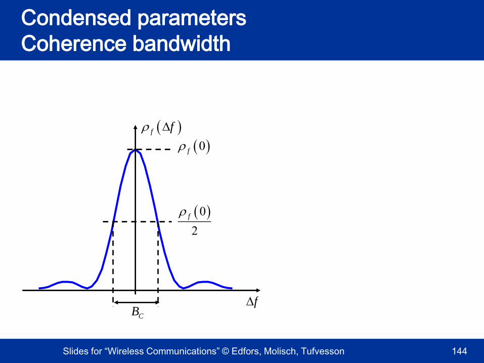
Defines the frequency difference that is required so that the frequency correlation coefficient is smaller than some threshold
Kenneth
Typewritten Text

145Slides for “Wireless Communications” © Edfors, Molisch, Tufvesson

Channel measures

Copyright: Shaker

146Slides for “Wireless Communications” © Edfors, Molisch, Tufvesson

Condensed parameters

The Doppler spectrum

Given the scattering function Ps (doppler spectrum as function of delay)

we can calculate a total Doppler spectrum of the channel as:

,B SP P d

For our tapped delay-line channel, we have:

2

2 2,max

2, iS i

i

P

2

2 2,max

2

2 21 ,max

2

2

iB i

i

Ni

ii

P d

Doppler spectrum of

tap i.

147Slides for “Wireless Communications” © Edfors, Molisch, Tufvesson

Condensed parameters

The Doppler spectrum (cont.)

We can “reduce” the Doppler spectrum into more compact descriptions

of the channel:

,B m BP P d

,

,

B

B m

B m

P dT

P

2

,,

B B m

B m

P dS T

P

2,

1

2N

B m i

i

P

, 0B mT

2 2,max

1

,

N

i i

iB

B m

v

SP

Total power (frequency integrated):

Average mean Doppler shift:

Average rms Doppler spread:

For our tapped-delay line

channel:

148Slides for “Wireless Communications” © Edfors, Molisch, Tufvesson

Channel measures

Copyright: Shaker

149Slides for “Wireless Communications” © Edfors, Molisch, Tufvesson

Condensed parameters

Coherence time

Given the time correlation of a channel, we can define the

coherence time TC:

t t

t

0t

02

t

CT

Kenneth
Typewritten Text
Kenneth
Typewritten Text
A measure of how fast a channel is changing Fast Fading - Coherence time is much less than symbol duration whereas slow fading is just the opposite. Fast fading only deals with the rate of change of the channel due to motion (user, IO's, etc.)

150Slides for “Wireless Communications” © Edfors, Molisch, Tufvesson

Condensed parameters

The time correlation

A property closely related to the Doppler spectrun is the time correlation

of the channel. It is in fact the inverse Fourier transform of the Doppler

spectrum:

exp 2t Bt P j t d

2

2 21 ,max

2

2 21 ,max

20 ,max

1

2 exp 2

2 exp 2

2 2

Ni

t

ii

Ni

ii

N

i i

i

t j t d

j t d

J t

For our tapped-delay line channel we get

Sum of time

correlations for

each tap.

151Slides for “Wireless Communications” © Edfors, Molisch, Tufvesson

It’s much more complicated than

what we have discussed!

Copyright: Shaker

152Slides for “Wireless Communications” © Edfors, Molisch, Tufvesson

Double directional impulse response

ht, r TX, r RX,,, 1

N r

ht, r TX, r RX,,,

TX position RX position

delay direction-of-departure

direction-of-arrival

ht, r TX, r RX,,, |a|e j

number of multipath components

for these positions

Kenneth
Typewritten Text
Kenneth
Typewritten Text
Kenneth
Typewritten Text
Kenneth
Typewritten Text
Kenneth
Typewritten Text
DDIR
Kenneth
Typewritten Text
Directional properties important for spatial diversity and multiple/directional antennas, e.g., MIMO and 802.11n
krgoodwin
Typewritten Text
The impact of the multipath components (MPCs) depends on the antennas used - changing antennas changes the impulse response
krgoodwin
Typewritten Text
krgoodwin
Typewritten Text
krgoodwin
Typewritten Text
krgoodwin
Typewritten Text
krgoodwin
Typewritten Text
krgoodwin
Typewritten Text
krgoodwin
Typewritten Text

153Slides for “Wireless Communications” © Edfors, Molisch, Tufvesson

Physical interpretation

l

Kenneth
Typewritten Text
TX
Kenneth
Typewritten Text
RX
Kenneth
Typewritten Text
Kenneth
Typewritten Text
Kenneth
Typewritten Text

154Slides for “Wireless Communications” © Edfors, Molisch, Tufvesson

Directional models

• The double directional delay power spectrum is sometimes factorized

w.r.t. DoD, DoA and delay.

• Often in reality there are groups of scatterers with similar DoD and DoA

– clusters

DDDPS,, APSBSAPSMSPDP

DDDPS,, k

PkcAPSk

c,BSAPSkc,MSPDPk

c

155Slides for “Wireless Communications” © Edfors, Molisch, Tufvesson

Angular spread

l

double directional delay power spectrum

angular delay power spectrum

angular power spectrum

power

Es,,,s,,, Ps,,,

DDDPS,, Ps,,,d

ADPS, DDDPS,,GMSd

APS APDS,d

P APSd

Matlab/Simulink - Communications System Toolbox