Chapter 6: Probability

I t d ti t P b bilitIntroduction to Probability

• The role of inferential statistics is to use th l d t th b i f the sample data as the basis for answering questions about the population.

• To accomplish this goal, inferential procedures are typically built around the concept of probability.

• Specifically, the relationships between samples and populations are usually samples and populations are usually defined in terms of probability.

P b bilit D fi itiProbability Definition

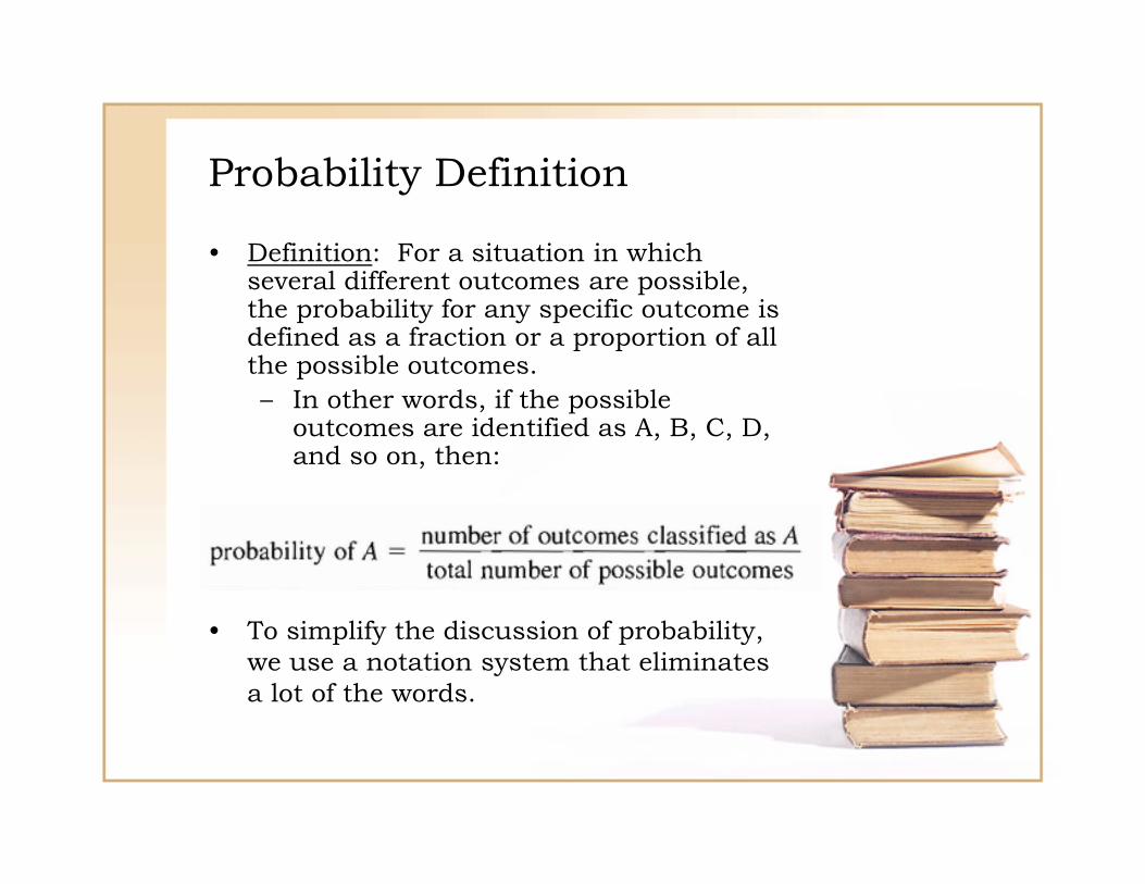
• Definition: For a situation in which l diff t t ibl several different outcomes are possible,

the probability for any specific outcome is defined as a fraction or a proportion of all the possible outcomes. – In other words, if the possible

outcomes are identified as A, B, C, D, and so on, then:

• To simplify the discussion of probability, we use a notation system that eliminates a lot of the words.

P b bilit D fi iti tProbability Definition cont.

• The probability of a specific outcome is expressed with a p (for probability) followed by the specific outcome in parentheses.

For example the probability of – For example, the probability of selecting a king from a deck of cards is written as p(king).

– The probability of obtaining heads for p y ga coin toss is written as p(heads).

• Note that probability is defined as a proportion, or a part of the whole. – In other words, this definition makes

it possible to restate any probability problem as a proportion problem.

P b bilit D fi iti tProbability Definition cont.

• By convention, probability values most often are expressed as decimal values.

• But you should realize that any of these three forms is acceptable.

F ti– Fraction– Proportion– Percentage

R d S liRandom Sampling• For the preceding definition of probability

to be accurate it is necessary that the to be accurate, it is necessary that the outcomes be obtained by a process called random sampling.

• Definition: A random sample requires that each individual in the population has an equal chance of being selected. – A second requirement, necessary for

many statistical formulas states that many statistical formulas, states that the probabilities must stay constant from one selection to the next if more than one individual is selected.

– To keep the probabilities from changing from one selection to the next, it is necessary to return each i di id l t th l ti b f individual to the population before you make the next selection.

R d S li tRandom Sampling cont.

– This process is called sampling with replacement.

• The second requirement for random samples (constant probability) demands that you probability) demands that you sample with replacement.

P b bilit d th N l Di t ib tiProbability and the Normal Distribution

• An example of a normal distribution is shown in Figure 6.3.

• Note that the normal distribution is symmetrical, with the highest frequency in the middle and frequencies tapering off in the middle and frequencies tapering off as you move toward either extreme.

• Although the exact shape for the normal distribution is defined by an equation (see y q (Figure 6.3), the normal shape can also be described by the proportions of area contained in each section of the distribution distribution.

• Statisticians often identify sections of a normal distribution by using z-scores.

Fig. 6-3, p. 170

Probability and the Normal yDistribution cont.• Figure 6.4 shows a normal distribution

with several sections marked in z-score units.

• You should recall that z-scores measure positions in a distribution in terms of positions in a distribution in terms of standard deviations from the mean.

• There are two additional points to be made about the distribution shown in Figure 6.4. – First, you should realize that the

sections on the left side of the di ib i h l h distribution have exactly the same areas as the corresponding sections on the right side because the normal distribution is symmetrical. y

Probability and the Normal yDistribution cont.

– Second, because the locations in the distribution are identified by z scores distribution are identified by z-scores, the percentages shown in the figure apply to any normal distribution regardless of the values for the mean and the standard deviation.

– Remember: When any distribution is transformed into z-scores, the mean b d th t d d becomes zero and the standard deviation becomes one.

• Because the normal distribution is a good model for many naturally occurring model for many naturally occurring distributions and because this shape is guaranteed in some circumstances (as you will see in Chapter 7), we will devote

id bl tt ti t thi ti l considerable attention to this particular distribution.

Fig. 6-4, p. 171

Probability and the Normal yDistribution cont.• The process of answering probability

questions about a normal distribution is introduced in the following example.

• Example 6.2 A th t th l ti f d lt – Assume that the population of adult heights forms a normal-shaped distribution with a mean of μ = 68 inches and a standard deviation of σ = 6 inches.

– Given this information about the population and the known proportions f l di ib i ( Fi for a normal distribution (see Figure 6.4), we can determine the probabilities associated with specific samples.

Probability and the Normal yDistribution cont.• For example, what is the probability of

randomly selecting an individual from this population who is taller than 6 feet 8 inches (X = 80 inches)?

• Restating this question in probability • Restating this question in probability notation, we get:

• We will follow a step-by-step process to find the answer to this question. – 1. First, the probability question is , p y q

translated into a proportion question: Out of all possible adult heights, what proportion is greater than 80 inches?

Probability and the Normal yDistribution cont.

– 2. The set of "all possible adult heights" is simply the population g p y p pdistribution.

– This population is shown in Figure 6.5(a).

– The mean is μ = 68, so the score X = 80 is to the right of the mean.

– Because we are interested in all h i ht t th 80 h d i heights greater than 80, we shade in the area to the right of 80. This area represents the proportion we are trying to determine. y g

– 3. Identify the exact position of X = 80 by computing a z-score. For this example,

Fig. 6-5, p. 172

Probability and the Normal yDistribution cont.• That is, a height of X = 80 inches is

exactly 2 standard deviations above the mean and corresponds to a z-score of z = +2.00 [see Figure 6.5(b)].

• 4 The proportion we are trying to • 4. The proportion we are trying to determine may now be expressed in terms of its z-score:

• According to the proportions shown in g p pFigure 6.4, all normal distributions, regardless of the values for μ and σ , will have 2.28% of the scores in the tail beyond z +2 00 beyond z = +2.00.

Probability and the Normal yDistribution cont.• Thus, for the population of adult heights,

Th U it N l T blThe Unit Normal Table

• To make full use of the unit normal table, there are a few facts to keep in mind: – The body always corresponds to the

larger part of the distribution whether it is on the right hand side or the leftit is on the right-hand side or the left-hand side.

• Similarly, the tail is always the smaller section whether it is on the right or the left.

– Because the normal distribution is symmetrical, the proportions on the i h h d id l h right-hand side are exactly the same

as the corresponding proportions on the left-hand side.

–

Th U it N l T bl tThe Unit Normal Table cont.

– Although the z-score values change signs (+ and -) from one side to the other, the proportions are always positive. Thus column C in the table always – Thus, column C in the table always lists the proportion in the tail whether it is the right-hand tail or the left-hand tail.

P b biliti P ti d SProbabilities, Proportions, and z-Scores

• The unit normal table lists relationships between z-score locations and proportions in a normal distribution.

• For any z-score location, you can use the table to look up the corresponding table to look up the corresponding proportions.

• Similarly, if you know the proportions, you can use the table to look up the y pspecific z-score location.

• Because we have defined probability as equivalent to proportion, you can also use h i l bl l k the unit normal table to look up

probabilities for normal distributions.

Probabilities, Proportions, and z-Scores , p ,cont.• In the preceding section, we used the unit

normal table to find probabilities and proportions corresponding to specific z-score values.

• In most situations however it will be • In most situations, however, it will be necessary to find probabilities for specific X values.

• Consider the following example: g p– It is known that IQ scores form a

normal distribution with μ = 100 and σ = 15.

– Given this information, what is the probability of randomly selecting an individual with an IQ score less than 130? 130?

Probabilities, Proportions, and z-Scores , p ,cont.• Specifically, what is the probability of

randomly selecting an individual with an IQ score less than 130?

(X 130) ?p(X < 130) = ?

• Restated in terms of proportions, we want to find the proportion of the IQ to find the proportion of the IQ distribution that corresponds to scores less than 130.

• The distribution is drawn in Figure 6.9, g ,and the portion we want has been shaded.

Probabilities, Proportions, and z-Scores , p ,cont.• The first step is to change the X values

into z-scores. – In particular, the score of X = 130 is

changed to

Th IQ f X 130 d • Thus, an IQ score of X = 130 corresponds to a z-score of z =+2.00, and IQ scores less than 130 correspond to z-scores less than 2.00.

• Next, look up the z-score value in the unit normal table.

Fig. 6-9, p. 178

Probabilities, Proportions, and z-Scores , p ,cont.• Because we want the proportion of the

distribution in the body to the left of X = y130 (see Figure 6.9), the answer will be found in column B.

• Consulting the table, we see that a z-score f 2 00 d t ti f of 2.00 corresponds to a proportion of

0.9772. • The probability of randomly selecting an

individual with an IQ less than 130 is individual with an IQ less than 130 is 0.9772:

• Finally, notice that we phrased this question in terms of a probability.

• Specifically, we asked, "What is the probability of selecting an individual with an IQ less than 130?"

Probabilities, Proportions, and z-Scores , p ,cont.• However, the same question can be

phrased in terms of a proportion: "What proportion of the individuals in the population have IQ scores less than 130?"

• Both versions ask exactly the same • Both versions ask exactly the same question and produce exactly the same answer.

Finding Proportions/Probabilities g p /Located Between Two Scores• The highway department conducted a

study measuring driving speeds on a local section of interstate highway.

• They found an average speed of μ. = 58 miles per hour with a standard deviation miles per hour with a standard deviation of σ = 10.

• The distribution was approximately normal.

• Given this information, what proportion of the cars are traveling between 55 and 65 miles per hour?

• Using probability notation, we can express the problem as

Fig. 6-10, p. 179

Finding Proportions/Probabilities g p /Located Between Two Scores cont.

• Looking again at Figure 6.10, we see that the proportion we are seeking can be di id d i t t ti (1) th l ft divided into two sections: (1) the area left of the mean, and (2) the area right of the mean.

• The first area is the proportion between The first area is the proportion between the mean and z = -0.30 and the second is the proportion between the mean and z = +0.70.

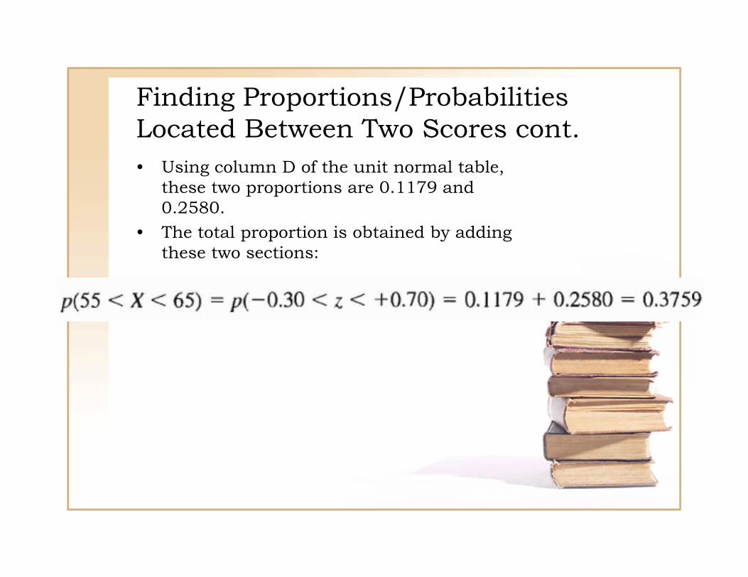
Finding Proportions/Probabilities g p /Located Between Two Scores cont.• Using column D of the unit normal table,

these two proportions are 0.1179 and 0.2580.

• The total proportion is obtained by adding these two sections:these two sections:

Finding Scores Corresponding to g p gSpecific Proportions or Probabilities• Scores on the SAT form a normal

distribution with μ = 500 and σ = 100. • What is the minimum score necessary to

be in the top 15% of the SAT distribution? (An alternative form of the same question (An alternative form of the same question is presented in Box 6.2.)

• This problem is shown graphically in Figure 6.13. g

• In this problem, we begin with a proportion (15% = 0.15), and we are looking for a score.

• According to the map in Figure 6.12, we can move from p (proportion) to X (score) via z-scores.

Finding Scores Corresponding to Specific g p g pProportions or Probabilities cont.• The first step is to use the unit normal table

to find the z-score that corresponds to a proportion of 0.15.

• Because the proportion is located beyond z in the tail of the distribution we will look in the tail of the distribution, we will look in column C for a proportion of 0.1500. – Note that you may not find 0.1500

exactly, but locate the closest value y,possible.

– In this case, the closest value in the table is 0.1492, and the z-score that

d hi i i 1 04 corresponds to this proportion is z = 1.04. • The next step is to determine whether the z-

score is positive or negative. • Remember that the table does not specify the • Remember that the table does not specify the

sign of the z-score.

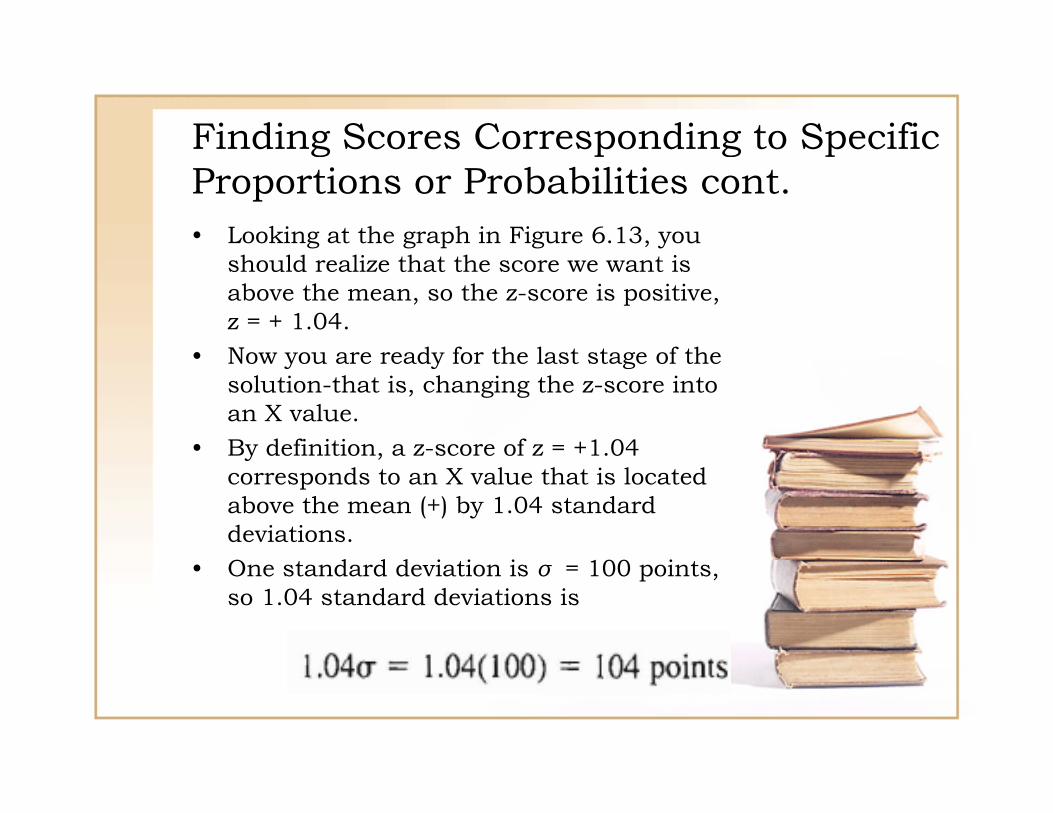
Finding Scores Corresponding to Specific g p g pProportions or Probabilities cont.• Looking at the graph in Figure 6.13, you

should realize that the score we want is above the mean, so the z-score is positive, z = + 1.04.

• Now you are ready for the last stage of the • Now you are ready for the last stage of the solution-that is, changing the z-score into an X value.

• By definition, a z-score of z = +1.04 y ,corresponds to an X value that is located above the mean (+) by 1.04 standard deviations. O d d d i i i 100 i • One standard deviation is σ = 100 points, so 1.04 standard deviations is

Finding Scores Corresponding to Specific g p g pProportions or Probabilities cont.• Thus, our score is located 104 points

above the mean. • With a mean of μ = 500, the score is X =

500 + 104 = 604. Th l i f thi l i th t • The conclusion for this example is that you must have an SAT score of at least 604 to be in the top 15% of the distribution.

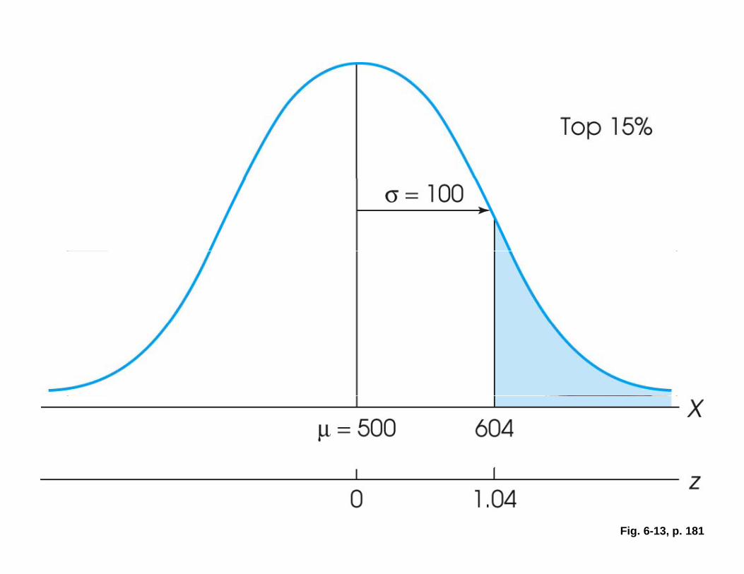
Fig. 6-13, p. 181