Chapter 6: Market equilibrium (1.1)

If it’s not part of the solution…

…then it’s part of the problem. The simple function of a market is to put both parties – customers and suppliers – in touch with

other. The rest follows: any given want of a potential buyer will result in search behaviour, and the opportunity costs of that

search are lowest where a great many items may be seen and compared in the shortest amount of time. The lower opportunity

cost is thus; the potential buyer can compare a great many similar goods in short order and perhaps bargain the way towards the

highest satisfaction. This is far more efficient than gallivanting around the countryside in search of 20 different items. Th e

market is simply a very efficient method of displaying the merchandise.

The same holds for providers of goods, as the demand is a signal to suppliers as to what goods should be provided and what th e

going price is. If the price is attractive and/or the demand is high then rest assured that the supplier will be back the next time

with more goods for sale! Should there be too many similar goods for sale, then one can assume that a number of suppliers will

put effort into finding other or better goods to sell – or other places to sell them. If the going market price is too low for a

supplier to be able to sell his/her wares, then there is a strong incentive for the supplier to increase efficiency in order to lower

costs – and thus compete on the market.

The market thus functions as a mechanism to fulfil both customers ’ and suppliers’ wants. The market system also addresses the

issue of excess and quality; any superfluous goods are simply not sold at the existing price. Market dynamics have thus solve d

the basic economic problem of what, how and for whom: consumers ’ demand decides what is to be produced; basic

competition between suppliers addresses the issue of how to produce (as inefficient producers are forced to leave the market) ;

and the price decides who gets the goods.

Key concepts:

Excess demand and excess supply

Equilibrium (market clearing)

Change in demand (e.g. shift of demand curve) change in quantity

supplied (e.g. a movement along the supply curve) o Tastes/preferences, price of substitutes, price of complements,

advertising…

Change in supply (e.g. shift of supply curve) change in quantity

demanded (e.g. a movement along the demand curve) o Market factors

o Scarcity of factors of production o Quality/quantity of factors of production o Non-market variables, i.e. intervention

HL extensions:

Equilibrium price and quantity – linear supply and demand functions

Plotting linear supply and demand curves to identify equilibrium price

and quantity o Excess demand/supply in diagrams

As long as we are all good comparison shoppers and firms operate from within competitive forces, the system will provide the

‘right amount of goods ’ at the ‘correct price’. In theory, that is. Unfortunately, as we shall see, for the tooth fairy to deliver, one

has to knock out a few teeth.

Excess demand, excess supply and equilibrium “I am like any other man. All I do is supply a demand.” - Al Capone

In class, I often bring up the open markets I’ve visited. I describe them in some detail in terms of the time spent putting shoddy goods out for sale. I still claim that many of them obey only half the law of supply/demand; if something ‘sucks’ there’s always plenty of it. I have more or less observed this in virtually every country I’ve been to. My conclusion; too many people have too much free time on their hands.

In any case, market clearing – e.g. market equilibrium – is at the heart of the concept of market dynamics, which is based on

how the interaction of supply and demand creates a market price. Let us continue with the market for DVD films.

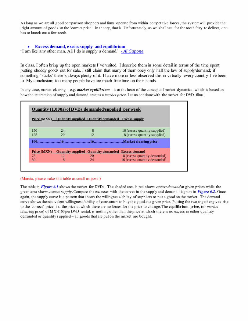
(Marcia, please make this table as small as poss.)

The table in Figure 6.1 shows the market for DVDs. The shaded area in red shows excess demand at given prices while the

green area shows excess supply. Compare the excesses with the curves in the supply and demand diagram in Figure 6.2. Once

again, the supply curve is a pattern that shows the willingness/ability of suppliers to put a good on the market. The demand

curve shows the equivalent willingness/ability of consumers to buy the good at a given price. Putting the two together gives rise

to the ‘correct’ price, i.e. the price at which there are no forces for the price to change. The equilibrium price, (or market

clearing price) of MXN100 per DVD rental, is nothing other than the price at which there is no excess in either quantity

demanded or quantity supplied – all goods that are put on the market are bought.

Price (MXN) Quantity supplied Quantity demanded Excess demand

75 12 20 8 (excess quantity demanded) 50 8 24 16 (excess quantity demanded)

100……………….16 …………………16……………………Market clearing price!

150 24 8 16 (excess quantity supplied)

125 20 12 8 (excess quantity supplied)

Quantity (1,000s) of DVDs demanded/supplied per week

Price (MXN) Quantity supplied Quantity demanded Excess supply

Figure 6.1: Excess supply/demand and market clearing for DVDs

Figure 6.2 shows how at any price above MXN100 suppliers have an incentive to put too much on the market. The high price

acts as a signal to suppliers to put more of the good on the market. However, consumer demand at prices above MXN100 is less

than the amount suppliers would put on the market, there is excess supply (or surplus). Firms supplying DVDs will soon

discover that they are stocking too many DVD films and will act to cut this amount. This market glut will therefore cause a

downward movement in price as suppliers begin to lower prices and cut excess films on their shelves. (It is worthy of revising

the concept of opportunity cost here. Just imagine how costly it is for a supplier of DVD films to have purchased 50 copies of

Paris Hilton’s latest epic drama only to discover that 49 of them sit on the shelf week after week.1 The shelf space could be

used for other items – other DVD films or complement goods such as potato chips – and the supplier’s cost of obtaining the

films means that these resources could have been put to better use.)

In the same manner, if the price is set belowMXN100, consumers will demand more DVDs than will be supplied during the

week. This excess demand will mean that suppliers have empty shelves and full queues of customers. The price is evidently too

low so they will raise the price. This will act as a stimulus and incentive for supp liers to re-stock the shelves quicker in answer

to the excess demand. More DVD films will be made available. An increasing market and the resulting increase in quantity

supplied means that the excess demand will decrease as price moves towards equilibrium at MXN100 per DVD.

The above illustrates the price mechanism at work. Another way of looking at the dynamics of supply, demand and price is that

suppliers will want to charge as much as possible and consumers will want to pay as little as possible. It is in this arena that the

bargaining process will play out. I often find it useful to think of the supply and demand interplay as a form of auction. Th ere

are a given number of goods at an offered price and it is now up to consumers ’ demand to arrive at a price whereby the

proffered goods are sold. Highly demanded goods will be ‘bid up ’ in price while unsold goods will be ‘auctioned off’ at lower

prices.

1 I wonder if the stretch of prison time for poor Paris increased demand for her DVDs. Marketing gimmick?

S

Q/t (1,000s DVDs/week)

P (MXN/DVD)

8 16 24

D

50

150

100

Excess demand of 16,000

DVDs/week at a price of

MXN50; prices will be forced

upwards.

Excess supply of 16,000

DVDs/week at a price of

MXN150; prices will be

forced downwards.

No excess demand or excess

supply = market clears

********************************************************************

POP QUIZ 6.1 MARKET EQUILIBRIUM

1. Below are some figures for the supply of wheat during a three month period. What is the equilibrium price per tonne?

(Qd = quantity demanded, Qs = quantity supplied, P = price)

P ($) Qs (tonnes) Qd (tonnes)

3 2 20

4 4 16

5 6 12

6 8 8

7 10 4

8 12 0

2. What would be a possible effect on the market in question one above if the quantity demanded was higher than the

quantity supplied and the price was fixed by law?

*********************************************************************

Change in demand The Saga (= story) continues. Recall that our so-called equilibrium price is in actual fact the price at which the market clears

within a given period of time. What if a non-price determinant of demand were to change within the given time frame? The

main non-price determinants of demand are income, price of substitutes/complements, tastes/preferences and changes in

population composition.

For example, what if Swedish consumers ’ preferences changed in favour of more environmentally friendly modes of

transportation – for example bicycles? This would shift the demand curve for bicycles from D0 to D1, as shown in Figure 6.2.

At the new level of demand, there would be more willing buyers than supply on the market (e.g. excess demand) at P0 and this

would force prices upwards from P0 to P1 causing suppliers to increase the quantity supplied (Q0 to Q1). This is the same as

saying that the increase in demand (= shift of demand curve) has caused upward pressure on the (equilibrium) price and an

increase in quantity supplied. In economics we write this as “…the increase in demand (D0 to D1) causes an excess in demand

Story time! I simply have to tell the story of my old man’s (= father’s) experience at an open market in Mexico City in

the mid-1960’s. An old lady had a large blanket spread out on the zócalo (= main plaza or square) with a

largish pile of limes on it. My father, of course, needed limes for the evening cocktail party with the

expatriate crowd. He asked “how much” and got a price quote per kilo and then asked “How much for the

entire pile?” expecting a better deal. The old lady doubled the price! My utterly confused old man

stammered out a question as to why the price was higher since he was prepared to buy them all. The answer;

“Ah, señor. If I sell you all my limes I will have nothing to do for the rest of the day and I will go home.

Then I won’t be able to see all my friends here at the zócalo.” I love the answer, for two reasons. One, it

shows the limits of “market clearing theory”, and two, there are people for whom there are things more

important than profit. There’s hope. *** We had this in a “Story time” with a neat market picture.***

at the original price and therefore upward pressure on the price (P0 to P1) and an increase in quantity supplied (Q0 to Q1)…”2

In economic shorthand: ↑Dbicycles → QD>QS at P0 → ↑Pbicycles → ↑QS QS = QD at P1

This is perhaps the most important conclusion so far within our market model: a change in demand is price-determining –

while a change in quantity demanded is price-determined! When demand for bicycles changes – for example, due to a change

in preferences for cycling – then the entire demand curve will shift, causing the price to change and a movement along the

supply curve.

Figure 6.2: Increase in demand for bicycles

Naturally, there are a goodly many other non-price variables that would cause demand for bicycles to increase as in figure 6.2

but rather than spell them out for you I’ve inserted a…

*******************************************************

…POP QUIZ 2.1.4 NON-PRICE VARIABLES AND DEMAND

1. How would demand for bicycles (in figure 6.2 above) be affected if the price of gasoline fell?

2. What other variables could affect demand as illustrated above in figure 6.2?

**************************************************

2 This is an important lesson in what economists call causality, i.e. the forces of cause and effect. The change in demand causes a change in

price – which in turn causes and increase in quantity supplied.

P0

P1

P(SEK/bicycle)

S

D1

Excess quantity demanded at P0

D1

Q0

Q1

Q2

Q/t

(bicycles/month)

A

B

C D

An increase in

demand (D0 to D1)…

…causes excess

demand at P0 (Q0 ↔

Q2)…

…which forces up

the market price (P0

to P1)…

…leading

suppliers to increase

quantity supplied (Q0

to Q1).

A

B

C

D

The world’s f irst proper stock market was f ounded in the early 17th century in

Amsterdam. It didn’t take too long bef ore there was rash speculation, a commodity

boom and ensuing crash – all within the time-f rame of less than f our y ears.

Tulips arriv ed in Holland in the mid 16th century

f rom Eastern Mediterranean countries, where they

grew in the wild, most likely f rom Turkey . They were

greatly appreciated and horticulturists set about

breeding many new v arieties of tulips. Many of

these new ty pes were rare and thus most cov eted

by the rich of Holland. They became sy mbols of

status and sophistication in the upper class.

It didn’t take long bef ore enterprising merchants,

dock workers, captains of ships, f armers and citizens f rom ev ery walk of lif e started

to speculate in an endless ascension of the v alue of tulips. Tulip speculation was

based on the selling of bulbs (by weight). They came to be sold, speculated and

used as collateral f or loans. Also, due to being highly seasonal, much of this was

while the tulip bulbs were still in the ground – and nobody had actually seen the

f lowers as y et! Talk about a bubble – this trade actually was ref erred to as‘wind

trade’.

Rare bulbs f etched preposterous prices as speculativ e euphoria and mass psy chosis

reached its pinnacle in 1636/37; a bulb of theSemper Augustus ty pe worth 1,000

guilders in 1623 was sold f or 5,500 guilders in 1637 – more than USD55,000 at

today’s prices. Traders in tulips could earn 5,000 guilders in a month where the

av erage income at the time was 150.

This mania came to a screeching halt during 1637 when some of the more cautious

and perhaps f oreseeing speculators started to leav e the market by selling of f their

stock without replenishing it. A chain reaction set of f where f alling prices ultimately

saw ev ery one try ing to sell their stock bef ore prices f ell ev en f urther. The bottom f ell

out of the market and prices went down to under 10% of peak market v alues. A great

many f ormerly wealthy people lost their f ortunes to speculation as they stood af ter

the crash with enormous debt and only tulip bulbs – now deemed worthless – as

security f or this debt.

Sources: Dash, M.,Tulipomania : The Story of the World's Most Coveted Flower &

The Extraordinary Passions it Aroused. Crown Publ., 1999. Also: Galbraith, John

Kenneth; A short history of financial euphoria, 1993, Penguin Books.

STORY FROM HISTORY:

TULIPMANIA IN 1637

Change in supply Let us look at how a change in supply results in a change in price and thus quantity demanded. In Figure 6.3 we can see how

an increase in the supply of coffee, say due to a bountiful harvest of coffee beans (which is a factor input in the production of

coffee), shifts the supply curve for coffee to the right. This is intuitively self-explanatory; an increase in market supply will

create relative abundance of the good (within the time period in question) and an excess supply of coffee at the initial price P0

and thus force the price downwards towards the new equilibrium (at P1). The increase in supply (S0 to S1) has caused the

equilibrium price to fall (P0 to P1), in turn leading to an increase in quantity demanded (Q0 to Q1).

In economic shorthand: ↑Scoffee→ QS>QD at P0 → ↓Pcoffee → ↑QD QS = QD at P1

Figure 6.3: Market for coffee – increase in supply

In a similar vein, anyone who has experienced abnormally bad weather during the growing season for any number of

vegetables and fruits can instinctively predict how the price of coffee would be forced upwards due to detrimental growing

conditions and the ensuing hit to supply of green coffee. Other non-price variables which would cause the supply of coffee to

increase are:

o Scarcity/abundance of factors of production – increased land available for coffee growing o Price of factors of production – a fall in the price of farm implements or electricity o Technology (“quality of factors”) in production – better coffee strains which yield more crops o Expectations of producers – if coffee growers expect a surge in demand in the future

************************************************************

POP QUIZ 6.2 EFFECTS OF NON-PRICE VARIABLES ON SUPPLY

1. How might the increase in supply of coffee shown in figure 6.3 above affect the market for cocoa?

2. How might cocoa producers act if they knew in advance that the supply of coffee was going to increase?

************************************************************

We’re cooking now, right? So, how hard can it be to make a logical jump over to the outcome of a decrease in supply or

demand? This is shown in Figures 6.4a and b. In a, we see how supply for a good has decreased from S’0 to S’1 (for example

due to increasing labour costs), and how the price has adjusted upwards from P’0 to P’1 and quantity demanded has

consequently decreased from Q’0 to Q’1. In b, demand has decreased from D0 to D1 (say due to a fall in the price of a substitute)

forcing the equilibrium price downwards from P0 to P1, decreasing quantity supplied from Q0 to Q1 .

In economic shorthand (fig a): ↓S’→ ↑P’ → ↓Q’D Q’S = Q’D at P’1

In economic shorthand (fig b): ↓D → ↓P → ↓QS QS = QD at P1

Figure 6.4a) and b) : Decrease in supply and decrease in demand

An increase in

supply (S 0 to S 1)…

Q/t (kgs/season)

…causes excess

supply at P0 (Q0 ↔

Q2)…

…and this forces

down the market

price (P0 to P1)…

…leading to an

increase in quantity

demanded (Q0 to Q1).

P0

P1

P(USD/kg)

S0 D

Excess quantity supplied at P0

Q0

Q1

Q2

A

A

B

C

D

S1

D

B

C

Large Matt-heading: Supply and demand analysis

My father had firm views on child rearing.3 Basically, his methodology might be termed ‘Darwinistic Nurturing’ – or, today,

“child abuse”. Learning how to swim was on a ‘sink-or-swim’ basis, where I got the basic techniques in the Sheraton Hotel

pool and gained hard-earned experience by getting tossed into the sea from the boat. ‘We’ll pull ashore on the little island over

there, Matthew. Keep your chin up.’ This, incidentally, in the Caribbean Sea where one could be accompanied at any time by

barracudas, sharks, highly poisonous jellyfish – and where the seabed was littered with sea urchins s porting six inch spikes. A

3 “Don’t have any!”

One of the most common errors of my fresh students is in insisting on shifting the supply

curve in order to show how suppliers react to changes in demand – the explanation being

that “…the increase in demand causes an increase in supply…”

The second common error is in insisting on shifting the demand curve to show how

consumers react to a shift in supply, e.g. “…the increase in supply causes an increase in

demand…”

Both are technically erroneous, absolutely superfluous and just plain wrong!

Any shift of the demand curve already SHOWS how suppliers will react (e.g. a change in

supplied quantity) without any further assistance from the supply curve. In a similar mode,

shifting the supply curve shows how consumers will react (change in quantity demanded)

and no shift in the demand curve is necessary.

P0

P1

P ($/unit)

Q0

Q1

Q/t

S

D0

D1

P’0

P’1

P’($/unit)

S’1

D

Q’0

Q’1

Q’/t

S’0

A decrease in supply (S’0 to S’1)

forces the price up (P’0 to P’1) and

thus causes a decrease in the quantity

demanded (Q’0 to Q’1)

A decrease in demand (D0 to D1)

forces the price down (P0 to P1) and

thus causes a decrease in the quantity

supplied (Q0 to Q1)

a) Decrease in supply

b) Decrease in demand

WARNING! Increase in demand ≠ increase in supply

few added flotation incentives, you might say.

And that is how a good deal of your own applications of economics will be played out in the remaining examples . It is

impossible to give extensive examples of the virtually endless uses of the supply and demand model – you will mostly learn by

doing. However, I conclude this chapter with two basic examples of market interaction, using the basic tools of supply and

demand and linking to previous concepts. Then I leave it to you to learn how to re-apply economic illustrations to whatever

real-life scenarios you need to deal with in exams or internal assessment. Sink or swim people.

Matt-heading under large heading above: Supply and demand (plus reallocation) analysis number one: ‘Oh

lord, won’t you buy me a Mercedes Benz?’4

One of my IB1 kids’, Nico’s, (Marcia; where do the apostrophes go?!) father is one of the largest retailers of cars in Mexico –

something he no doubt regrets since I’ve had him put me on the short list of “Favoured Customer” for a new 425 horse power

Dodge Charger.5 I started looking for the Charger with my pal Toni last year, who basically has said “Mateo, for crying on a

crutch; just get it! You can afford it…give up a new wristwatch or two.” I patiently explained that I was waiting for prices to

fall like a paralysed parakeet; “Toni, by the time I’m ready to buy, Nico’s dad is going to pay me to get it off the parking lot

and have two of the cute salesgirls go with me!” Am I as crazy as my colleagues say I am? We ll, not in economics at least – let

me explain. (Need a pic of a Dodge Charger here.)

The high cost of gasoline (during what will probably become known as the “Speculative oil crisis of 2008”) is changing

consumers’ behaviour. Gasoline and cars are very close complements. As the price of gasoline surged during 2007 and 2008,

households increasingly switched from large to small “Econo -cars”, i.e. demand decreased considerably for large gas -guzzling

cars, shown in Figure 6.5a (D0 to D1).This was associated with an increase in demand for available substitutes, in this case

more fuel-efficient cars. This is shown by the increase in demand from D’0 to D’1 for fuel-efficient cars in Figure 6.5b.

4 This is the title of an absolutely incredible song by Janis Joplin. 5 For reasons unknown to me, my students at some point always want to know what type of car I drive and invariably expect the answer to

be either a Mercedes or a BMW. I assume it’s because I wear a suit and tie but they’ll probably give ‘machismo’ as their answer. There might

be something in it. In sensible Sweden I drove very sensible cars; VW Polos and Toyota Corollas. Here in Mexico I went for sp eed, power

and mass – an Audi A6 Turbo with 250 HP. Anything to intimidate, escape from and/or turn into purée the robo-cops (play on words; “robo”

is “robbery” in Spanish) and wild dogs – both of which clutter up the highways when I’m enjoying complement goods. Life expectancy; T

plus 2 years and counting.

Figure 6.5: Car market – reallocation of resources

Now, I know what you’re thinking. Didn’t I – in both figure 6.5a) and b) – just break the rule of ‘…not shifting supply due to a

shift in demand…’?! No – because there’s more to the above story. You see, automobile manufacturers were preparing for the

surge in demand by taking factors of production no longer needed in Gas -guzzlers and putting them to work in the Econo-car

production plants. Resources were being reallocated to the production of fuel efficient cars in order to increase output during

the on-going ‘switch-over period’. This is shown in figure a) by the decrease in supply of gas-guzzling SUVs (S0 to S1)

resulting in a further decrease in the quantity of SUVs purchased on the market (Q2) and an equilibrium price of P2. In figure

b), the increase in supply from S’0 to S’1 for Econo-cars was the result of resources being reallocated to small fuel efficient cars.

I have shown – rather speculatively, it should be noted – how the equilibrium price for Gas-guzzlers goes down due to the

P0

P2

P (MXN/car)

Q0

Q2

Q/t (cars/month)

S0

D0

D1

P’0

P’1

P’(MXN/car) S’1

D’0

Q’0

Q’1

Q/t (cars/month)

S’0

a) Gas-guzzlers (SUVs)

b) “Econo-cars”

D’1

A

B

C

P’2

Q’2

S1

P1

Q1

Fig. a) As the price of

gasoline rises, the demand for

large fuel inefficient cars decreases (D0 to D1) leading to

a fall in price (P0 to P1) and a

decrease in quantity demanded

(Q0 to Q1).

A

Fig. b) As consumers shift

towards “Econo-cars”, demand

increases from D’0 to D’1 leading to upward pressure in

price (P’0 to P’1) and an

increase in quantity supplied

(Q’0 to Q’1).

B

Fig. a) As suppliers

anticipate continued decreases

in demand for Gas-guzzlers, they start to scale back

production (S 0 to S 1 )…

Fig. b) …and reallocate

resources to “Econo-car” production, shown by the

increase in supply from S’0 to

S’1. Equilibrium settles at P’2

and Q’2.

C

C

decrease in demand for them outstripping (= exceeding) the decrease in supply.6 Equally speculatively, the price of Econo-cars

increases since the increase in demand outstrips the increase in supply.

Basically what oil and gasoline prices are doing are reallocating resources via the laws of supply and demand. There is an

enormous incentive for car makers to divert resources from high fuel-consuming cars to more efficient cars. This is an example

of the process of reallocation.

Supply and demand analysis number two. “Tortillas and oil” "While many worry about filling their gas tanks, many others around the world are struggling to fill their stomachs. And it's

getting more and more difficult every day." World Bank President, Robert Zoellick, (The Guardian, 30 April 2008)

*** Pic; Marcia’s “Protesters in Mexico City demonstrate…”

It was applied economics in the making; we watched, week by week, how oil prices wreaked havoc (= chaos) on poor families

in Mexico. No, not because of rising gasoline prices – gasoline is heavily subsidised in Mexico – but because of ever higher

prices for maize and maize tortillas. World food prices – according to the International Monetary Fund (IMF) – rose by some

45% between the end of 2006 and April 2008. In Mexico, for the 50% of the country’s 106 million citizens living on less than

five US dollars a day, the staple (= basic, essential) food is the tortilla – a flat “pancake” like bread made of maize meal (corn

flour). When the price of maize skyrocketed during 2007/’08 the effect was to cause the price of tortillas to increase from

around 7 Mexican pesos (MXN) to over MXN10.7 I didn’t notice the price increase – but I don’t live on USD5 a day as

millions of Mexicans do.8 I did, however, notice the thousands of protesters in Mexico City banging empty pots against the

walls of government buildings.

So what caused the rise in the price of tortillas? A number of things – all related. The main cause was the surge in oil and

gasoline prices which caused a somewhat frantic search for substitutes. One of these substitutes is ethanol (alcohol) made from,

primarily, sugar and maize. US farmers started shifting agricultural land (standard example of reallocation of resources!)

6 Several of my students have gleefully pointed out that the Mexican police are in the process of changing all their old cars for new Chargers

– which in fact might increase the price of this particular model. Our bribe…em, tax money in action. 7 The exchange rate then was between MXN10.5 to MXN11 for 1USD. 8 The official minimum wage in Mexico (at the current exchange rate of USD1 = MXN13.5) is just over USD4. It rather makes sense why my

Mexican ex-lady friend refused to get in the car with me if I was wearing one of my watches. Basically, my Rolex GMT Master II represents

about 6 years minimum wage and she didn’t want to be a collateral victim of highway robbers due to my nonchalant habit of let ting my left

arm hang out the car window during traffic. Affectionate parents who invite me to parties inevitably send a car and driver for me since I

refuse to wear a cheapo watch. Maybe they figure I need both hands to do term reports.

Internal Assessment tip At this stage of your studies in economics you should be able to use basic concepts and diagrams in your Internal

Assessment (IA) commentaries. I urge you to spend some time searching for appropriate articles and not simply

cut something out the day before your deadline! Getting hold of a good article is half the battle.

1) Avoid articles where the analysis is already done for you. You get no points for simple re-iteration of

someone else’s analysis.

2) Don’t pick overly complicated issues – there’s nothing wrong with applying your acumen (= insight)

and economic knowledge to day-to-day issues, such as why the municipality wishes to make public

swimming pools available by lowering price of admission.

3) It is generally more fruitful to chose a relatively brief article (not too brief!) and build up a structure of

economic arguments, rather than to choose a long article and comment generally on a few definitional

points. Do NOT use the small “notices” that newspapers often put in the margins. Use proper articles.

4) Diagrams are to be used to support the iteration – not replace it! Make sure that your diagrams are neat,

numbered and well referred to in the text and not simply left hanging. This makes it easier for your

teacher to follow your thread of thought.

Don’t waste time going through stacks of newspapers/journals but be smart. Do a “Google” and simply type in a

search string containing key words which might be dealt with via your knowledge of economics at this stage. For

example, during 2007/’08 I suggested my people try “…gasoline + oil + demand + supply + tortillas + maize +

solar power + wind power + silicon…”. Wonder what I’m on about?! Read the next section on “Tortillas and

oil”.

towards the production of maize and increasingly sold this for use in ethanol production. Hence, as maize meal for tortillas and

maize for ethanol are in joint supply, an increase in demand for ethanol in the US served to decrease the available supply of

maize for foodstuffs . How could this affect Mexico which supplies most of the maize for its domestic market? Three causes

stand out: competition laws, higher import prices and speculation – but not necessarily in that order of occurrence or

importance. Let me do a brief point-by-point explanation:

1. Mexico has allowed imports of maize since 19949 but has limited these imports to protect domestic farmers from the

very efficient and heavily subsidised American farms. However, 80% of imported maize in Mexico comes from the

US. As fuel prices in the US soared and ethanol demand subsequently increased (recall that an increase in the price of

a good will increase demand for substitutes) more and more US maize was diverted towards ethanol, creating a surge

in maize prices.

2. This decreased the US supply of maize for exports and increased the price of imported maize to Mexico.

3. The main maize suppliers for tortillas in Mexico are, somewhat notoriously, operating in an oligopoly market. There is

ample evidence that domestic Mexican suppliers withheld maize in speculative anticipation of higher future prices.

The causal flows (oil maize tortillas) are illustrated in figure 2.1.31a, b and c.

Demand for oil increased (figure a) during 2006 – 2008 due to increasing demand from oil hungry countries –

primarily India and China – and speculation of higher prices. While suppliers attempted to increase production of oil,

demand far outstripped supply. This caused gasoline prices to double in the US during the time period and

consequently caused a search for substitutes – primarily ethanol.

This in turn caused an increase in demand for maize to produce ethanol. It also caused maize growers to step up maize

production to meet ethanol demand. This is illustrated in figure b by the increase in demand from D’0 to D’1 and the

increase in supply from S’0 to S’1. Since more US maize was now going to the production of ethanol, the available

supply of maize for the Mexican market decreased and Mexican import prices for maize shot up.

This resulted in higher production costs for Mexican tortilla producers, shown by decrease in supply (S*0 to S*1) in figure c. When maize producers in Mexico acted upon expectations of higher world market prices for maize, they

started to hoard supplies, e.g. they held off on releasing enough maize to meet current demand in speculation of higher

future prices.

The decrease in maize flower (factor input in tortillas) further increased production costs for tortilla producers,

decreasing supply (S*1 to S*2) and drove up the price of tortillas by some 200% during the first months of 2007.10

(Rory: still issues with my tenses.)

9 When the North American Free Trade Agreement came into effect. 10 See http://www.nytimes.com/2007/01/19/world/americas/19tortillas.html, http://www.reuters.com/article/GCA-

Agflation/idUSN1451427920080514 and http://news.bbc.co.uk/2/hi/americas/7432164.stm

Figure 6.5: Oil, maize and tortillas in Mexico, 2006 – 2008

P1

P (USD/barrel)

Q/t (barrels/month)

S0

D0

D1

a) Oil (global)

S1

P0

Q0 Q1

As global demand for oil

drastically outstripped supply

during 2006 – 2008, the price of

oil and thus gasoline in the US

rose.

A

The search for available

substitutes – here, ethanol –

caused an increase in demand

for maize (D’0 to D’1), in excess

of the increased supply (S’0 to S’1), causing an increase in the

price of maize (P’0 to P’1).

B

As more US maize was

diverted towards ethanol

production, available imports to

Mexico of maize from the US

decrease which in turn increased costs for tortilla

producers. The supply of

tortillas decreased

(S*0 to S*1 )…

…and at the same time,

speculative forces in Mexico

lead to hording of maize

amongst maize suppliers raising

maize prices further, and a further decrease in the supply of

tortillas (S*1 to S*2.) Tortilla

prices had trebled by January

2007 (P*2).

C

A

P’1

P (USD/tonne)

Q’1

Q/t (tonnes/month)

S’0

D’0

D’1

S’1

P’0

Q’0

b) Maize for ethanol (US)

B

P*2

P (MXN/kg)

Q*1

Q/t (kgs/month)

S*0

S*2

S*1

P*0

Q*0

c) Tortillas (Mexico)

C

D*

P*1

Here it was my intention to continue with the secondary and tertiary effects on the markets for solar power, silicon and

computers. But I’m tired, so I shall instead turn to the trusted method of didactic (= educational) laziness etched in stone tablets

by countless generations of teachers since the days of Ivied Castles all around, hi-ho. Yes, you guessed it; I will pose more

questions.

POP QUIZ 2.1.7 SUPPLY AND DEMAND

1. Re “Tortillas and oil” above: How might the price of oil have affected the price of solar panels in the US?

2. Re “Tortillas and oil” above: How might the price of oil have affected the price of silicon? (This is a continuation of

Question 1 above. Hint; look up “photovoltaic cells” and “silicates”.)

3. Re “Tortillas and oil” above: How might the price of oil have affected the supp ly of computers? (This is a continuation of

Question 2 above. Did you look things up?)

4. ‘In some countries the price of houses rises while the demand for houses rises ’. Using supply and demand analysis, explain

why this statement does not contradict the law of demand.

5. Using supply and demand diagrams, explain how the price of seasonal goods would be prone to fluctuate during a year. ´

6. You believe that property prices will soon plummet (= fall drastically). Being a property -speculator, you act on this belief.

Illustrate the possible outcome of this situation using supply and demand curves. Assume that other speculators will follow

your lead.

HL extensions

Equilibrium price and quantity – linear supply and demand functions and calculating equilibrium

price and quantity Now we put the two functions together and calculate equilibrium. Keep in mind that:

a) If Qd = Qs, then the demand function yields the same values – price and quantity – as the supply function

b) Thus, in equilibrium; a – bP = c + dP

Qd = a – bP and Qs = c + dP

Assume the following demand and supply functions: Qd = 4,000 – 20P and Qs = -2,000 + 40P

Putting this into a table shows that market equilibrium is established at a price of $100 and quantity of 2,000 units.

P Qd ($) Calculation P Qs ($) Calculation

0 4,000 Qd = 4,000-20*0; 4,000 0 -2,000 Qs = -2,000 + 40 * 0; -2000

50 3,000 Qd = 4,000-20*50; 3,000 50 0 Qs = -2,000 + 40 * 50; 0

100 2,000 Qd = 4,000-20*100; 2,000 100 2,000 Qs = -2,000 + 40 * 100; 2,000

150 1,000 Qd = 4,000-20*150; 1,000 150 4,000 Qs = -2,000 + 40 * 150; 4,000

200 0 Qd = 4,000-20*200; 0 200 6,000 Qs = -2,000 + 40 * 200; 6,000

Basically finding market equilibrium is a matter of solving one unknown, for example P. Thus solving the following equation

(“simultaneous equation” in math speak) will find P:

Assuming market equilibrium, where Qd = Qs, we equate the equations to get 4000 - 20P = -2000 + 40P11

o 6000 = 60P; P = 6000/60; P = 100

Now we solve for Qd or Qs by simply substituting P = 100 in either function:

o Qd = 4000 – 20 x 100; 2,000 units

o Qs = -2000 + 40 x 100; 2,000 units The supply and demand curves are plotted out in figure 6.6.

11

For the highly mathematically inclined, you can take the simultaneous equation a – bP = c + dP and collect terms.

Thus a – c = P(d + b) and P = (a – c) / (d + b).

Figure 6.6 Market equilibrium

Plotting demand and supply curves; excess demand/supply At any other price than $100, there will be an excess supply or demand on the market – show in figure 6.6, where $150 and $75

are non market clearing prices.

Calculating excess supply (Qd = 4000 - 20P and Qs = -2000 + 40P)

o At P(150) we would get

Qd; 4000 – 20 x 150 = 1000

Qs; -2000 + 40 x 150 = 4000

The excess supply is 3000 units at P(150)

Calculating excess demand (Qd = 4000 - 20P and Qs = -2000 + 40P)

o At P(75) we would get

Qd; 4000 – 20 x 75 = 2500

Qs; -2000 + 40 x 75 = 1000

The excess supply is 1500 units at P(75)

Plotting demand and supply curves; a change in demand Any change in a non-price variable affecting demand will shift the curve. As outlined earlier, this will cause a change in price and therefore a change in the quantity supplied.

12 New equilibrium plotted on in figure 6.7.

An increase in demand

o If demand increases by 15% (600 units at all P levels), then new equilibrium will be:

12

It is worth noting that a change in demand of, say, 20% does NOT change final equilibrium quantity by 20%. The reason is

rather straightforward; an increase in demand causes the initial price to result in an excess demand which in turn drives up the

price. As the price rises, the Qs increases and the Qd decreases – final equilibrium will depend on the elasticities of supply and

demand.

0

50

100

150

200

1,000 2,000 3,000 4,000

Q/t (units/week)

P ($/unit)

S

5,000 -2,000 -1,000

25

75

-3,000

Qs = -2,000 + 40P

D

Qd = 4,000 - 20P

Qd = 4600 - 20P

Qs = -2000 + 40P

New equil/mkt clearing: 4600 - 20P = -2000 + 40P

Solving for P: 6600 = 60P, P = 110

New Qs: -2000 + 40 x 110 = 2,400

New Qd: 4600 – 20 x 110 = 2,400

o Again, to get the P-intercepts:

For the D-curve you simply divide ‘a’ with ‘b’, e.g. 4,600/20 equals 230

For the S-curve (which will come in handy when we calculate tax incidences and such!), same thing;

‘c’ divided by ‘d’, so 2000/40 equals 50 (Note that it is entirely possible to get a minus value for the

P-intercept since the S-curve might intercept the Q-axis first! If ‘c’ is negative then the P-intercept

will be a positive value. If ‘c’ is positive, the P-intercept will be negative.) Rory, you’d best word

this so it’s correct in math-speak.

Figure 6.7 Shift in demand and new equilibrium

Increase in demand of 15% (e.g. 600 units at ALL prices)

Qd = 4600 - 20P Qs = -2000 + 40P

P Qd Calculation P Qs Calculation

0 4600 Qd = 4,600-20*0; 4,600 0 -2000 Qs = -2000 + 40 * 0; -2000

50 3600 Qd = 4,600-20*50; 4,000 50 0 Qs = -2000 + 40 * 50; 0

100 2600 Qd = 4,600-20*100; 3,600 100 2000 Qs = -2000 + 40 * 100; 2,000

110 2400 Qd = 4,600-20*110; 2,400 110 2400 Qs = -2000 + 40 * 50; 2,400

150 1600 Qd = 4,600-20*150; 1,600 150 4000 Qs = -2000 + 40 * 75; 4,000

200 600 Qd = 4,600-20*200; 600 200 6000 Qs = -2000 + 40 * 100; 6,000

A decrease in demand

o If demand decreases by 15% (600 units at all P levels), then new eq will be:

Qd = 3400 - 20P

Qs = -2000 + 40P

0

50

100

150

200

1,000 2,000 3,000 4,000 Q/t (units/week)

P ($/unit)

S

Qd = 4000 - 20 x P

5,000

25

75

Qs = -2,000 + 40P

4,600

D0 D1

Qd = 4600 - 20 x P

2,400

110

D2

1600

90

3400

170

Qd = 3400 - 20 x P

230

New eq: 3400 - 20P = -2000 + 40P

Solving for P: 5400 = 60P, P = 90

o New Qs: -2,000 + 40 x 90 = 1600

o New Qd: 3,400 – 20 x 90 = 1600

o The intercepts:

P-intercept for the D-curve is 3400/20 = 170

P-intercept for the S-curve is 2000/40 = 50

Decrease in demand of 15% (e.g.decrease in Qd of 600

units at ALL prices)

Qd = 3400 - 20 x P Qs = -2000 + 40P

P Qd P Qs

0 3400 0 -2000

50 2400 50 0

90 1600 90 1600

100 1400 100 2000

150 400 150 4000

170 0 200 6000

Plotting demand and supply curves; a change in supply A change in a non-price determinant of supply will shift the supply curve, causing a change in price and thus a change in the

quantity demanded.

A change in supply

o Increase; if supply increases by 1,000 units at each price level, then there is a rightward (parallel) shift of the

supply curve and the Q-intercept is -1,000.

Qd = 4000 - 20P

Qs = -1000 + 40P

New eq: 4000 - 20P = -1000 + 40P

Solving for P: 5000 = 60P, P = 83.3

o New Qs: -1,000 + 40 x 83.3 = 2333

o New Qd: 4000 – 20 x 83.3 = 2333

Qd = 4000 - 20 x P Qs = -1000 + 40P

P Qd P Qs

0 4000 0 -1000

50 3000 50 1000

83,33 2333,4 83,33 2333,2

100 2000 100 3000

150 1000 150 5000

200 0 200 7000

o Decrease; if supply decreases by 1,000 units at each price level, then there is a leftward (parallel) shift of the

supply curve and the Q-intercept is -3,000.

Qd = 4000 - 20P

Qs = -3000 + 40P

New eq: 4000 - 20P = -3000 + 40P

Solving for P: 7000 = 60P, P = 116,67

o New Qs: -3,000 + 40 x 116.67 = 1666.7

o New Qd: 4000 – 20 x 116.67 = 1666.7

Qd = 4000 - 20 x P

New supply curve:

Qs = -3000 + 40P

P Qd P Qs

0 4000 0 -3000

50 3000 50 -1000

100 2000 100 1000

116,67 1666,6 116,67 1666,8

150 1000 150 3000

200 0 200 5000

o The intercepts:

P-intercept for S1 is 1000/40 = 25

P-intercept for S2 is 3000/40 = 75

Slope: a change in ‘d’ in our S-function of Qs = c + dP will of course result in a change in the slope

o Assume that the new supply function is Qs = -2000 + 50P

o Basically, this tells us that for any change in P of $1, the Qs will increase by 50

An increase in price of 25 → ∆↑Qs of 1,250

An increase in price of 50 → ∆↑Qs of 2,500

o The Q-intercept is still -2000 but the P-intercept is 2000/50 (‘c’ / ‘d’) = 40

o New eq: 4000 - 20P = -2000 + 50P

Solving for P: 6000 = 70P, P = 85.71

o New Qs: -2,000 + 50 x 85.71 = 2285.5

o New Qd: 4000 – 20 x 85.71 = 2285.5

Qd = 4000 - 20 x P

Supply decrease in slope:

Qs = -2000 + 50P

P Qd P Qs

0 4000 0 -2000

50 3000 25 -750

85,71 2285,8 85,71 2285,5

100 2000 50 500

150 1000 75 1750

0

50

100

150

200

1,000 2,000 3,000 4,000 Q/t (units/week)

P ($/unit)

S

5,000 -2,000 -1,000

25

75

-3,000

S2 S1

Qs = -2000 + 40P

Qs = -3000 + 40P

Qs = -1000 + 40P

Qd = 4000 - 20 x P

D

83.3

2333

116.67

1666.7

200 0 100 3000

Paper 3 example for HL (25 marks in total)

1. The weekly supply and demand curves for train fare between Hamburg and Lübeck are given by

Qs = -40 + 30P Qd = 200 – 10P

This is the quantity supplied and demanded for train tickets per week in Euros (€).

(a) Calculate Qs and Qd on the market of setting the price at €9 per ticket. [2 marks]

(b) Fill in the axes and scale in a diagram. Questions (c) to (i) link to this diagram. [1 mark]

(c) Draw the supply and demand curves in the graph and indicate the P intercept for the

supply curve and quantity intercept for the demand curve. [3 marks]

(d) Calculate equilibrium price and quantity and identify market equilibrium [4 marks]

in the diagram.

A Boeing 747 from the Swedish airline Störting Airways goes down in the Baltic causing widespread panic amongst

European air passengers. Demand for train tickets increases by 40% per week at all price levels.

(e) State the new equation for the demand curve. [1 mark]

(f) Draw the new D-curve in the diagram clearly identifying the Q intercept [2 marks]

(g) Explain, using correct economic terminology and references to the diagram,

why the change in demand yields a new equilibrium price. [4 marks]

(h) Calculate the new equilibrium price and quantity. [2 marks]

0

50

100

150

200

1,000 2,000 3,000 4,000 Q/t (units/week)

P ($/unit)

S

5,000 -2,000 -1,000

25

75

-3,000

S Qs = -2000 + 40P

Qs = -2000 + 50P

-750 500 1750 3000

Qd = 4000 - 20 x P

D

(i) Explain, using your calculations and the curves in your diagram, what would be the effect of

a minimum price set at the original equilibrium price. [4 marks]

Assume that in the original equilibrium, a subsidy to rail companies caused a new supply function of

Qs = -10 + 30P

(j) Calculate the € amount of the subsidy per unit. [2 marks]

Summary and revision: Markets and demand

1. Excess demand is when the price is below market equilibrium and quantity demanded is greater

than quantity supplied.

2. Excess supply is when the price is above market equilibrium and quantity supplied is greater

than quantity demanded.

3. When the quantity demanded equals the quantity supplied during a given time period, the market

has cleared and there is market equilibrium.

4. An increase in demand forces up the market price and leads to an increase in the quantity

supplied.

5. An increase in supply forces the market price down and leads to an increase in the quantity

demanded.

P1

P0

P ($/unit)

Q0 Q1

Q/t

S

D1

D0

P’1

P’0

P’($/unit)

S’0

D

Q’1

Q’0

Q’/t

S’1

Increase in demand Increase in supply

HL extentions

12. Equilibrium price and quantity (linear demand function)

a. Assume Qd = 25 – 2P and Qs = -5 + 8P

b. Equilibrium price; 25 – 2P = -5 + 8P, P = $3

c. Equilibrium quantity; inserting ‘3’ into the supply function; Qs = -5 + 8x3 gives 19

units

13. Excess demand and supply

a. At a price of $4; Qd = 25 – 2 x 4 gives 17 and Qs = -5 + 8 x 4 gives 27. Excess supply is

10 units

b. At a price of $2; Qd = 25 – 2 x 2 gives 21 and Qs = -5 + 8 x 2 gives 11. Excess demand

is 10 units

14. A change in demand and supply

a. If demand increases by 20% (parallel shift) we get Qd = 30 – 2P and putting this into

our simultaneous equation gives a new equilibrium price of 30 – 2P = -5 + 8P; $3.5.

b. If supply decreases by 20% we get Qs = -6 + 8P. Solving 25 – 2P = -6 + 8P gives a new

equilibrium price of $3.1.