Embed Size (px)
Citation preview

1
Chapter 6 Dynamic Programming
Slides by Kevin Wayne. Copyright © 2005 Pearson-Addison Wesley. All rights reserved.

2
Algorithmic Paradigms
Greed. Build up a solution incrementally, myopically optimizing some
local criterion.
Divide-and-conquer. Break up a problem into two sub-problems, solve
each sub-problem independently, and combine solution to sub-problems
to form solution to original problem.
Dynamic programming. Break up a problem into a series of overlapping
sub-problems, and build up solutions to larger and larger sub-problems.

3
Dynamic Programming History
Bellman. Pioneered the systematic study of dynamic programming in
the 1950s.
Etymology.
Dynamic programming = planning over time.
Secretary of Defense was hostile to mathematical research.
Bellman sought an impressive name to avoid confrontation.
– "it's impossible to use dynamic in a pejorative sense"
– "something not even a Congressman could object to"
Reference: Bellman, R. E. Eye of the Hurricane, An Autobiography.

4
Dynamic Programming Applications
Areas.
Bioinformatics.
Control theory.
Information theory.
Operations research.
Computer science: theory, graphics, AI, systems, ….
Some famous dynamic programming algorithms.
Viterbi for hidden Markov models.
Unix diff for comparing two files.
Smith-Waterman for sequence alignment.
Bellman-Ford for shortest path routing in networks.
Cocke-Kasami-Younger for parsing context free grammars.

6.1 Weighted Interval Scheduling

6
Weighted Interval Scheduling
Weighted interval scheduling problem.
Job j starts at sj, finishes at fj, and has weight or value vj .
Two jobs compatible if they don't overlap.
Goal: find maximum weight subset of mutually compatible jobs.
Time 0 1 2 3 4 5 6 7 8 9 10 11
f
g
h
e
a
b
c
d

7
Unweighted Interval Scheduling Review
Recall. Greedy algorithm works if all weights are 1.
Consider jobs in ascending order of finish time.
Add job to subset if it is compatible with previously chosen jobs.
Observation. Greedy algorithm can fail spectacularly if arbitrary
weights are allowed.
Time 0 1 2 3 4 5 6 7 8 9 10 11
b
a
weight = 999
weight = 1

8
Weighted Interval Scheduling
Notation. Label jobs by finishing time: f1 f2 . . . fn . Def. p(j) = largest index i < j such that job i is compatible with j.
Ex: p(8) = 5, p(7) = 3, p(2) = 0.
Time 0 1 2 3 4 5 6 7 8 9 10 11
6
7
8
4
3
1
2
5

9
Dynamic Programming: Binary Choice
Notation. OPT(j) = value of optimal solution to the problem consisting
of job requests 1, 2, ..., j.
Case 1: OPT selects job j.
– can't use incompatible jobs { p(j) + 1, p(j) + 2, ..., j - 1 }
– must include optimal solution to problem consisting of remaining
compatible jobs 1, 2, ..., p(j)
Case 2: OPT does not select job j.
– must include optimal solution to problem consisting of remaining
compatible jobs 1, 2, ..., j-1
OPT( j)0 if j 0
max v j OPT( p( j)), OPT( j 1) otherwise
optimal substructure

10
Input: n, s1,…,sn , f1,…,fn , v1,…,vn
Sort jobs by finish times so that f1 f2 ... fn.
Compute p(1), p(2), …, p(n)
Compute-Opt(j) {
if (j = 0)
return 0
else
return max(vj + Compute-Opt(p(j)), Compute-Opt(j-1))
}
Weighted Interval Scheduling: Brute Force
Brute force algorithm.

11
Weighted Interval Scheduling: Brute Force
Observation. Recursive algorithm fails spectacularly because of
redundant sub-problems exponential algorithms.
Ex. Number of recursive calls for family of "layered" instances grows
like Fibonacci sequence.
3
4
5
1
2
p(1) = 0, p(j) = j-2
5
4 3
3 2 2 1
2 1
1 0
1 0 1 0

12
Input: n, s1,…,sn , f1,…,fn , v1,…,vn
Sort jobs by finish times so that f1 f2 ... fn.
Compute p(1), p(2), …, p(n)
M[0] = 0
for j = 1 to n
M[j] = empty
M-Compute-Opt(j) {
if (M[j] is empty)
M[j] = max(wj + M-Compute-Opt(p(j)), M-Compute-Opt(j-1))
return M[j]
}
global array
Weighted Interval Scheduling: Memoization
Memoization. Store results of each sub-problem in a cache; lookup as
needed.

13
Weighted Interval Schedule
Análise Justa
Complexidade = soma dos custos de todas as chamadas
Vamos analisar quantas chamadas M-Opt(i) faz
– Na primeira vez que M-OPT(i) é chamada, ela faz duas chamadas.
– Nas demais vezes M-OPT(i) não realiza chamadas
– Portanto, M-OPT(i) faz ao todo 2 chamadas
O total de chamadas é O(n) e cada chamada tem custo O(1)
Portanto, o algoritmo gasta O(n).

16
Weighted Interval Scheduling: Finding a Solution
Q. Dynamic programming algorithms computes optimal value. What if
we want the solution itself?
A. Do some post-processing.
# of recursive calls n O(n).
Run M-Compute-Opt(n)
Run Find-Solution(n)
Find-Solution(j) {
if (j = 0)
output nothing
else if (vj + M[p(j)] > M[j-1])
print j
Find-Solution(p(j))
else
Find-Solution(j-1)
}

17
Weighted Interval Scheduling: Bottom-Up
Bottom-up dynamic programming. Unwind recursion.
Input: n, s1,…,sn , f1,…,fn , v1,…,vn
Sort jobs by finish times so that f1 f2 ... fn.
Compute p(1), p(2), …, p(n)
Iterative-Compute-Opt {
M[0] = 0
for j = 1 to n
M[j] = max(vj + M[p(j)], M[j-1])
}

Maior subsequência crescente

19
Maior subsequência crescente
Entrada:
A= (a(1), a(2),…., a(n)) uma sequência de números reais distintos.
Objetivo:
Encontrar a maior subsequência crescente A
Exemplo A= ( 2, 3, 14, 5, 9, 8, 4 )
– (2,3,8) e (3,14) são subsequências crescentes de tamanho 3
– A maior subsequência crescente de A é 2,3,5,9

20
Maior subsequência crescente
Seja L(i) : tamanho da maior subsequência crescente que termina em
a(i) (a(i) pertence a subsequencia)
Exemplo A= ( 2, 3, 14, 5, 9, 8, 4 )
L(1)=1, L(2)=2, L(3)=3, L(4)=3, L(5)=4,L(6)=4,L(7)=3
O tamanho da maior subsequência crescente é
max { L(1),L(2), ..., L(n) }
Temos a seguinte equação para L(j)
L(j) = max_i { 1+L(i) | i < j e a(j) > a(i) } para j>1
L(1)=1

21
Maior subsequência crescente: Encontrando o tamanho
Input: n, a1,…,an ,
For j=1 to n
L(j)1, pre(j)0
For i=1 to j-1
If A(i) < A(j) and 1+L(i)>L(j) then
L(j) 1+L(i)
pre(j)i %(atualiza predecessor)
End If
End For
End For
MSC 0
For i=1 to n %(encontra maior L)
MSC max{ MSC, L(i) }
End For
• pre(j): é utilizado para guardar o predecessor de j na maior subsequência crescente
• Complexidade O(n2)

22
Encontrando a subsequencia (Recursivamente)
Input: n, L(1),…,L(n),pre(1),…,pre(n),MSC,
j0
While L(j)<> MSC
j++
End While
Find_Subsequence(j)
Proc Find_Subsequence(j)
if j=0
Return
else
Add j to the solution;
Find_Subsequence(pre(j))
End if
Return
Complexidade O(n)

23
Encontrando a subsequencia (iterativamente)
Input: n, L(1),…,L(n),pre(1),…,pre(n),MSC,
j0
While L(j)<> MSC
j++
End While
While j>0
Add j to the solution;
j pre(j)
End While
Complexidade O(n)

26
Maior subsequência crescente
Exercícios
– Criar uma versão recursiva que permita encontrar o tamanho da
maior subsequencia crescente
* Provar que toda sequencia tem uma subsequência crescente de
tamanho n0.5 ou uma subsequência decrescente de tamanho n0.5

6.4 Knapsack Problem

28
Knapsack Problem
Knapsack problem.
Given n objects and a "knapsack."
Item i weighs wi > 0 kilograms and has value vi > 0.
Weights are integers.
Knapsack has capacity of W kilograms.
Goal: fill knapsack so as to maximize total value.
Ex: { 3, 4 } has value 40.
.
1
Value
18
22
28
1
Weight
5
6
6 2
7
Item
1
3
4
5
2
W = 11

29
Knapsack Problem: Greedy Attempt
Greedy: repeatedly add item with maximum ratio vi / wi.
Ex: { 5, 2, 1 } achieves only value = 35 greedy not optimal.
1
Value
18
22
28
1
Weight
5
6
6 2
7
Item
1
3
4
5
2
W = 11

30
Dynamic Programming: False Start
Def. OPT(i) = max profit subset of items 1, …, i.
Case 1: OPT does not select item i.
– OPT selects best of { 1, 2, …, i-1 }
Case 2: OPT selects item i.
– accepting item i does not immediately imply that we will have to
reject other items
– without knowing what other items were selected before i, we don't
even know if we have enough room for i
Conclusion. Need more sub-problems!

31
Dynamic Programming: Adding a New Variable
Def. OPT(i, w) = max profit subset of items 1, …, i with weight limit w.
Case 1: OPT does not select item i.
– OPT selects best of { 1, 2, …, i-1 } using weight limit w
Case 2: OPT selects item i.
– new weight limit = w – wi
– OPT selects best of { 1, 2, …, i–1 } using this new weight limit
OPT(i, w)
0 if i 0
OPT(i 1, w) if wi w
max OPT(i 1, w), vi OPT(i 1, w wi ) otherwise

32
Input: n, w1,…,wN, v1,…,vN
for w = 0 to W
M[0, w] = 0
for i = 1 to n
for w = 1 to W
if (wi > w)
M[i, w] = M[i-1, w]
else
M[i, w] = max {M[i-1, w], vi + M[i-1, w-wi ]}
return M[n, W]
Knapsack Problem: Bottom-Up
Knapsack. Fill up an n-by-W array.

33
Knapsack Algorithm
n + 1
1
Value
18
22
28
1
Weight
5
6
6 2
7
Item
1
3
4
5
2
{ 1, 2 }
{ 1, 2, 3 }
{ 1, 2, 3, 4 }
{ 1 }
{ 1, 2, 3, 4, 5 }
0
0
0
0
0
0
0
1
0
1
1
1
1
1
2
0
6
6
6
1
6
3
0
7
7
7
1
7
4
0
7
7
7
1
7
5
0
7
18
18
1
18
6
0
7
19
22
1
22
7
0
7
24
24
1
28
8
0
7
25
28
1
29
9
0
7
25
29
1
34
10
0
7
25
29
1
34
11
0
7
25
40
1
40
W + 1
W = 11
OPT: { 4, 3 } value = 22 + 18 = 40

34
Knapsack Problem: Running Time
Running time. (n W).
Not polynomial in input size!
"Pseudo-polynomial."
Decision version of Knapsack is NP-complete. [Chapter 8]
Knapsack approximation algorithm. There exists a polynomial algorithm
that produces a feasible solution that has value within 0.01% of
optimum. [Section 11.8]

35
Problema da Mochila
Exercícios: Escrever pseudo-códigos para
– Obter os itens que devem ir na mochila dado que o vetor M já
está preenchido.
– Calcular M[n,w] utilizando espaço O(W) em vez de O(nW)
– Criar uma versão recursiva do algoritmo.

6.6 Sequence Alignment

37
String Similarity
How similar are two strings?
ocurrance
occurrence
o c u r r a n c e
c c u r r e n c e o
-
o c u r r n c e
c c u r r n c e o
- - a
e -
o c u r r a n c e
c c u r r e n c e o
-
6 mismatches, 1 gap
1 mismatch, 1 gap
0 mismatches, 3 gaps

38
Applications.
Basis for Unix diff.
Speech recognition.
Computational biology.
Edit distance. [Levenshtein 1966, Needleman-Wunsch 1970]
Gap penalty ; mismatch penalty pq.
Cost = sum of gap and mismatch penalties.
2 + CA
C G A C C T A C C T
C T G A C T A C A T
T G A C C T A C C T
C T G A C T A C A T
- T
C
C
C
TC + GT + AG+ 2 CA
-
Edit Distance

39
Goal: Given two strings X = x1 x2 . . . xm and Y = y1 y2 . . . yn find
alignment of minimum cost.
Def. An alignment M is a set of ordered pairs xi-yj such that each item
occurs in at most one pair and no crossings.
Def. The pair xi-yj and xi'-yj' cross if i < i', but j > j'.
Ex: CTACCG vs. TACATG.
Sol: M = x2-y1, x3-y2, x4-y3, x5-y4, x6-y6.
Sequence Alignment
cost( M ) xi y j
(xi, y j ) M
mismatch
i : xi unmatched j : y j unmatched
gap
C T A C C -
T A C A T -
G
G
y1 y2 y3 y4 y5 y6
x2 x3 x4 x5 x1 x6

40
Sequence Alignment: Problem Structure
Def. OPT(i, j) = min cost of aligning strings x1 x2 . . . xi and y1 y2 . . . yj.
Case 1: OPT matches xi-yj.
– pay mismatch for xi-yj + min cost of aligning two strings
x1 x2 . . . xi-1 and y1 y2 . . . yj-1
Case 2a: OPT leaves xi unmatched.
– pay gap for xi and min cost of aligning x1 x2 . . . xi-1 and y1 y2 . . . yj
Case 2b: OPT leaves yj unmatched.
– pay gap for yj and min cost of aligning x1 x2 . . . xi and y1 y2 . . . yj-1
OPT(i, j)
j if i 0
min
xi y jOPT(i 1, j 1)
OPT(i 1, j)
OPT(i, j 1)
otherwise
i if j 0

41
Sequence Alignment: Algorithm
Analysis. (mn) time and space.
English words or sentences: m, n 10.
Computational biology: m = n = 100,000. 10 billions ops OK, but 10GB array?
Sequence-Alignment(m, n, x1x2...xm, y1y2...yn, , ) {
for i = 0 to m
M[i, 0] = i
for j = 0 to n
M[0, j] = j
for i = 1 to m
for j = 1 to n
M[i, j] = min( [xi, yj] + M[i-1, j-1],
+ M[i-1, j],
+ M[i, j-1])
return M[m, n]
}

6.7 Sequence Alignment in Linear Space

43
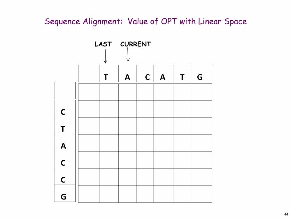
Sequence Alignment: Value of OPT with Linear Space
Sequence-Alignment(m, n, x1x2...xm, y1y2...yn, , ) {
for i = 0 to m
CURRENT[i] = i
for j = 1 to n
LASTCURRENT ( vector copy)
CURRENT[0] j
for i = 1 to m
CURRENT[i] min( [xi, yj] + LAST[i-1],
+ LAST[i],
+ CURRENT[i-1] )
return CURRENT[m]
}
• Two vectors of of m positions: LAST e CURRENT
• O(mn) time and O(m+n) space
44
Sequence Alignment: Value of OPT with Linear Space
LAST CURRENT
C
T
A
C
C
G
T A C A T G

45
Sequence Alignment: Algorithm for recovering the sequence
Analysis. (mn) space and O(m+n) time
Find_Sequence (i, j, x1x2...xm, y1y2...yn, , ) {
If i=0 or j=0 return
Else
If M[i, j] = [xi, yj] + M[i-1, j-1]
Add pair xi – yj to the solution
Return Find_Sequence(i-1,j-1)
Else If M[i,j]= + M[i-1, j]
Return Find_sequence(i-1,j)
Else return Find_sequence(i,j-1)
}
46
Sequence Alignment: Linear Space
Q. Can we avoid using quadratic space?
Easy. Optimal value in O(m + n) space and O(mn) time.
Compute OPT(i, •) from OPT(i-1, •).
No longer a simple way to recover alignment itself.
Theorem. [Hirschberg 1975] Optimal alignment in O(m + n) space and
O(mn) time.
Clever combination of divide-and-conquer and dynamic programming.
Inspired by idea of Savitch from complexity theory.

47
Edit distance graph.
Let f(i, j) be shortest path from (0,0) to (i, j).
Observation: f(i, j) = OPT(i, j).
Sequence Alignment: Linear Space
i-j
m-n
x1
x2
y1
x3
y2 y3 y4 y5 y6
0-0
xiy j

48
Edit distance graph.
Let f(i, j) be shortest path from (0,0) to (i, j).
Can compute f (•, j) for any j in O(mn) time and O(m + n) space.
Sequence Alignment: Linear Space
i-j
m-n
x1
x2
y1
x3
y2 y3 y4 y5 y6
0-0
j

49
Edit distance graph.
Let g(i, j) be shortest path from (i, j) to (m, n).
Can compute by reversing the edge orientations and inverting the
roles of (0, 0) and (m, n).
Sequence Alignment: Linear Space
i-j
m-n
x1
x2
y1
x3
y2 y3 y4 y5 y6
0-0
xiy j

50
Edit distance graph.
Let g(i, j) be shortest path from (i, j) to (m, n).
Can compute g(•, j) for any j in O(mn) time and O(m + n) space.
Sequence Alignment: Linear Space
i-j
m-n
x1
x2
y1
x3
y2 y3 y4 y5 y6
0-0
j

51
Observation 1. The cost of the shortest path that uses (i, j) is
f(i, j) + g(i, j).
Sequence Alignment: Linear Space
i-j
m-n
x1
x2
y1
x3
y2 y3 y4 y5 y6
0-0

52
Observation 2. let q be an index that minimizes f(q, n/2) + g(q, n/2).
Then, the shortest path from (0, 0) to (m, n) uses (q, n/2).
Sequence Alignment: Linear Space
i-j
m-n
x1
x2
y1
x3
y2 y3 y4 y5 y6
0-0
n / 2
q

53
Divide: find some index q that minimizes f(q, n/2) + g(q, n/2) using DP.
Align xq and yn/2.
Conquer: recursively compute optimal alignment in each piece.
Sequence Alignment: Linear Space
i-j x1
x2
y1
x3
y2 y3 y4 y5 y6
0-0
q
n / 2
m-n

54
Theorem. Let T(m, n) = max running time of algorithm on strings of
length at most m and n. T(m, n) = O(mn log n).
Remark. Analysis is not tight because two sub-problems are of size
(q, n/2) and (m - q, n/2). In next slide, we save log n factor.
Sequence Alignment: Running Time Analysis Warmup
T(m, n) 2T(m, n/2) O(mn) T(m, n) O(mn logn)

55
Theorem. Let T(m, n) = max running time of algorithm on strings of
length m and n. T(m, n) = O(mn).
Pf. (by induction on n)
O(mn) time to compute f( •, n/2) and g ( •, n/2) and find index q.
T(q, n/2) + T(m - q, n/2) time for two recursive calls.
Choose constant c so that:
Base cases: m = 2 or n = 2.
Inductive hypothesis: T(m, n) 2cmn.
Sequence Alignment: Running Time Analysis
cmn
cmncqncmncqn
cmnnqmccqn
cmnnqmTnqTnmT
2
2/)(22/2
)2/,()2/,(),(
T(m, 2) cm
T(2, n) cn
T(m, n) cmn T(q, n /2) T(m q, n /2)