Embed Size (px)
Citation preview
1
Chapter 6Information Theory
2
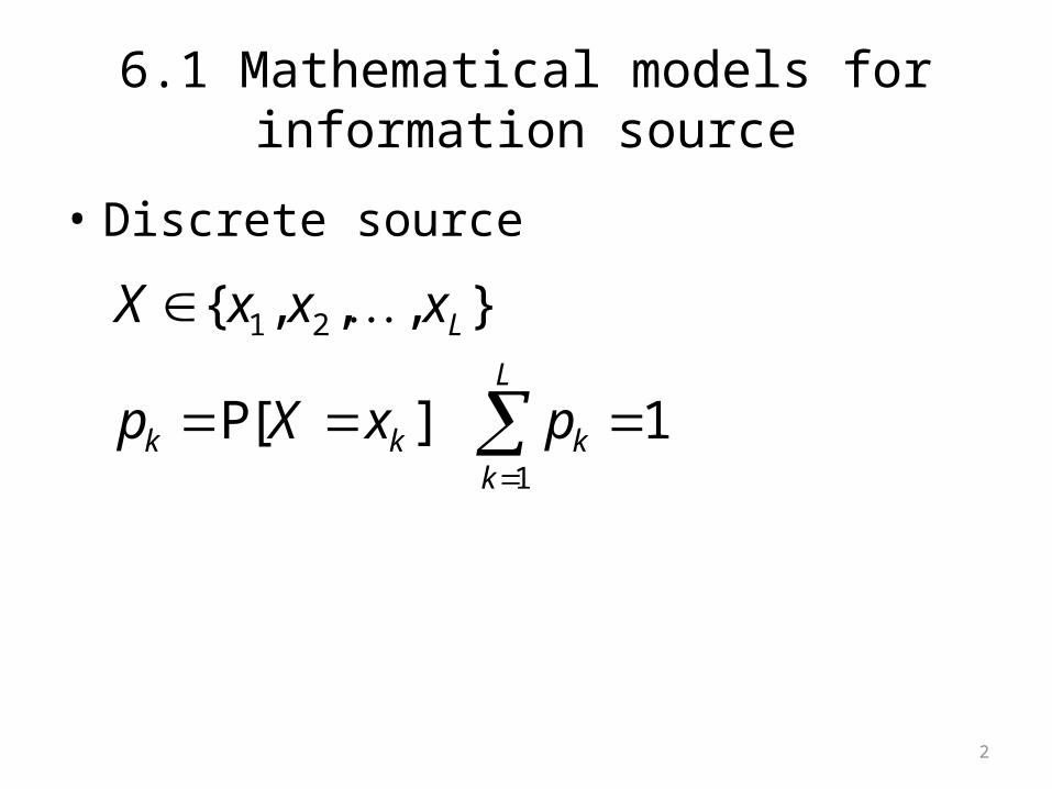
6.1 Mathematical models for information source
• Discrete source
1][P
},,,{
1
21
L
kkkk
L
pxXp
xxxX

3
6.1 Mathematical models for information source
• Discrete memoryless source (DMS)Source outputs are independent random variables
• Discrete stationary source– Source outputs are statistically dependent– Stationary: joint probabilities of and are identical for all shifts m– Characterized by joint PDF
NiX i ,,2,1}{
),,( 21 mxxxp
nxxx ,, 21
mnmm xxx ,, 21

4
6.2 Measure of information
• Entropy of random variable X– A measure of uncertainty or ambiguity in X
– A measure of information that is required by knowledge of X, or information content of X per symbol
– Unit: bits (log_2) or nats (log_e) per symbol – We define– Entropy depends on probabilities of X, not values of X
L
kkk
L
xXxXXH
xxxX
1
21
][Plog]P[)(
},,,{
00log0

5
Shannon’s fundamental paper in 1948“A Mathematical Theory of Communication”
Can we define a quantity which will measure how much information is “produced” by a process?
He wants this measure to satisfy:1) H should be continuous in 2) If all are equal, H should be monotonically
increasing with n3) If a choice can be broken down into two
successive choices, the original H should be the weighted sum of the individual values of H
),,,( 21 npppH
ipip

6
Shannon’s fundamental paper in 1948“A Mathematical Theory of Communication”
)3
1,
3
2(
2
1)
2
1,
2
1()
6
1,
3
1,
2
1( HHH

7
Shannon’s fundamental paper in 1948“A Mathematical Theory of Communication”
The only H satisfying the three assumptions is of the form:
K is a positive constant.
n
iii ppKH
1
log

8
Binary entropy function)1log()1(log)( ppppXH
H(p)
Probability p
H=0: no uncertaintyH=1: most uncertainty 1 bit for binary information

9
Mutual information• Two discrete random variables: X and Y
• Measures the information knowing either variables provides about the other
• What if X and Y are fully independent or dependent?
][P][P
],[Plog],[P
][P
]|[Plog],[P
),(],[P);(
yx
yxyYxX
x
yxyYxX
yxIyYxXYXI

10
),()()(
)|()(
)|()();(
YXHYHXH
XYHYH
YXHXHYXI
11
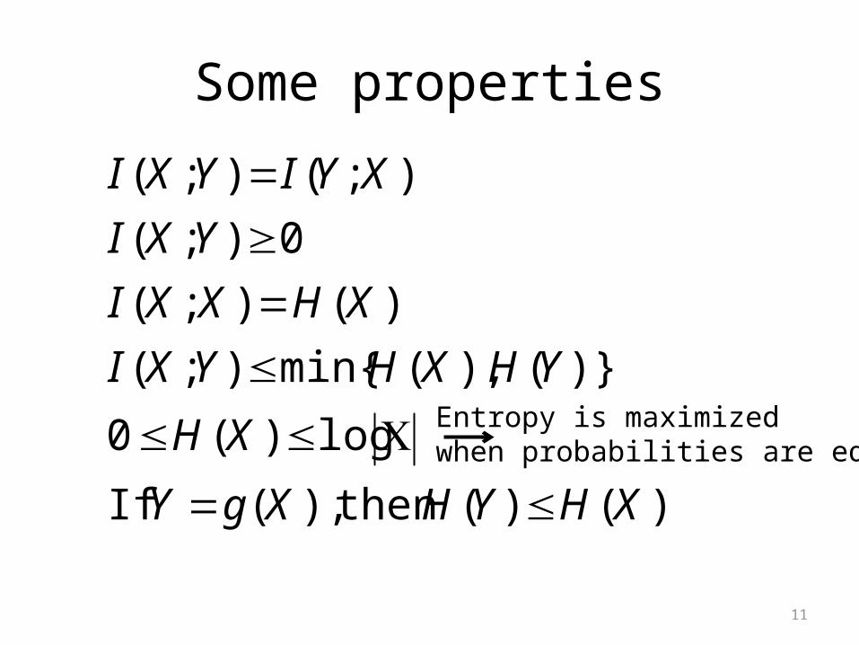
Some properties
)()(then),(If
log)(0
)}(),(min{);(
)();(
0);(
);();(
XHYHXgY
XH
YHXHYXI
XHXXI
YXI
XYIYXI
Entropy is maximized when probabilities are equal

12
Joint and conditional entropy
• Joint entropy
• Conditional entropy of Y given X
],[Plog],[P),( yYxXyYxXYXH
]|[log],[P
)|(][P)|(
xXyYPyYxX
xXYHxXXYH

13
Joint and conditional entropy
• Chain rule for entropies
• Therefore,
• If Xi are iid
),,,(
),|()|()(),,,(
121
21312121
nn
n
XXXXH
XXXHXXHXHXXXH
n
iin XHXXXH
121 )(),,,(
)(),,,( 21 XnHXXXH n
14
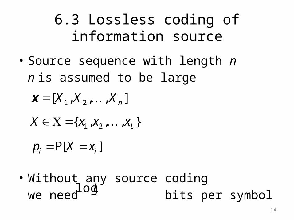
6.3 Lossless coding of information source
• Source sequence with length nn is assumed to be large
• Without any source codingwe need bits per symbol
},,,{ 21 LxxxX
],,,[ 21 nXXX x
][P ii xXp
Llog
15
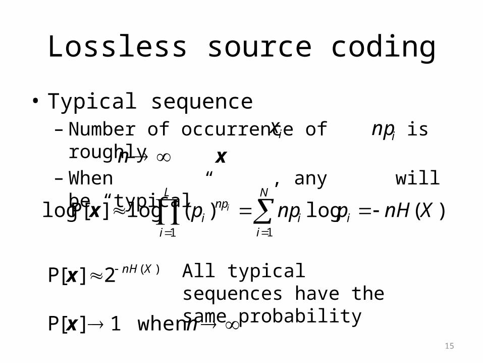
Lossless source coding
• Typical sequence– Number of occurrence of is roughly – When , any will be “typical”
ix inpn x
)(log)(log][Plog11
XnHpnppN
iii
L
i
npi
i
x
)(2][P XnHx All typical sequences have the same probability
nwhen1][P x

16
Lossless source coding
• Typical sequence
• Since typical sequences are almost certain to occur, for the source output it is sufficient to consider only these typical sequences
• How many bits per symbol we need now?
Number of typical sequences = )(2][P
1 XnHx
LXHn
XnHR log)(
)(

17
Lossless source coding
Shannon’s First Theorem - Lossless Source Coding
Let X denote a discrete memoryless source. There exists a lossless source code at rate R if
)(XHR bits per transmission

18
Lossless source coding
For discrete stationary source…
),,,|(lim
),,,(1
lim
)(
121
21
kkk
kk
XXXXH
XXXHk
XHR

19
Lossless source coding algorithms
• Variable-length coding algorithm– Symbols with higher probability are assigned
shorter code words
– E.g. Huffman coding• Fixed-length coding algorithm
E.g. Lempel-Ziv coding
)(min1
}{k
L
kk
nxPnR
k

20
Huffman coding algorithmP(x1)
P(x2)
P(x3)
P(x4)
P(x5)P(x6)
P(x7)
x1 00
x2 01
x3 10
x4 110
x5 1110
x6 11110
x7 11111
H(X)=2.11R=2.21 bits per symbol

21
6.5 Channel models and channel capacity
• Channel modelsinput sequenceoutput sequence
A channel is memoryless if
),,,(
),,,(
21
21
n
n
yyy
xxx
y
x
n
iii xy
1
]|[P]|[P xy

22
Binary symmetric channel (BSC) model
Channel encoder
Binary modulator Channel Demodulator
and detectorChannel decoder
Source data
Output data
Composite discrete-input discrete output channel

23
Binary symmetric channel (BSC) model
0 0
1 1
1-p
1-p
p
pInput Output
pXYPXY
pXYPXY
1]0|0[]1|1[P
]0|1[]1|0[P
24
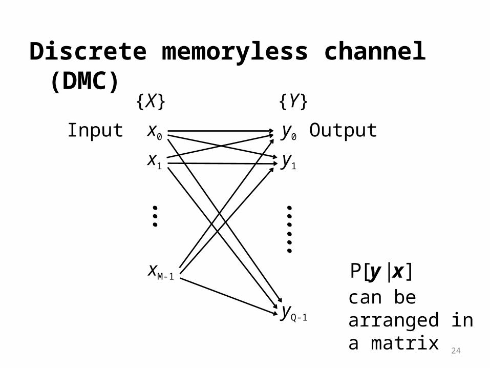
Discrete memoryless channel (DMC)
x0Input Outputx1
xM-1
…
y0
y1
yQ-1
……
{X} {Y}
]|[P xycan be arranged in a matrix
25
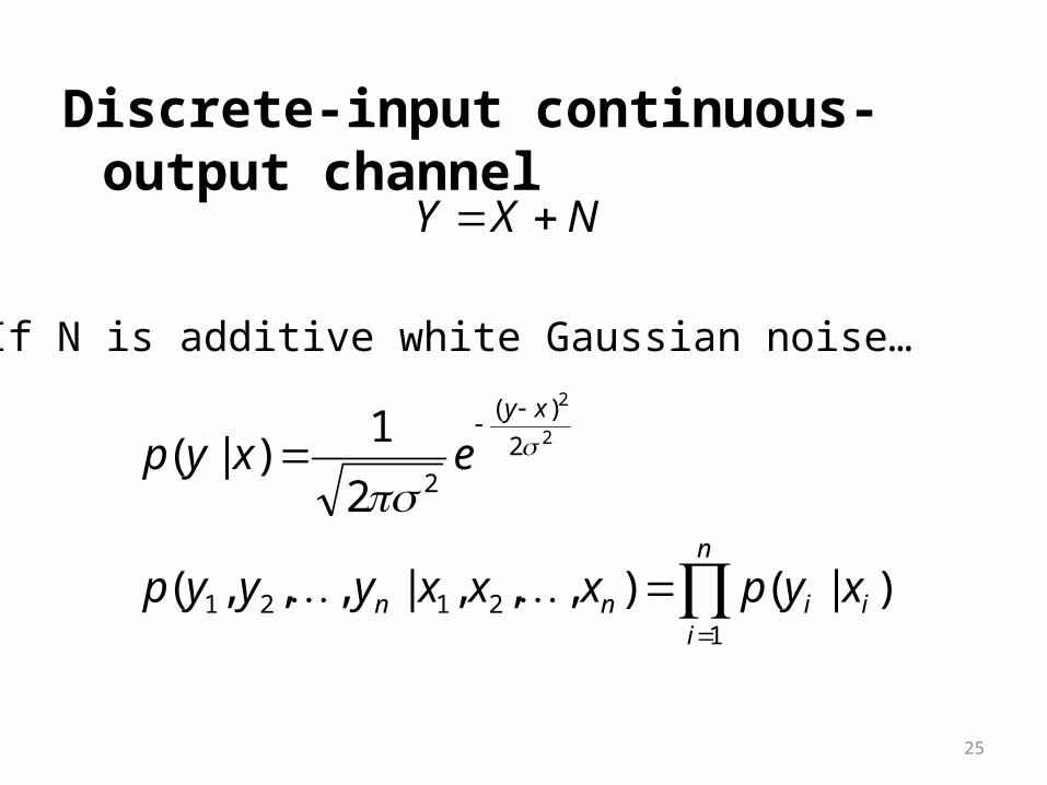
Discrete-input continuous-output channel
NXY
n
iiinn
xy
xypxxxyyyp
exyp
12121
2
)(
2
)|(),,,|,,,(
2
1)|(
2
2
If N is additive white Gaussian noise…

26
Discrete-time AWGN channel
• Power constraint• For input sequence with large
n
iii nxy
PX ][E 2
),,,( 21 nxxx x
Pn
xn
n
ii
2
1
2 11x

27
AWGN waveform channel
• Assume channel has bandwidth W, with frequency response C(f)=1, [-W, +W]
Channel encoder Modulator Physical
channelDemodulator and detector
Channel decoder
Source data
Output data
Input waveform
Output waveform
)()()( tntxty
28
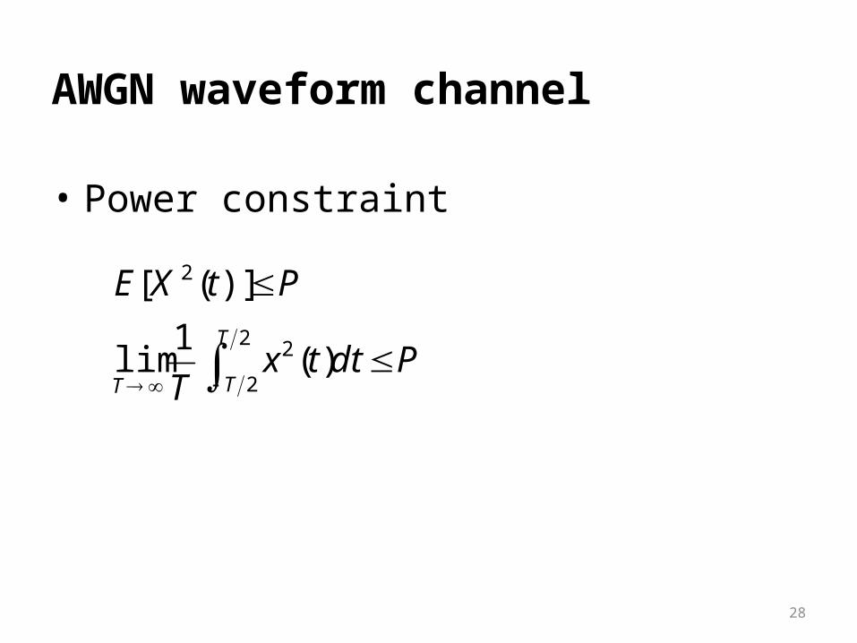
AWGN waveform channel
• Power constraint
PdttxT
PtXET
TT
2
2
2
2
)(1
lim
)]([

29
AWGN waveform channel
• How to define probabilities that characterize the channel?
jjj
jjj
jjj
tyty
tntn
txtx
)()(
)()(
)()(
jji nxy
Equivalent to 2W uses per second of a discrete-time channel }2,,2,1),({ WTjtj

30
AWGN waveform channel
• Power constraint becomes...
• Hence,P
XW
XWTT
xT
dttxT T
WT
jj
T
T
TT
][E2
][E21
lim1
lim)(1
lim
2
22
1
22
2
2
W
PXE
2][ 2
31
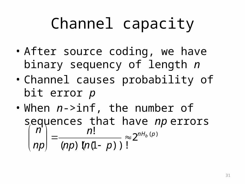
Channel capacity
• After source coding, we have binary sequency of length n
• Channel causes probability of bit error p• When n->inf, the number of sequences that
have np errors
)(2))!1(()!(
! pnHb
pnnp
n
np
n
32
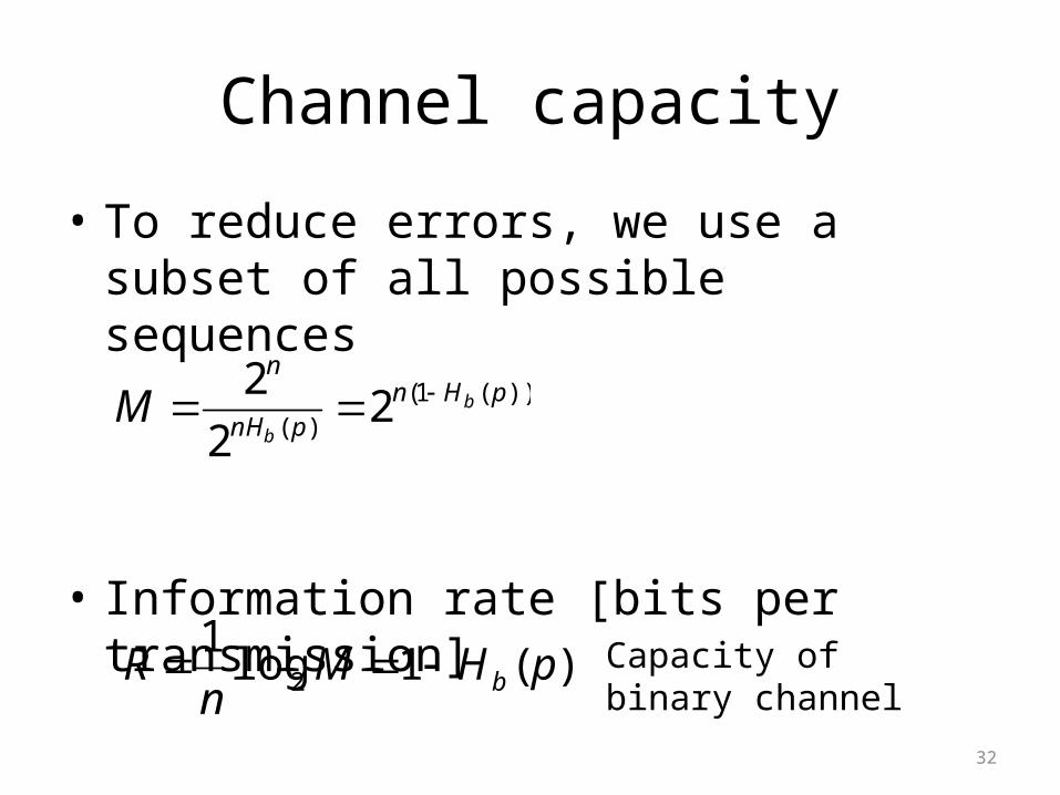
Channel capacity
• To reduce errors, we use a subset of all possible sequences
• Information rate [bits per transmission]
))(1()( 2
2
2 pHnpnH
nb
bM
)(1log1
2 pHMn
R b Capacity of binary channel

33
Channel capacity
We use 2m different binary sequencies of length m for transmission
2n different binary sequencies of length n contain information
1)(10 pHR bWe cannot transmit more than 1 bit per channel use
Channel encoder: add redundancy

34
Channel capacity
• Capacity for abitray discrete memoryless channel
• Maximize mutual information between input and output, over all
• Shannon’s Second Theorem – noisy channel coding- R < C, reliable communication is possible- R > C, reliable communication is impossible
);(max YXICp
),,,( 21 Xpppp

35
Channel capacity
For binary symmetric channel2
1]0[P]1[P XX
)(1)1(2log)1(2log1 pHppppC
36
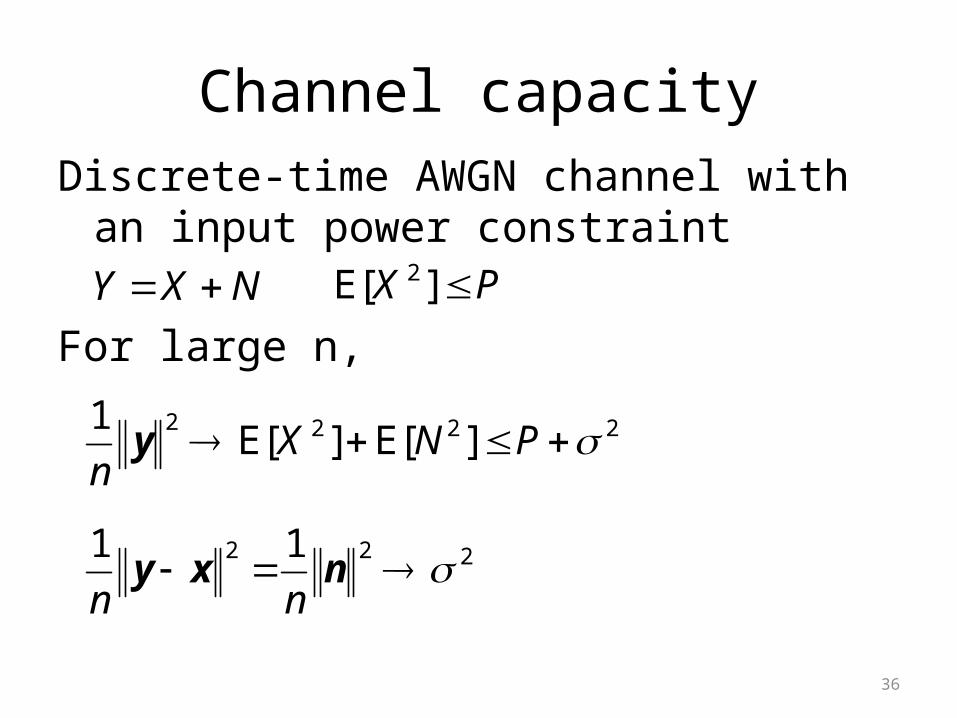
Channel capacityDiscrete-time AWGN channel with an input
power constraint
For large n, NXY PX ][E 2
2222][E][E
1 PNXny
222 11 nxynn

37
Channel capacityDiscrete-time AWGN channel with an input
power constraint
Maximum number of symbols to transmit
Transmission rate
NXY PX ][E 2
22
2
2
)1()( n
n
n
P
n
PnM
)1(log2
1log
1222 P
Mn
R Can be obtained by directly maximizing I(X;Y), subject to power constraint

38
Channel capacityBand-limited waveform AWGN channel with
input power constraint- Equivalent to 2W use per second of discrete-
time channel
)1(log2
1)
2
21(log2
1
02
02 WN
PNWP
C bits/channel use
)1(log)1(log2
12
02
02 WN
PW
WN
PWC bits/s

39
Channel capacity
0
02
44.1
)1(log
N
PCW
CP
WN
PWC

40
Channel capacity• Bandwidth efficiency
• Relation of bandwidth efficiency and power efficiency
)1(log0
2 WN
P
W
Rr
R
P
M
PT
Ms
b 22 loglog
)1(log)1(log0
20
2 Nr
WN
Rr bb
dB6.12ln,00
N
r brN
rb 12
0

41


