Chapter 6: CPU Scheduling · Operating System Concepts – 9 th Edition 6.3 Silberschatz, Galvin and Gagne ©2013 Objectives To introduce CPU scheduling, which is the basis for multiprogrammed

Silberschatz, Galvin and Gagne ©2013Operating System Concepts – 9th Edition

Chapter 6: CPU Scheduling

6.2 Silberschatz, Galvin and Gagne ©2013Operating System Concepts – 9th Edition

Chapter 6: CPU Scheduling

Basic Concepts Scheduling Criteria Scheduling Algorithms Thread Scheduling Multiple-Processor Scheduling Real-Time CPU Scheduling Operating Systems Examples Algorithm Evaluation


Objectives

To introduce CPU scheduling, which is the basis for multiprogrammed operating systems

To describe various CPU-scheduling algorithms To discuss evaluation criteria for selecting a CPU-scheduling

algorithm for a particular system To examine the scheduling algorithms of several operating

systems


BASIC CONCEPTS


Basic Concepts

Maximum CPU utilization obtained with multiprogramming

CPU–I/O Burst Cycle – Process execution consists of a cycle of CPU execution and I/O wait

CPU burst followed by I/O burst CPU burst distribution is of main

concern


CPU Scheduler

Short-term scheduler selects from among the processes inready queue, and allocates the CPU to one of them Queue may be ordered in various ways

CPU scheduling decisions may take place when a process:1. Switches from running to waiting state2. Switches from running to ready state3. Switches from waiting to ready4. Terminates

Scheduling under 1 and 4 is nonpreemptive All other scheduling is preemptive

Consider access to shared data Consider preemption while in kernel mode Consider interrupts occurring during crucial OS activities


Dispatcher

Dispatcher module gives control of the CPU to the process selected by the short-term scheduler; this involves: switching context switching to user mode jumping to the proper location in the user program to

restart that program Dispatch latency – time it takes for the dispatcher to stop

one process and start another running


SCHEDULING CRITERIA


Scheduling Criteria

CPU utilization – keep the CPU as busy as possible Throughput – # of processes that complete their execution per

time unit Turnaround time – amount of time to execute a particular

process Waiting time – amount of time a process has been waiting in the

ready queue Response time – amount of time it takes from when a request

was submitted until the first response is produced, not output (for time-sharing environment)


Scheduling Algorithm Optimization Criteria

Max CPU utilization Max throughput Min turnaround time Min waiting time Min response time

We are going to use the average waiting time to compare the following algorithms


SCHEDULING ALGORITHMS


First- Come, First-Served (FCFS) Scheduling

Process Burst TimeP1 24P2 3P3 3

Suppose that the processes arrive in the order: P1 , P2 , P3 The Gantt Chart for the schedule is:

Waiting time for P1 = 0; P2 = 24; P3 = 27 Average waiting time: (0 + 24 + 27)/3 = 17

P P P1 2 3

0 24 3027


FCFS Scheduling (Cont.)

Suppose that the processes arrive in the order:P2 , P3 , P1

The Gantt chart for the schedule is:

Waiting time for P1 = 6; P2 = 0; P3 = 3 Average waiting time: (6 + 0 + 3)/3 = 3 Much better than previous case Convoy effect - short process behind long process

Consider one CPU-bound and many I/O-bound processes

P10 3 6 30

P2 P3


Shortest-Job-First (SJF) Scheduling

Associate with each process the length of its next CPU burst Use these lengths to schedule the process with the shortest time

ProcessArriva l Time Burst TimeP1 0.0 6P2 2.0 8P3 4.0 7P4 5.0 3

SJF scheduling chart

Average waiting time = (3 + 16 + 9 + 0) / 4 = 7

P30 3 24

P4 P1169

P2


Shortest-Job-First (SJF) Scheduling

SJF is optimal – gives minimum average waiting time for a given set of processes The difficulty is knowing the length of the next CPU request Could ask the user

SJF can be preemptive and nonpreemptive considering he new coming processes Preemptive version called shortest-remaining-time-first


Determining Length of Next CPU Burst

Can only estimate the length – should be similar to the previous one Then pick process with shortest predicted next CPU burst

Can be done by using the length of previous CPU bursts, using exponential averaging

Commonly, α set to ½ and =10

:Define 4.10 , 3.

burst CPU next the for value predicted 2.burst CPU of length actual 1.

1n

thn nt

.11 nnn t

0


Prediction of the Length of the Next CPU Burst


Examples of Exponential Averaging

=0 n+1 = n

Recent history does not count =1

n+1 = tn Only the actual last CPU burst counts

If we expand the formula, we get:n+1 = tn+(1 - ) tn -1 + …

+(1 - )j tn -j + …+(1 - )n +1 0

Since both and (1 - ) are less than or equal to 1, each successive term has less weight than its predecessor


Example of Shortest-remaining-time-first

Now we add the concepts of varying arrival times and preemption to the analysis

ProcessAarri Arrival TimeT Burst TimeP1 0 8P2 1 4P3 2 9P4 3 5

Preemptive SJF Gantt Chart

Average waiting time = [(10-1)+(1-1)+(17-2)+5-3)]/4 = 26/4 = 6.5 msec

P40 1 26

P1 P210

P3P15 17


Priority Scheduling

A priority number (integer) is associated with each process

The CPU is allocated to the process with the highest priority (smallest integer highest priority) Preemptive Nonpreemptive

SJF is priority scheduling where priority is the inverse of predicted next CPU burst time

Problem Starvation – low priority processes may never execute Solution Aging – as time progresses increase the priority of

the process


Example of Priority Scheduling (nonpreemptive)

ProcessA arri Burst TimeT PriorityP1 10 3P2 1 1P3 2 4P4 1 5P5 5 2

Priority scheduling Gantt Chart

Average waiting time = 8.2 msec

1

0 1 19

P1 P216

P4P36 18

P


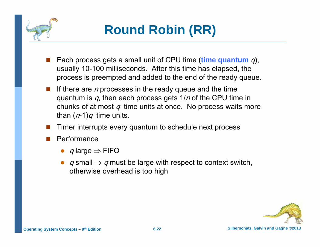
Round Robin (RR)

Each process gets a small unit of CPU time (time quantum q), usually 10-100 milliseconds. After this time has elapsed, the process is preempted and added to the end of the ready queue.

If there are n processes in the ready queue and the time quantum is q, then each process gets 1/n of the CPU time in chunks of at most q time units at once. No process waits more than (n-1)q time units.

Timer interrupts every quantum to schedule next process Performance

q large FIFO q small q must be large with respect to context switch,

otherwise overhead is too high


Example of RR with Time Quantum = 4

Process Burst TimeP1 24P2 3P3 3

The Gantt chart is:

Typically, higher average turnaround than SJF, but better response

P P P1 1 1

0 18 3026144 7 10 22

P2 P3 P1 P1 P1


Time Quantum and Context Switch Time

q should be large compared to context switch time q usually 10ms to 100ms, context switch < 10 usec


Turnaround Time Varies With The Time Quantum

80% of CPU bursts should be shorter than q


Multilevel Queue

Ready queue is partitioned into separate queues, eg: foreground (interactive) background (batch)

Process permanently in a given queue Each queue has its own scheduling algorithm:

foreground – RR background – FCFS

Scheduling must be done between the queues: Fixed priority scheduling; (i.e., serve all from foreground then

from background). Possibility of starvation. Time slice – each queue gets a certain amount of CPU time

which it can schedule amongst its processes; i.e., 80% to foreground in RR

20% to background in FCFS


Multilevel Queue Scheduling


Multilevel Feedback Queue

A process can move between the various queues; aging can be implemented this way

Three queues: Q0 – RR with time quantum 8 milliseconds Q1 – RR time quantum 16 milliseconds Q2 – FCFS

Scheduling A new job enters queue Q0 which is served FCFS

When it gains CPU, job receives 8 milliseconds If it does not finish in 8 milliseconds, job is moved to queue Q1

At Q1 job is again served FCFS and receives 16 additional milliseconds If it still does not complete, it is preempted and moved to queue Q2


Multilevel Feedback Queue

Multilevel-feedback-queue scheduler defined by the following parameters: number of queues scheduling algorithms for each queue method used to determine when to upgrade a process method used to determine when to demote a process method used to determine which queue a process will enter

when that process needs service


SCHEDULING FOR DIFFERENT TECHNIQUES


Thread Scheduling

Distinction between user-level and kernel-level threads When threads supported, threads scheduled, not processes Many-to-one and many-to-many models, thread library schedules

user-level threads to run on LWP Known as process-contention scope (PCS) since scheduling

competition is within the process Typically done via priority set by programmer

Kernel thread scheduled onto available CPU is system-contention scope (SCS) – competition among all threads in system


Multiple-Processor Scheduling

CPU scheduling more complex when multiple CPUs are available

Homogeneous processors within a multiprocessor

Asymmetric multiprocessing – only one processor accesses the system data structures, alleviating the need for data sharing

Symmetric multiprocessing (SMP) – each processor is self-scheduling, all processes in common ready queue, or each has its own private queue of ready processes Currently, most common


Multiple-Processor Scheduling – Processor affinity

Processor affinity – process has affinity for processor on which it is currently running soft affinity hard affinity Variations including processor sets

Note that memory-placement algorithms can also consider affinity


Multiple-Processor Scheduling – Load Balancing

If SMP, need to keep all CPUs loaded for efficiency Load balancing attempts to keep workload evenly distributed

Push migration – periodic task checks load on each processor, and if found pushes task from overloaded CPU to other CPUs

Pull migration – idle processors pulls waiting task from busy processor

Load balancing solution techniques destroy the affinity concept


Multicore Processors

Recent trend to place multiple processor cores on same physical chip

Faster and consumes less power Multiple threads per core also growing

Takes advantage of memory stall to make progress on another thread while memory retrieve happens


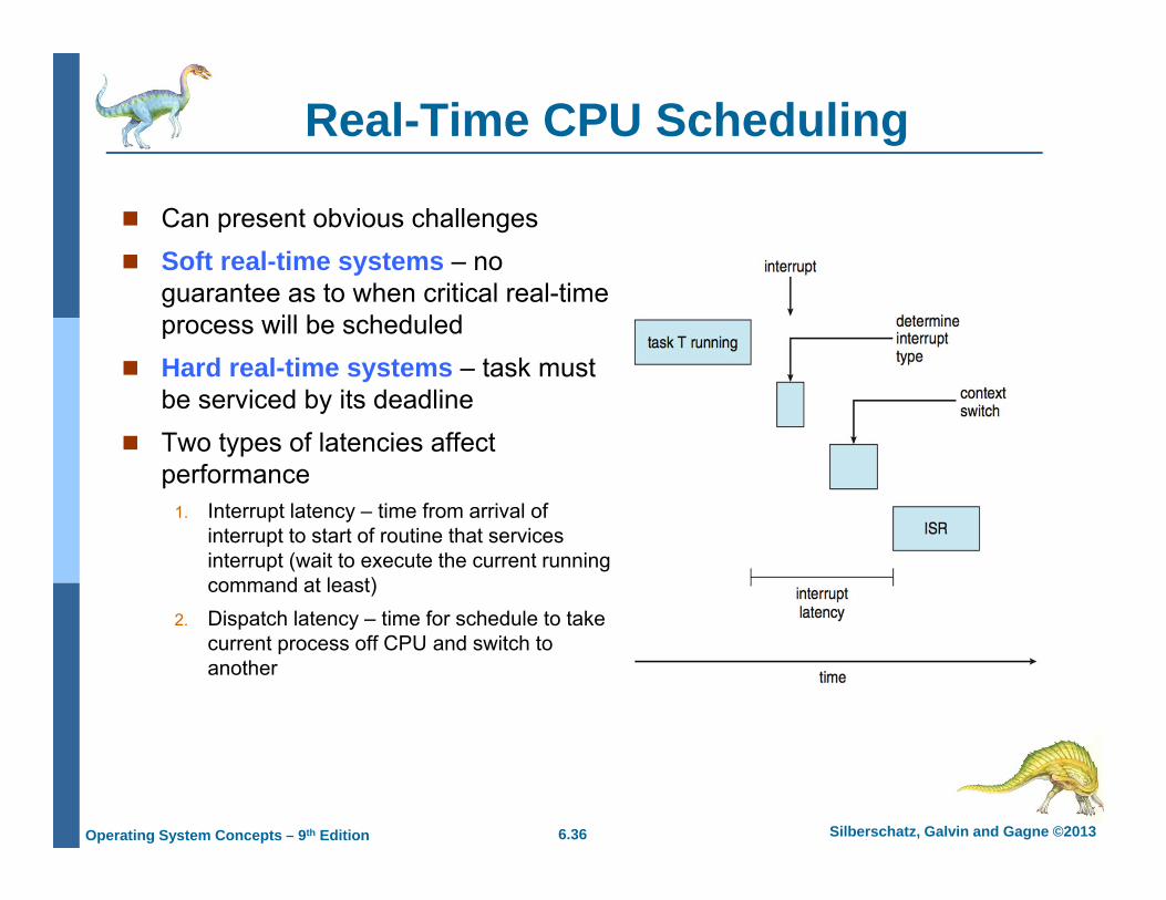
Real-Time CPU Scheduling

Can present obvious challenges Soft real-time systems – no

guarantee as to when critical real-time process will be scheduled

Hard real-time systems – task must be serviced by its deadline

Two types of latencies affect performance

1. Interrupt latency – time from arrival of interrupt to start of routine that services interrupt (wait to execute the current running command at least)

2. Dispatch latency – time for schedule to take current process off CPU and switch to another


Real-Time CPU Scheduling (Cont.)

Conflict phase of dispatch latency:

1. Preemption of any process running in kernel mode

2. Release low-priority process of resources needed by high-priority processes


Priority-based Scheduling

For real-time scheduling, scheduler must support preemptive, priority-based scheduling But only guarantees soft real-time

For hard real-time must also provide ability to meet deadlines Processes have new characteristics: periodic ones require CPU at

constant intervals Has processing time t, deadline d, period p 0 ≤ t ≤ d ≤ p Rate of periodic task is 1/p


Operating System Examples

Linux scheduling

Windows scheduling


Linux Scheduling

Prior to kernel version 2.5, ran variation of standard UNIX scheduling algorithm with no support for SMP

Version 2.6 moved to constant order O(1) scheduling time with support for SMP. Bus has bad performance for interactive desktop apps.

Version 2.6.23 introduce the Complete fair scheduling algorithm (CFS) with the following criteria Max time specified with the complete fair concept manipulate a red-black tree instead of a queue. Preemptive, static priority based Two priority classes: time-sharing and real-time Priority with numerically lower values indicating higher priority

Version 2.6.24 initialize new time-sharing tasks with vruntime calculated based on a nice value in the range [-20 to 19] Time-sharing class mapped the nice value to dynamic priorities in the

range [100 to 139] Real-time class has static priorities in the range [0 to 99]


CFS Performance


Linux Scheduling (Cont.)

Real-time scheduling according to POSIX.1b Real-time tasks have static priorities

Real-time plus normal map into global priority scheme Nice value of -20 maps to global priority 100 Nice value of +19 maps to priority 139


Windows Scheduling

The Scheduler called Dispatcher in Windows Windows uses priority-based preemptive scheduling Highest-priority thread runs next Thread runs until (1) terminates, (2) uses time slice, (3)

preempted by higher-priority thread Real-time threads can preempt non-real-time 32-level priority scheme Variable class is 1-15, real-time class is 16-31 Priority 0 is memory-management thread Queue for each priority If no run-able thread, runs idle thread


Windows Priority Classes

Win32 API identifies several priority classes to which a process can belong REALTIME_PRIORITY_CLASS, HIGH_PRIORITY_CLASS,

ABOVE_NORMAL_PRIORITY_CLASS,NORMAL_PRIORITY_CLASS, BELOW_NORMAL_PRIORITY_CLASS, IDLE_PRIORITY_CLASS

All are variable except REALTIME

A thread within a given priority class has a relative priority TIME_CRITICAL, HIGHEST, ABOVE_NORMAL, NORMAL, BELOW_NORMAL,

LOWEST, IDLE

Priority class and relative priority combine to give numeric priority Base priority is NORMAL within the class If quantum expires, priority lowered, but never below base


Windows Priorities


Windows Priority Classes (Cont.)

If wait occurs, priority boosted depending on what was waited for Foreground window given 3x priority boost Windows 7 added user-mode scheduling (UMS)

Applications create and manage threads independent of kernel For large number of threads, much more efficient UMS schedulers come from programming language libraries like

C++ Concurrent Runtime (ConcRT) framework


ACCESS SCHEDULING IN USER LEVEL


POSIX pthread scheduling

http://sallamah.weebly.com/uploads/6/9/3/5/6935631/posixsched.c

Silberschatz, Galvin and Gagne ©2013Operating System Concepts – 9th Edition

End of Chapter 6

Documents

Chapter 6: CPU Scheduling · Operating System Concepts – 9 th Edition 6.3 Silberschatz, Galvin and Gagne ©2013 Objectives To introduce CPU scheduling, which is the basis for multiprogrammed