Chapter 6 Basics of Digital Audio 6.1 Digitization of Sound 6.3 Quantization and Transmission of Audio 1 IT342

Chapter 6Basics of Digital Audio

6.1 Digitization of Sound6.3 Quantization and Transmission of Audio

1

IT34

2

IT34

2

Fundamentals of Multimedia, Chapter 6

6.1 Digitization of Sound

What is Sound?• Sound is a wave phenomenon like light, but is macroscopic

and involves molecules of air being compressed and expanded under the action of some physical device.• For example, a speaker in an audio system vibrates back and

forth and produces a longitudinal pressure wave that we perceive as sound.

• Without air there is no sound. Since sound is a pressure wave, it takes on continuous values, as opposed to digitized ones.

• If we want to use a digital version of sound wave, we must form digitized representations of audio information.

2

IT34

2


• Even though such pressure waves are longitudinal, they still have ordinary wave properties and behaviors, such as reflection (bouncing), refraction (change of angle when entering a medium with a different density) and diffraction (bending around an obstacle).

• Since sound consists of measurable pressures at any 3D point, we can detect it by measuring the pressure level at location, using transducer to convert pressure to voltage levels.

3

IT34

2


Digitization• Digitization means conversion to a stream of numbers, and

preferably these numbers should be integers for efficiency.• Fig. 6.1 shows the 1-dimensional nature of sound: amplitude

values depend on a 1D variable, time. i.e. the pressure increase or decreases with time. (And note that images depend instead on a 2D set of variables, x and y).

• The amplitude value is a continuous quantity in order to work with such data in computer storage we must digitize the analog signals.

4

IT34

2


• Fig. 6.1: An analog signal: continuous measurement of pressure wave. 5

IT34

2


• The graph in Fig. 6.1 has to be made digital in both time and amplitude. To digitize, the signal must be sampled in each dimension: in time, and in amplitude.• Sampling means measuring the quantity we are interested in, usually

at evenly-spaced intervals.• The first kind of sampling, using measurements only at evenly

spaced time intervals, is simply called, sampling. The rate at which it is performed is called the sampling frequency (see Fig. 4.2(a)).

• For audio, typical sampling rates are from 8 kHz (8,000 samples per second) to 48 kHz. This range is determined by the Nyquist theorem.

• Sampling in the amplitude or voltage dimension is called quantization. Fig. 4.2(b) shows this kind of sampling.

6

IT34

2


•Fig. 6.2: Sampling and Quantization. (a): Sampling the analog signal in the time dimension. (b): Quantization is sampling the analog signal in the amplitude dimension. 7

(a) (b)

IT34

2


• Typical uniform quantization rates are 8-bit and 16-bit; 8-bit quantization divides the vertical axis into 256 levels, and 16-bit divides it into 65,536 levels.

• Thus to decide how to digitize audio data we need to answer the following questions:• What is the sampling rate?• How finely is the data to be quantized, and is quantization uniform?• How is audio data formatted? (file format)

8

IT34

2


• Signals can be decomposed into a sum of sinusoids.

• Figure shows how weighted sinusoids can build up quite a complex signal.

9

Nyquist Theorem

IT34

2


• The Nyquist theorem states how frequently we must sampling time to be able to recover the original sound.• Fig. 6.3(a) shows a single sinusoid: it is a single, pure, frequency

(only electronic instruments can create such sounds).• If sampling rate just equals the actual frequency, Fig. 6.3(b) shows

that a false signal is detected: it is simply a constant, with zero frequency.

• Now if sample at 1.5 times the actual frequency, Fig. 6.3(c) shows that we obtain an incorrect (alias) frequency that is lower than the correct one — it is half the correct one (the wavelength, from peak to peak, is double that of the actual signal).

• Thus for correct sampling we must use a sampling rate equal to at least twice the maximum frequency content in the signal. This rate is called the Nyquist rate.

10

IT34

2


11

Fig. 6.3: Aliasing.

(a): A single frequency.

(b): Sampling at exactly the frequency produces a constant.

(c): Sampling at 1.5 times per cycle produces an alias perceived frequency.

IT34

2


• Nyquist Theorem: If a signal is band-limited, i.e., there is a lower limit f1 and an upper limit f2 of frequency components in the signal, then the sampling rate should be at least 2(f2 − f1).

• Nyquist frequency: half of the Nyquist rate.• Since it would be impossible to recover frequencies higher than

Nyquist frequency in any event, most systems have an antialiasing filter that restricts the frequency content in the input to the sampler to a range at or below Nyquist frequency.

• The relationship among the Sampling Frequency, True Frequency, and the Alias Frequency is as follows:• falias = fsampling − ftrue, for ftrue < fsampling < 2 × ftrue

(4.1)

12

IT34

2


Signal to Noise Ratio (SNR)• Random fluctuations in any analog system (noise)• The ratio of the power of the correct signal and the noise is called

the signal to noise ratio (SNR) — a measure of the quality of the signal.

• The SNR is usually measured in decibels (dB), where 1 dB is a tenth of a bel. The SNR value, in units of dB, is defined in terms of base-10 logarithms of squared voltages, as follows:

(6.2)

• 13

2

10 10210log 20logsignal signal

noise noise

V VSNR

V V

IT34

2


• The power in a signal is proportional to the square of the voltage. For example, if the signal voltage Vsignal is 10 times the noise, then the SNR is 20 log∗ 10(10) = 20dB.

• In terms of power, if the power from ten violins is ten times that from one violin playing, then the ratio of power is 10dB, or 1B.

• To know: Power — 10; Signal Voltage — 20.

14

IT34

2


• The usual levels of sound we hear around us are described in terms of decibels, as a ratio to the quietest sound we are capable of hearing. Table 6.1 shows approximate levels for these sounds.

• Table 6.1: Magnitude levels of common sounds, in decibels

• 15

Threshold of hearing 0

Rustle of leaves 10

Very quiet room 20

Average room 40

Conversation 60

Busy street 70

Loud radio 80

Train through station 90

Riveter 100

Threshold of discomfort 120

Threshold of pain 140

Damage to ear drum 160

IT34

2


Signal to Quantization Noise Ratio (SQNR)• For digital audio signals; where only quantized values are

stored; the precision of each sample is determined by the number of bits per sample, typically …..or…

• Aside from any noise that may have been present in the original analog signal, there is also an additional error that results from quantization.• If voltages are actually in 0 to 1 but we have only 8 bits in which

to store values, then effectively we force all continuous values of voltage into only 256 different values.

• This introduces a round off error. It is not really “noise”. Nevertheless it is called quantization noise (or quantization error).

16

IT34

2


• The quality of the quantization is characterized by the Signal to Quantization Noise Ratio (SQNR).• Quantization noise: the difference between the actual value of the

analog signal, for the particular sampling time, and the nearest quantization interval value.

• At most, this error can be as much as half of the interval.• For a quantization accuracy of N bits per sample, the SQNR can be

simply expressed:

17

1220log 20log

10 10 1_

2

20 log 2 6.02 (dB)

V NsignalSQNR

Vquan noise

N N

IT34

2


Linear and Non-linear Quantization

• Linear format: samples are typically stored as uniformly quantized values.

• Non-uniform quantization: set up more finely-spaced levels where humans hear with the most acuity.• Weber’s Law stated formally says that equally perceived differences

have values proportional to absolute levels:

ΔResponse ∝ ΔStimulus/Stimulus (6.5)

• Inserting a constant of proportionality k, we have a differentail equation that states:

dr = k (1/s) ds (6.6)• with response r and stimulus s.

18

IT34

2


Integrating, we arrive at a solution

r = k ln s + C (6.7)

with constant of integration C.Stated differently, the solution is

r = k ln(s/s0) (6.8)

s0 = the lowest level of stimulus that causes a response

(r = 0 when s = s0).

• Nonlinear quantization works by first transforming an analog signal from the raw s space into the theoretical r space, and then uniformly quantizing the resulting values.

• Such a law for audio is called μ-law encoding, (or u-law). A very similar rule, called A-law, is used in telephony in Europe.

• The equations for these very similar encodings are as follows: 19

IT34

2


• μ-law:

(6.9)

• A-law:

(6.10)

• Fig. 6.6 shows these curves. The parameter μ is set to μ = 100 or μ = 255; the parameter A for the A-law encoder is usually set to A = 87.6.

20

sgn( )ln 1 , 1

ln(1 ) p p

s s sr

s s

1,

1 ln

sgn( ) 11 ln , 1

1 ln

p p

p p

A s s

A s s A

r

s s sA

A s A s

1 if 0,where sgn( )

1 otherwise

ss

IT34

2


• Fig. 6.6: Nonlinear transform for audio signals• The μ-law in audio is used to develop a nonuniform quantization rule

for sound: uniform quantization of r gives finer resolution in s at the quiet end. 21

IT34

2


Audio Filtering• Prior to sampling and AD conversion, the audio signal is also

usually filtered to remove unwanted frequencies. The frequencies kept depend on the application:• For speech, typically from 50Hz to 10kHz is retained, and other

frequencies are blocked by the use of a band-pass filter that screens out lower and higher frequencies.

• An audio music signal will typically contain from about 20Hz up to 20kHz.

• At the DA converter end, high frequencies may reappear in the output — because of sampling and then quantization, smooth input signal is replaced by a series of step functions containing all possible frequencies.

• So at the decoder side, a lowpass filter is used after the DA circuit. 22

IT34

2


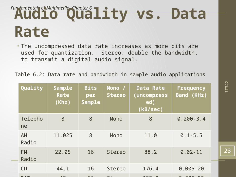
Audio Quality vs. Data Rate• The uncompressed data rate increases as more bits are used for

quantization. Stereo: double the bandwidth. to transmit a digital audio signal.

Table 6.2: Data rate and bandwidth in sample audio applications

•

•

23

Quality Sample Rate (Khz)

Bits per Sample

Mono / Stereo

Data Rate (uncompressed)

(kB/sec)

Frequency Band (KHz)

Telephone 8 8 Mono 8 0.200-3.4

AM Radio 11.025 8 Mono 11.0 0.1-5.5

FM Radio 22.05 16 Stereo 88.2 0.02-11

CD 44.1 16 Stereo 176.4 0.005-20

DAT 48 16 Stereo 192.0 0.005-20

DVD Audio 192 (max) 24(max) 6 channels

1,200 (max) 0-96 (max)

IT34

2


6.3 Quantization and Transmission of Audio

• Coding of Audio: Quantization and transformation of data are collectively known as coding of the data.• For audio, the μ-law technique for companding audio signals is usually

combined with an algorithm that exploits the temporal redundancy present in audio signals.

• Differences in signals between the present and a past time can reduce the size of signal values and also concentrate the histogram of pixel values (differences, now) into a much smaller range.

• The result of reducing the variance of values is that lossless compression methods produce a bitstream with shorter bit lengths for more likely values (→ expanded discussion in Chap.7).

• In general, producing quantized sampled output for audio is called PCM (Pulse Code Modulation). The differences version is called DPCM (and a crude but efficient variant is called DM). The adaptive version is called ADPCM.

24

IT34

2


Pulse Code Modulation• The basic techniques for creating digital signals from analog

signals are sampling and quantization.• Quantization consists of selecting breakpoints in magnitude, and

then re-mapping any value within an interval to one of the representative output levels. −→ Repeat of Fig. 6.2:• The set of interval boundaries are called decision boundaries, and

the representative values are called reconstruction levels.• The boundaries for quantizer input intervals that will all be mapped

into the same output level form a coder mapping.• The representative values that are the output values from a

quantizer are a decoder mapping.• Finally, we may wish to compress the data, by assigning a bit stream

that uses fewer bits for the most prevalent signal values 25

IT34

2


Fig. 6.2: Sampling and Quantization.

26

(a) (b)

IT34

2


• Every compression scheme has three stages:• The input data is transformed to a new representation that is easier

or more efficient to compress.• We may introduce loss of information. Quantization is the main lossy

step we use a limited number of reconstruction levels, fewer than ⇒in the original signal.

• Coding. Assign a codeword (thus forming a binary bitstream) to each output level or symbol. This could be a fixed-length code, or a variable length code such as Huffman coding.

• For audio signals, we first consider PCM for digitization. This leads to Lossless Predictive Coding as well as the DPCM scheme; both methods use differential coding. As well, we look at the adaptive version, ADPCM, which can provide better compression.

27

IT34

2


PCM in Speech Compression• Assuming a bandwidth for speech from about 50 Hz to about 10

kHz, the Nyquist rate would dictate a sampling rate of 20 kHz.• Using uniform quantization without companding, the minimum

sample size we could get away with would likely be about 12 bits. Hence for mono speech transmission the bit-rate would be 240 kbps.

• With companding, we can reduce the sample size down to about 8 bits with the same perceived level of quality, and thus reduce the bit-rate to 160 kbps.

• However, the standard approach to telephony in fact assumes that the highest-frequency audio signal we want to reproduce is only about 4 kHz. Therefore the sampling rate is only 8 kHz, and the companded bit-rate thus reduces this to 64 kbps.

28

IT34

2


• However, there are two small wrinkles we must also address:1. Since only sounds up to 4 kHz are to be considered, all other

frequency content must be noise. Therefore, we should remove this high-frequency content from the analog input signal. This is done using a band-limiting filter that blocks out high, as well as very low, frequencies. Also, once we arrive at a pulse signal, such as that in Fig. 6.13(a) below, we must still perform DA conversion and then construct a final output analog signal. But, effectively, the signal we arrive at is the staircase shown in Fig. 6.13(b).

2. A discontinuous signal contains not just frequency components due to the original signal, but also a theoretically infinite set of higher-frequency components:• This result is from the theory of Fourier analysis, in signal processing.• These higher frequencies are extraneous.• Therefore the output of the digital-to-analog converter goes to a low-pass

filter that allows only frequencies up to the original maximum to be retained.

29

IT34

2


Fig. 6.13: Pulse Code Modulation (PCM). (a) Original analog signal and its corresponding PCM signals. (b) Decoded staircase signal. (c) Reconstructed signal after low-pass filtering. 30

IT34

2


• The complete scheme for encoding and decoding telephony signals is shown as a schematic in Fig. 6.14. As a result of the low-pass filtering, the output becomes smoothed and Fig. 6.13(c) above showed this effect.

Fig. 6.14: PCM signal encoding and decoding.31

IT34

2


Differential Coding of Audio• Audio is often stored not in simple PCM but instead in a form

that exploits differences — which are generally smaller numbers, so offer the possibility of using fewer bits to store.• If a time-dependent signal has some consistency over time

(“temporal redundancy”), the difference signal, subtracting the current sample from the previous one, will have a more peaked histogram, with a maximum around zero.

• For example, as an extreme case the histogram for a linear ramp signal that has constant slope is flat, whereas the histogram for the derivative of the signal (i.e., the differences, from sampling point to sampling point) consists of a spike at the slope value.

• So if we then go on to assign bit-string codewords to differences, we can assign short codes to prevalent values and long codewords to rarely occurring ones.

32

IT34

2


Lossless Predictive Coding• Predictive coding: simply means transmitting differences — predict

the next sample as being equal to the current sample; send not the sample itself but the difference between previous and next.• Predictive coding consists of finding differences, and transmitting

these using a PCM system.• Note that differences of integers will be integers. Denote the integer

input signal as the set of values fn. Then we predict values as simply the previous value, and define the error en as the difference between the actual and the predicted signal:

(6.12)33

nf

1n n

n n n

f f

e f f

IT34

2


• But it is often the case that some function of a few of the previous

values, fn−1, fn−2, fn−3, etc., provides a better prediction. Typically, a linear predictor function is used:

(6.13)

34

2 to 4

1n n k n k

k

f a f

IT34

2


• The idea of forming differences is to make the histogram of sample values more peaked.• For example, Fig.6.15(a) plots 1 second of sampled speech at 8 kHz,

with magnitude resolution of 8 bits per sample.• A histogram of these values is actually centered around zero, as in

Fig. 6.15(b).• Fig. 6.15(c) shows the histogram for corresponding speech signal

differences: difference values are much more clustered around zero than are sample values themselves.

• As a result, a method that assigns short codewords to frequently occurring symbols will assign a short code to zero and do rather well: such a coding scheme will much more efficiently code sample differences than samples themselves.

35

IT34

2


•Fig. 6.15: Differencing concentrates the histogram. (a): Digital speech signal. (b): Histogram of digital speech signal values. (c): Histogram of digital speech signal differences. 36

IT34

2


• One problem: suppose our integer sample values are in the range 0..255. Then differences could be as much as -255..255 —we’ve increased our dynamic range (ratio of maximum to minimum) by a factor of two → need more bits to transmit some differences.• A clever solution for this: define two new codes, denoted SU and

SD, standing for Shift-Up and Shift-Down. Some special code values will be reserved for these.

• Then we can use codewords for only a limited set of signal differences, say only the range −15..16. Differences which lie in the limited range can be coded as is, but with the extra two values for SU, SD, a value outside the range −15..16 can be transmitted as a series of shifts, followed by a value that is indeed inside the range −15..16.

• For example, 100 is transmitted as: SU, SU, SU, 4, where (the codes for) SU and for 4 are what are transmitted (or stored). 37

IT34

2


• Lossless predictive coding — the decoder produces the same signals as the original. As a simple example, suppose we devise a predictor for as follows:

(6.14)

38

nf

1 2

1( )

2n n n

n n n

f f f

e f f

IT34

2


• Let’s consider an explicit example. Suppose we wish to code the sequence f1, f2, f3, f4, f5 = 21, 22, 27, 25, 22. For the purposes of the predictor, we’ll invent an extra signal value f0, equal to f1 = 21, and first transmit this initial value, uncoded:

(6.15)

39

2 2

3 2 1

3

4 3 2

4

5 4 3

5

21, 22 21 1;

1 1( ) (22 21) 21,

2 2

27 21 6;

1 1( ) (27 22) 24,

2 2

25 24 1;

1 1( ) (25 27) 26,

2 2

22 26 4

f e

f f f

e

f f f

e

f f f

e

IT34

2


• Fig. 6.16: Schematic diagram for Predictive Coding encoder and decoder. 40

• The error does center around zero, we see, and coding (assigning bit-string codewords) will be efficient. Fig. 6.16 shows a typical schematic diagram used to encapsulate this type of system:

IT34

2


DPCM• Differential PCM is exactly the same as Predictive Coding,

except that it incorporates a quantizer step.• One scheme for analytically determining the best set of quantizer

steps, for a non-uniform quantizer, is the Lloyd-Max quantizer, which is based on a least-squares minimization of the error term.

• Our nomenclature: signal values: fn – the original signal, – the predicted signal, and the quantized, reconstructed signal.

• DPCM: form the prediction; form an error en by subtracting the prediction from the actual signal; then quantize the error to a quantized version

41

nf~ nf̂

ne~

IT34

2


The set of equations that describe DPCM are as follows:

(6.16)

Then codewords for quantized error values are produced using entropy coding, e.g. Huffman coding.

42

nnn

n

nn

nnn

nnnn

efftreconstruc

ecodewordtransmit

eQe

ffe

fffoffunctionf

~ˆ~:

)~(_

][~

ˆ

,......)~

,~

,~

(_ˆ321

ne~

IT34

2


• The main effect of the coder-decoder process is to produce reconstructed, quantized signal values

The distortion is the average squared error one often plots distortion versus the number of bit-levels used. A Lloyd-Max quantizer will do better (have less distortion) than a uniform quantizer.

• For speech, we could modify quantization steps adaptively by estimating the mean and variance of a patch of signal values, and shifting quantization steps accordingly, for every block of signal values. That is, starting at time i we could take a block of N values fn and try to minimize the quantization error:

(6.17) 43

2

1

[ ( ) ] /N

n nn

f f N

1

2[ ]

i N

n nn i

min f Q f

nnn eff ~ˆ~

IT34

2


• Since signal differences are very peaked, we could model them using a Laplacian probability distribution function, which is strongly peaked at zero: it looks like

(6.18)

for variance σ2.• So typically one assigns quantization steps for a quantizer with

nonuniform steps by assuming signal differences, dn are drawn from such a distribution and then choosing steps to minimize

(6.19)

44

2( ) (1/ 2 ) ( 2 | | / )x exp x

1

2[ ] ( ).

i N

n n nn i

min d Q d l d

IT34

2


• This is a least-squares problem, and can be solved iteratively using the Lloyd-Max quantizer.

• Schematic diagram for DPCM:

Fig. 6.17: Schematic diagram for DPCM encoder and decoder45

IT34

2


• Notice that the quantization noise, , is equal to the quantization effect on the error term, .

• Let’s look at actual numbers: Suppose we adopt the particular predictor below:

(6.19)

so that is an integer.

• As well, use the quantization scheme:

(6.20)46

1 2ˆn n nf trunc f f

[ ] 16*trunc 255 /16 256 8

ˆ

n n n

n n n

e Q e e

f f e

n nf f

n ne e

ˆn n ne f f

IT34

2


• First, we note that the error is in the range −255..255, i.e., there are 511 possible levels for the error term. The quantizer simply divides the error range into 32 patches of about 16 levels each. It also makes the representative reconstructed value for each patch equal to the midway point for each group of 16 levels.

• Table 6.7 gives output values for any of the input codes: 4-bit codes are mapped to 32 reconstruction levels in a staircase fashion. 47

en in range Quantized to value

-255 .. -240-239 .. -224

.

.

. -31 .. -16 -15 .. 0 1 .. 16

17 .. 32. . .

225 .. 240241 .. 255

-248-232

.

.

.-24-88

24...

232248

Table 6.7 DPCM quantizer reconstruction levels.

IT34

2


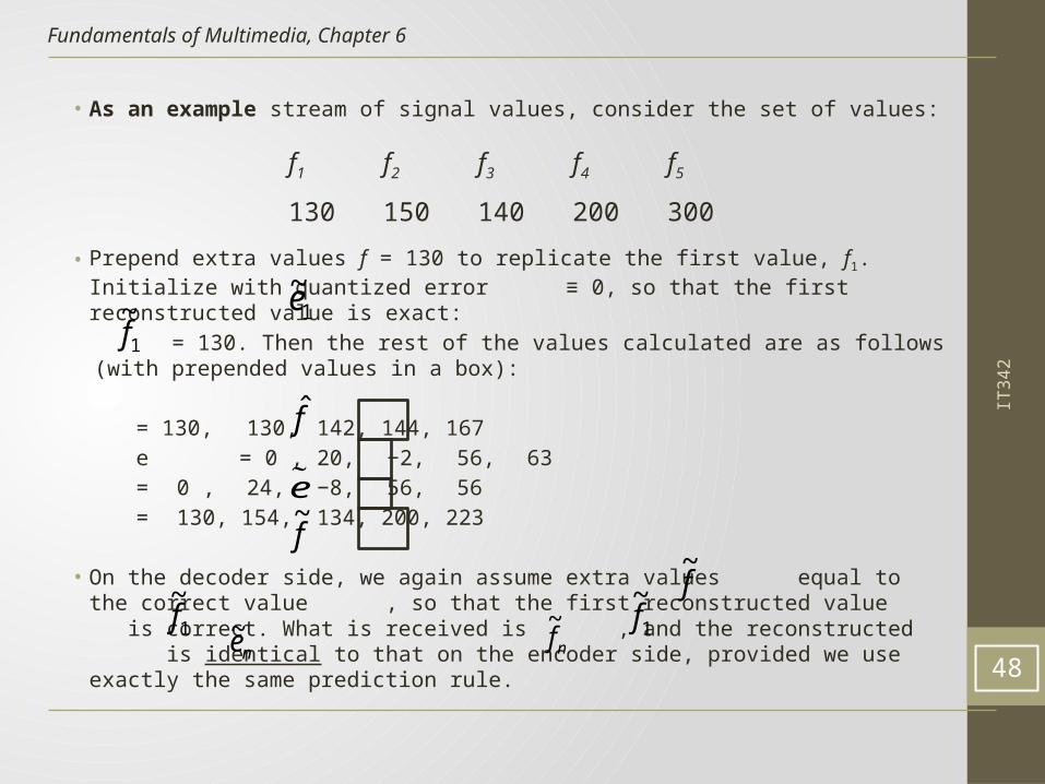
• As an example stream of signal values, consider the set of values:

• Prepend extra values f = 130 to replicate the first value, f1. Initialize with quantized error ≡ 0, so that the first reconstructed value is exact: = 130. Then the rest of the values calculated are as follows (with prepended values in a box):

= 130, 130, 142, 144, 167 e = 0 , 20, −2, 56, 63

= 0 , 24, −8, 56, 56 = 130, 154, 134, 200, 223

• On the decoder side, we again assume extra values equal to the correct value , so that the first reconstructed value is correct. What is received is , and the reconstructed is identical to that on the encoder side, provided we use exactly the same prediction rule.

48

f1 f2 f3 f4 f5

130 150 140 200 300

e

1~e

1

~f

f̂

f~

f~

1

~f 1

~f

ne~ nf~

IT34

2


DM• DM (Delta Modulation): simplified version of DPCM. Often used

as a quick AD converter.1. Uniform-Delta DM: use only a single quantized error value,

either positive or negative.a) a 1-bit coder. Produces coded output that follows the original signal

in a staircase fashion. The set of equations is:

Note that the prediction simply involves a delay.49

1

1

ˆ ,

ˆ ,

if 0,

ˆ .

n n

n n n n n

nn

n n n

f f

e f f f f

k e where k is a constante

k otherwise

f f e

IT34

2


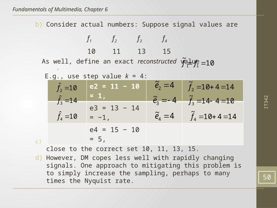
b) Consider actual numbers: Suppose signal values are

As well, define an exact reconstructed value . E.g., use step value k = 4:

c) The reconstructed set of values 10, 14, 10, 14 is close to the correct set 10, 11, 13, 15.

d) However, DM copes less well with rapidly changing signals. One approach to mitigating this problem is to simply increase the sampling, perhaps to many times the Nyquist rate.

50

f1 f2 f3 f4

10 11 13 15

e2 = 11 − 10 = 1,

e3 = 13 − 14 = −1,

e4 = 15 − 10 = 5,

10~

11 ff

102̂ f

143̂ f

104̂ f

4~2 e

4~3 e

4~4 e

14410~

2 f

10414~

3 f

14410~

4 f

IT34

2


2. Adaptive DM: If the slope of the actual signal curve is high, the staircase approximation cannot keep up. For a steep curve, should change the step size k adaptively.• One scheme for analytically determining the best set of quantizer

steps, for a non-uniform quantizer, is Lloyd-Max.

51

IT34

2


ADPCM• ADPCM (Adaptive DPCM) takes the idea of adapting the coder

to suit the input much farther. The two pieces that make up a DPCM coder: the quantizer and the predictor.1. In Adaptive DM, adapt the quantizer step size to suit the input.

In DPCM, we can change the step size as well as decision boundaries, using a non-uniform quantizer. We can carry this out in two ways:

(a) Forward adaptive quantization: use the properties of the input signal.

(b) Backward adaptive quantizationor: use the properties of the quantized output. If quantized errors become too large, we should change the non-uniform quantizer.

52

IT34

2


2. We can also adapt the predictor, again using forward or backward adaptation. Making the predictor coefficients adaptive is called Adaptive Predictive Coding (APC):

(a) Recall that the predictor is usually taken to be a linear function of previous reconstructed quantized values, .

(b) The number of previous values used is called the “order” of the predictor. For example, if we use M previous values, we need M coefficients ai, i = 1..M in a predictor

(6.22)

53

1

ˆM

n i n ii

f a f

nf~

IT34

2


• However we can get into a difficult situation if we try to change the prediction coefficients, that multiply previous quantized values, because that makes a complicated set of equations to solve for these coefficients:• Suppose we decide to use a least-squares approach to solving a

minimization trying to find the best values of the ai:

(6.23)

• Here we would sum over a large number of samples fn, for the current patch of speech, say. But because depends on the quantization we have a difficult problem to solve. As well, we should really be changing the fineness of the quantization at the same time, to suit the signal’s changing nature; this makes things problematical.

54

2

1

ˆ( )N

n nn

min f f

nf̂

IT34

2


• Instead, one usually resorts to solving the simpler problem that results from using not in the prediction, but instead simply the signal fn itself. Explicitly writing in terms of the coefficients ai, we wish to solve:

(6.24)

• Differentiation with respect to each of the ai, and setting to zero, produces a linear system of M equations that is easy to solve. (The set of equations is called the Wiener-Hopf equations.)

55

2

1 1

( )N M

n i n in i

min f a f

nf~

IT34

2


• Fig. 6.18 shows a schematic diagram for the ADPCM coder and decoder:

• Fig. 6.18: Schematic diagram for ADPCM encoder and decoder

56

Documents

Chapter 6 Basics of Digital Audio 6.1 Digitization of Sound 6.3 Quantization and Transmission of Audio 1 IT342