Chapter 5 Velocities of H and metal lines in the roAp star ...ikb/thesis/baldry-ch5.pdf · and metal lines in the roAp star Circini ... 1996 May 12 La Silla 3.98 156 215.77 ... 56

Chapter 5

Velocities of H� and metal lines in theroAp star � Circini

The content of this chapter was published in paper Baldry et al. (1998b) in collaborationwith Tim Bedding, Michael Viskum, Hans Kjeldsen and Soren Frandsen. I wrote thepaper and reduced the data, with the exception that M. Viskum reduced the La Silladatafrom the CCD images to the 1D spectra. I observed at Mt. Stromlo while M. Viskumobserved at La Silla. M. Viskum and I were supervised by the other collaborators.

51

52 Chapter 5. Velocities of H� and metal lines in� Circini

5.1 Introduction

Rapidly oscillating Ap (roAp) stars are a sub-class of the chemically peculiar magnetic(Ap or CP2) stars. The Ap phenomenon is characterised by spectra with anomalouslystrong lines of Si, Sr, Cr, other iron peak elements, Eu and other rare earthelements.The stars also have strong global magnetic fields of typically a few kG. The causeofthe abundance anomalies is thought to be magnetically guided chemical diffusion, madepossible because Ap stars have slower rotation rates than normal A stars.Some Ap starsalso show evidence of an inhomogeneous distribution of elements (in spots) on the surfaceof the star (Rice & Wehlau 1991). Despite the name, the Ap stars range in temperaturefrom spectral type B8 to F0 (luminosity class IV-V). At the cool-end of the range, the Apstars overlap the instability strip and this is where the roAp stars are found. However, notall the Ap stars in the instability strip have been observed to pulsate (Mathys et al. 1996).A review of roAp stars with a comprehensive list of references is given by Kurtz (1990).Later reviews are given by Matthews (1991, 1997, 1998) and Martinez & Kurtz (1995a,1995b), and a review on the theoretical aspects is given by Shibahashi (1991).

About thirty percent of main-sequence (normal) A-stars in the instability strip pulsatewith photometric amplitudes greater than 10 mmag and with periods in the range 30–360minutes; these are� Scuti stars. However, the roAp stars are characterised by photometricamplitudes below 8 mmag and periods in the range 5–15 minutes. Both� Scuti and roApstars pulsate in low-degree (` �3) p-modes but while the� Scuti stars pulsate with low-overtones, the roAp stars vibrate in very high-overtones (n�25–50). Explaining why thechemically peculiar roAp stars pulsate in much higher overtones than the normal � Scutistars remains one of the exciting challenges in this field. For recent theoretical work ondifferent aspects of roAp stars, see Takata & Shibahashi (1995); Dziembowski &Goode(1996); Audard et al. (1998); Gautschy et al. (1998).

5.1.1 � Cir� Circini (HR 5463, HD 128898, V=3.2, spectral type Ap SrEu(Cr) ) is the brightest of theknown roAp stars. It is situated at a distance of16:4�0:2 pc (parallax61:0�0:6mas, HIP71908, Perryman et al. 1997) and is a visual binary (secondary, V=8.2) with a separationof 15.6 arcsec. Kurtz & Martinez (1993) determined an equivalent spectral type of A6V(Te� = 8000K), while Kupka et al. (1996) have derivedTe� = 7900� 200 K and logg =4:2� 0:15.

Previous observations of this star in photometry (Kurtz et al. 1994b) have shown thatits principal pulsation mode is a pure oblique dipole mode (`=1) with a frequency of2442�Hz (P = 6:825 min). Kurtz et al. (1994b) measured the amplitude of the principalmode to be2:55mmag (Stromgrenv). They also found two rotationally split side-lobes(�0:27mmag), four weaker modes (�0:15mmag) and the first harmonic of the principalmode (� 0:20mmag). It has also been observed that the photometric amplitude dependson the wavelength (Weiss et al. 1991, Medupe & Kurtz 1998), with amplitude decreas-ing with increasing wavelength. In Section 5.5.3 we relate these wavelength dependentphotometric amplitudes to our results.

5.2. Observations 53

The vast majority of studies of roAp stars have been made using photometry. In threestars, HR 1217 (Matthews et al. 1988), Equ (HR 8097; Libbrecht 1988, Kanaan &Hatzes 1998) and 10 Aql (HR 7167; Chagnon & Matthews 1998), oscillations have beenconvincingly detected in Doppler shift. For� Cir, based on the photometric amplitudegiven above, the relation of Kjeldsen & Bedding (1995) predicts a velocity amplitudeof 160 m s�1. Belmonte et al. (1989) claimed a detection in� Cir at an amplitude of1000 m s�1 using a line at 5317.4A, but this result was in doubt given that Schneider &Weiss (1989) had set an upper limit of 100 m s�1 for possible radial velocity variations,using a wavelength region from 6450A to 6500A. More recently, an upper limit for� Cirof only 36 m s�1 (peak-to-peak) was set by Hatzes & Kurster (1994) at the frequencyof the principal photometric pulsation mode, using a wavelength region from 5365A to5410A. In this chapter we examine the radial velocity amplitude of the principal mode fordifferent wavelength bands. From our work (see also Viskum et al. 1998a) and from thework by Kanaan & Hatzes (1998) on Equ, it is apparent that the velocity amplitude inroAp stars can vary significantly from line to line, and that previous upper limits reflectaverages over the wavelength regions used.

5.2 Observations

We have obtained intermediate-resolution spectra of� Cir using the coude spectrograph(B grating) on the 74-inch (1.88-m) Telescope at Mt. Stromlo, Australia and the DFOSCspectrograph mounted on the Danish 1.54m at La Silla, Chile. We have a total of 6366spectra from a period of 2 weeks in 1996 May (Table 5.1).

The Stromlo data consist of single-order spectra, projected onto a 2K Tektronix CCD,with a wavelength coverage of 6000A to 7000A. The dispersion was 0.49A/pixel andwas nearly constant across the spectrum, with a resolution of approximately 1.5A set bythe slit width of 2 arcsec. The typical exposure time was 28 seconds, with an over-headbetween exposures of 17 seconds. The average number of photons/A in each spectrumwas about 800 000.

The La Silla data consist of echelle spectra containing six orders, projectedonto a 2KLORAL CCD, with a total wavelength coverage of 4500A to 8000A. For this chapter, wehave only considered the order containing H�, which covers the range 6200A to 7200A.The dispersion varied from 0.51A/pixel to 0.70A/pixel across this order, giving a similarresolution to the Stromlo data. For the La Silla data, the typical exposure timewas 40seconds with an over-head of 42 seconds. The average number of photons/A in the H�order of each spectrum ranged from about 480 000 at the blaze peak (6700A) to about120 000 at the blue end (6200A).


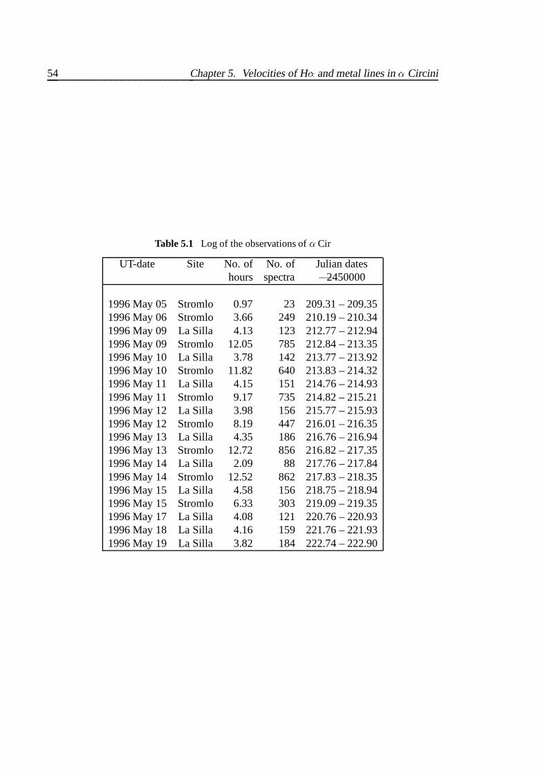
Table 5.1 Log of the observations of� Cir

UT-date Site No. of No. of Julian dateshours spectra �2450000

1996 May 05 Stromlo 0.97 23 209.31 – 209.351996 May 06 Stromlo 3.66 249 210.19 – 210.341996 May 09 La Silla 4.13 123 212.77 – 212.941996 May 09 Stromlo 12.05 785 212.84 – 213.351996 May 10 La Silla 3.78 142 213.77 – 213.921996 May 10 Stromlo 11.82 640 213.83 – 214.321996 May 11 La Silla 4.15 151 214.76 – 214.931996 May 11 Stromlo 9.17 735 214.82 – 215.211996 May 12 La Silla 3.98 156 215.77 – 215.931996 May 12 Stromlo 8.19 447 216.01 – 216.351996 May 13 La Silla 4.35 186 216.76 – 216.941996 May 13 Stromlo 12.72 856 216.82 – 217.351996 May 14 La Silla 2.09 88 217.76 – 217.841996 May 14 Stromlo 12.52 862 217.83 – 218.351996 May 15 La Silla 4.58 156 218.75 – 218.941996 May 15 Stromlo 6.33 303 219.09 – 219.351996 May 17 La Silla 4.08 121 220.76 – 220.931996 May 18 La Silla 4.16 159 221.76 – 221.931996 May 19 La Silla 3.82 184 222.74 – 222.90

5.3. Reductions 55

Figure 5.1 Template spectrum of� Cir from the Stromlo data set

5.3 Reductions

5.3.1 Extraction of spectra

IRAF procedures were used to reduce the data from 2D images to 1D spectra. Theseinvolved bias subtraction, flat-field division, and extraction of the orders including back-ground scattered-light subtraction. Additionally the Stromlo data were corrected for non-linearities on the CCD image after bias subtraction (Chapter 3). This was necessary be-cause the ratio between expected-counts and measured-counts varied by 7% from low-light levels to digital saturation. After correction, the data were linearto within 1%. TheLa Silla data were measured to be linear within 0.5%.

After reduction to the 1D stage, the spectra were fitted using the IRAF procedure,continuum, in which low points are excluded until a fit is obtained close to the contin-uum level. A third order polynomial fit was used for the Stromlo data and a second orderfit for the La Silla data. For each data set, a template spectrum was obtained by averaging25 high-quality spectra (Figure 5.1 or; for a close-up: Figures A.1–A.2).

5.3.2 Cross-correlations

The spectra obtained from Mt. Stromlo were divided into 89 unequal wavelength bands(Table 5.3). Except for the region containing H�, the bands were non-overlapping andtypically contained a few lines. The boundaries were chosen at places where twoor threepixels were nearly at the same level (close to the continuum). In the case ofH�, wedefined four bands of different widths, each centred on the core (band nos. 85–88). Only66 of these bands were used from the La Silla spectra because of the different wavelengthcoverage.

A cross-correlation technique was applied to measure the Doppler shift of eachband


in each spectrum, relative to the same band in the template spectrum. Thefollowingprocedure was applied:

(i) a linear local continuum fit was applied across the band using the edge pixels;

(ii) the spectral band was linearly rebinned by a factor of 40 and 1.0 was subtractedsuch that the edge pixels were nearly zero;

(iii) a half-cosine filter was applied across 3 pixels at the edges so that there was asmooth transition between zero outside the band and nearly zero on the edge pixels;

(iv) the spectral band was cross-correlated (using Fast Fourier Transforms) with theband from the template spectrum, which had been processed in the same way;

(v) the peak of the cross-correlation function was found by fitting a quadratic to 9 pointsaround the peak point.

With this procedure, we could measure shifts to within 0.02 pixels (400 m s�1) in most ofthe spectra.

5.3.3 Velocity reference

The dominant cause of scatter in the velocity measurements is the global shiftsof the lighton the spectrograph. To correct for this, we have used the strong telluric O2 absorptionband around 6870A as a velocity reference (band no. 80). The noise factors associatedwith using a telluric reference are the instability of the telluric atmospheric band andthe changes in dispersion of the spectrograph, which affects the relative shiftbetween atarget band and the reference band. In our data, the variance of the noise when usingthe telluric reference was about one-tenth of the variance when using no reference, whenmeasuring a target band about 300A away from the telluric reference. Note that we wereonly interested in high-frequencies (periods less than 15 minutes) for this analysis, so thatslow drifts of the spectrograph and an absolute measure of the radial velocity ofthe starwere not important.

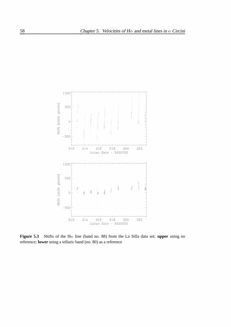
Figures 5.2–5.3 show the Stromlo and La Silla H� velocity time-series, with the im-provement in noise level that is made when a telluric band is used as a velocity reference.

This is particularly evident for the H� Doppler shift, for which the noise is dominatedby instrumental factors rather than photon-noise.

5.3.4 Time-series analysis

The time-series for the 88 different bands (not including the velocity reference) werehigh-pass filtered, and then cleaned for bad data points by removing any points lyingoutside�6:5 times the median deviation. Next, a weighted least-squares fitting routinewas applied to each time series (using heliocentric time) to produce amplitude spectra.

5.3. Reductions 57

Figure 5.2 Shifts of the H� line (band no. 88) from the Stromlo data set;upper using noreference;lower using a telluric band (no. 80) as a reference. Note that thereare larger noiselevels in the data at the beginning and end of each night. These points received lower weight inthe time-series analysis.


Figure 5.3 Shifts of the H� line (band no. 88) from the La Silla data set;upper using noreference;lower using a telluric band (no. 80) as a reference

5.4. Results on the principal mode 59

Figure 5.4 Amplitude spectrum for wavelength band no. 18, using the Stromlo data set. Thisfigure clearly shows a peak at the principal frequency (2442�Hz), and shows the regions whichwere used to calculate the noise-level (1100–2300�Hz and 2600–4400�Hz). The side lobes to themain peak are caused by aliasing. The signal-to-noise ratioof the principal peak in this spectrumis 11.5.

5.4 Results on the principal mode

We have concentrated on using the Stromlo data for comparison between the differentbands. This is because the La Silla data only covers bands 23–88 and also has a highernoise level per spectrum for the cross-correlation measurements. Also, weare only ex-amining the principal pulsation mode with individual bands, therefore there is no need touse the dual-site combined data to reduce aliasing. This allows us to use the La Silla datato check the results obtained using the Stromlo data (Section 5.4.2).

Figure 5.4 shows the amplitude spectrum of a band with a strong peak at the principalphotometric frequency, and Figures 5.5–5.6 show that the principal mode is evident evenwith quite low signal-to-noise ratios (4.4 and 3.1).

We measured the frequency of the principal mode to be 2442.05�0.02�Hz using theStromlo data set, and 2442.02�0.03�Hz using the combined data from both sites. Thisis in agreement with photometric frequencies measured in the same time period by DonKurtz (private comm., see Table 5.2) as part of an ongoing project of measuring frequencychanges in roAp stars (Section 6 from Martinez & Kurtz 1995b, Kurtz et al. 1997). Thetwo calculations from the photometric data, shown in Table 5.2, are over 130 days and 31days. We have set our phase reference-point (t0) to coincide with maximum light, usingthe first calculation. Our velocity phases are measured at this reference-point, with theconvention that a phase of 0� represents maximum velocity (red-shift). For example, aphase of�30� means that the velocity curve lags behind the light curve by 30�. Note thatthe second calculation indicates that there may have been some frequency changesduringthe time period of the first. If this is the case, then maximum light may not coincide with


Figure 5.5 Amplitude spectrum for wavelength band no. 57. The signal-to-noise ratio in thisspectrum is 4.4.

Figure 5.6 Amplitude spectrum for wavelength band no. 44. The signal-to-noise ratio in thisspectrum is 3.1.

Table 5.2 Photometric amplitudes (JohnsonB) and frequencies, of the principal mode, mea-sured by Don Kurtz (private comm.). The reference-point (t0) for the phase measurements is JD2450215.07527, with the convention that a phase of 0� represents maximum light.

Julian dates frequency amplitude phase�2450000 (�Hz) (mmag) (degrees)

142 – 272 2442.039�0.002 1.74�0.07 0.0�2.4213 – 244 2442.022�0.011 1.63�0.12 15.3�7.3


Figure 5.7 Amplitudes and phases of the principal pulsation mode in� Cir for different wave-length bands, using the Stromlo data. Only the bands with a signal-to-noise ratio greater than 3.0are plotted. The diamonds represent three different wavelength bands across the H� line, and thesquares represent bands that contain some telluric lines. Note that the data are plotted twice forclarity.

the reference-point by up to�20� of a cycle.We have measured the amplitude and phase of each time-series at 2442.03�Hz and

estimated the rms-noise level by averaging over surrounding frequencies (1100–2300�Hzand 2600–4400�Hz). See Figure 5.4 for an example. The results are shown in Table 5.3.

5.4.1 Amplitude and phase variations

The amplitude and phase of the principal photometric mode vary significantly betweendifferent bands, with some bands that are pulsating in anti-phase with others. Figure 5.7shows an amplitude vs. phase diagram for bands for which the signal-to-noise ratio inthe amplitude spectrum is greater than 3.0. For these bands we can be sure that we havedetected the principal pulsation and that the phase is reasonably well defined. For the un-certainty in the amplitude, we have used the rms-noise level directly. Forthe uncertainty


Table 5.3 Information on wavelength bands from� Cir showing amplitude and phase at2442.03�Hz (from the Stromlo data set) – Part A

band wavelengths EWa ampl. noiseb S/N phasec errord noteseno. (A) (A) (m s�1) (m s�1) (deg.) (deg.) on lines

00 6011.3 – 6018.2 0.143 136 60 2.2 171 26 Mn I01 6019.1 – 6036.4 0.205 55 49 1.1 51 62 Fe I, Mn I, Si I02 6037.7 – 6047.1 0.066 227 88 2.6 105 23 S I, Ce II, Fe II03 6048.5 – 6050.6 0.017 56 72 0.8 — — Eu II, Co I04 6051.9 – 6058.9 0.111 207 45 4.6 257 13 Cr II, Fe I, S I05 6060.2 – 6073.6 0.083 93 52 1.8 24 34 Fe I, Cr II, Co I06 6074.9 – 6084.8 0.074 189 49 3.8 2 15 Fe I, Co I, Fe II07 6086.2 – 6095.6 0.108 411 45 9.1 208 6 Cr II, Co I, Si I08 6099.4 – 6109.3 0.183 46 33 1.4 9 45 Ca I, Fe I09 6110.7 – 6118.1 0.042 405 90 4.5 198 13 Fe II, Si I, Cr II, Co I10 6120.5 – 6126.9 0.145 49 32 1.5 12 41 Ca I, Si I11 6127.8 – 6133.8 0.054 71 63 1.1 70 62 Si I, Cr II, Fe I12 6135.2 – 6139.7 0.134 11 39 0.3 — — Fe I13 6141.0 – 6151.4 0.262 157 31 5.1 274 11 Fe II, Si I, Ba II14 6153.3 – 6164.6 0.383 178 31 5.7 7 10 Ca I, Si I15 6166.0 – 6171.5 0.133 60 30 2.0 140 30 Ca I, Fe I16 6172.9 – 6181.8 0.046 26 65 0.4 — — Cr II, Fe II, Eu II17 6184.1 – 6193.0 0.018 45 42 1.1 321 70 Fe I18 6194.4 – 6197.5 0.055 507 44 11.5 202 5 Cr II, Si I19 6198.8 – 6210.2 0.033 195 98 2.0 45 30 Ca II, Cr II, Fe I20 6212.5 – 6217.5 0.055 140 82 1.7 243 36 Ti II, Fe I21 6218.4 – 6223.4 0.048 394 86 4.6 352 13 Fe I, Ti II22 6224.8 – 6228.3 0.016 64 125 0.5 — — Cr II, Fe I, V II23 6229.2 – 6234.7 0.101 26 45 0.6 — — Fe I, Co I24 6236.0 – 6241.5 0.159 105 41 2.6 336 23 Fe II, Si I25 6242.9 – 6250.3 0.234 84 34 2.5 53 24 Si I, Fe II, Fe I26 6251.7 – 6263.1 0.138 89 45 2.0 293 31 Fe I, Si I27 6264.4 – 6274.8 0.045 226 77 2.9 341 20 Co I, Fe I28 6275.7 – 6287.1 0.478 160 28 5.7 357 10 telluric, Co I29 6288.9 – 6296.9 0.099 114 39 2.9 36 20 telluric, Fe I30 6297.7 – 6308.1 0.202 68 29 2.4 308 25 Fe I, telluric31 6309.0 – 6312.5 0.051 130 51 2.6 334 23 telluric, Si I32 6313.4 – 6325.3 0.308 130 36 3.6 125 16 Ca I, Fe II, Fe I33 6326.1 – 6333.6 0.106 460 38 12.2 260 5 Sm II(?), Fe II, Si I34 6335.0 – 6338.5 0.048 119 56 2.1 17 28 Fe I, Cr II35 6340.8 – 6350.7 0.319 89 26 3.4 7 17 Si II, Ca I36 6352.1 – 6367.4 0.266 184 39 4.7 353 12 Ca I37 6368.3 – 6373.7 0.143 35 29 1.2 287 55 Si II38 6375.1 – 6387.9 0.090 440 66 6.7 306 9 Fe II, Fe I39 6389.3 – 6397.2 0.077 100 49 2.0 297 30 Fe I40 6398.6 – 6402.1 0.066 86 38 2.3 20 26 Fe I41 6404.5 – 6412.9 0.132 78 30 2.5 14 23 Fe I42 6414.3 – 6423.2 0.210 245 33 7.4 298 8 Fe II, Fe I, Co IaApproximate total equivalent-width of lines in band, relative to local fit across band.brms-noise estimated from amplitude spectrum using 1100–2300�Hz and 2600–4400�Hz.cPhase is calculated with respect to a reference-point (t0) at JD 2450215.07527, and the convention is that a phase of 0� represents

maximum velocity (red-shift).dError in the phase is taken to be arcsin (rms-noise/amplitude).eNotes on each band giving the probable dominating absorption lines derived from synthetic spectra supplied by Friedrich Kupka(private comm.).


Table 5.4 Information on wavelength bands from� Cir showing amplitude and phase at2442.03�Hz (from the Stromlo data set) – Part B

band wavelengths EWa ampl. noiseb S/N phasec errord noteseno. (A) (A) (ms�1) (ms�1) (deg.) (deg.) on lines

43 6424.6 – 6435.4 0.152 69 47 1.5 332 43 Fe II, Fe I44 6436.8 – 6441.3 0.132 86 28 3.1 79 19 Ca I, Eu II45 6442.2 – 6444.7 0.013 120 95 1.3 100 52 Si I, Fe II, Co I46 6448.1 – 6452.6 0.146 39 26 1.5 83 42 Ca I, Co I47 6453.5 – 6460.4 0.363 70 20 3.5 22 17 Fe II, Ca II48 6461.8 – 6465.3 0.100 93 24 3.9 13 15 Ca I49 6468.1 – 6478.0 0.218 29 30 1.0 — — telluric, Ca I50 6478.9 – 6488.3 0.152 114 38 3.0 236 19 telluric, Fe II51 6489.7 – 6501.5 0.422 69 33 2.1 229 28 Ca I, Fe I, Ti II, Ba II52 6502.4 – 6509.9 0.012 88 84 1.0 174 73 telluric, Fe I53 6511.2 – 6521.1 0.395 49 23 2.1 20 29 Fe II, telluric54 6522.5 – 6529.0 0.110 311 37 8.4 327 7 telluric, Si I55 6530.3 – 6538.8 0.078 86 60 1.4 6 45 telluric, S I

56 6585.2 – 6589.7 0.055 25 88 0.3 — — Fe II, C I57 6591.1 – 6596.5 0.049 294 67 4.4 207 13 Fe I58 6597.9 – 6607.3 0.015 989 90 11.0 16 5 Sm II(?), Ti II59 6608.7 – 6620.0 0.047 156 56 2.8 293 21 Y II, Co I, Fe I60 6623.9 – 6640.6 0.100 296 69 4.3 64 13 Fe I, Si I, Co I61 6642.0 – 6652.9 0.066 259 50 5.2 334 11 Eu II62 6654.2 – 6658.7 0.021 139 189 0.7 — — C I, Ca I63 6660.1 – 6674.9 0.084 199 67 3.0 351 20 Fe I, Cr I, Si I64 6676.3 – 6682.2 0.100 517 54 9.6 181 6 Fe I, Ti II65 6683.1 – 6714.1 0.042 267 63 4.3 304 14 Al I, Fe I, Ca I66 6715.4 – 6719.5 0.062 56 38 1.5 302 43 Ca I67 6720.8 – 6724.3 0.030 147 69 2.1 213 28 Si I68 6725.2 – 6746.4 0.040 519 96 5.4 5 11 S I, Fe I69 6747.3 – 6754.2 0.044 214 107 2.0 324 30 S I, Fe I, Si I70 6755.6 – 6759.1 0.031 139 78 1.8 272 34 S I71 6760.5 – 6779.2 0.013 95 112 0.8 — — Co I, Si I, Ni I72 6781.5 – 6788.0 0.030 798 146 5.5 28 11 Ti II73 6788.9 – 6798.3 0.067 490 80 6.1 33 9 Y II74 6800.6 – 6823.8 0.021 344 81 4.3 338 14 Co I, Fe I, Si I75 6826.6 – 6830.1 0.042 171 58 3.0 258 20 Ti II, C I, Fe I76 6831.5 – 6834.5 0.013 177 149 1.2 59 58 Y II77 6835.9 – 6850.2 0.153 78 88 0.9 — — Fe I78 6851.6 – 6859.0 0.065 64 56 1.1 138 61 Fe I, Si I79 6860.4 – 6863.9 0.018 494 114 4.3 1 13 Si I, Fe I, Fe II80 6864.8 – 6881.0 3.605 telluric reference81 6881.9 – 6902.1 1.958 36 14 2.5 318 23 telluric82 6903.0 – 6920.2 0.832 30 10 3.0 263 19 telluric83 6921.6 – 6966.2 2.424 42 12 3.5 358 16 telluric84 6968.6 – 7007.4 1.184 45 21 2.2 322 27 telluric

85 6522.0 – 6607.8 10.398 168 13 13.1 325 4 H�86 6538.2 – 6590.2 7.774 174 12 14.1 332 4 H�87 6545.5 – 6578.4 5.486 166 12 13.7 324 4 H�88 6554.3 – 6571.1 2.931 182 12 14.9 328 4 H�1;2;3;4;5See Table 5.3.


Figure 5.8 Histogram of the data in Figure 5.7 in phase bins of 30�. In total, 33 bands are plotted,with only one band across H� included.

in the phase, we have used simple complex arithmetic to find the maximum change inphase that a rms-noise vector could induce i.e. arcsin (rms-noise/amplitude).

Figure 5.8 shows a histogram of the phases of the principal mode. Most bands havephases that lie between�60� and 30� but there is also a group of five bands with phasesbetween 180� and 210�. We suggest that these two groups might be associated with twosections of the atmosphere either side of a pulsational node (zero-point). However,thereis more variation in the phases than can be accounted for purely by using a standingwave model. Perhaps there is also a travelling component to the pulsational wave inthe star’s atmosphere. Another possibility is that we are seeing asymmetric temperature(equivalent-width) changes that create apparent Doppler shifts and therefore produce avariety of phases. For example, consider two lines at different wavelengths which areblended. If a temperature change causes the relative strength of the two lines to changethen a pseudo-Doppler shift may be measured from the blended profile.

The line identification for the different bands (Table 5.3) is only an approximate anal-ysis based on synthetic spectra (Friedrich Kupka, private comm.) using recently derivedabundances (Kupka et al. 1996). Nearly all the bands that we have measured are com-posed of blended lines in our spectra. Therefore it has been difficult to determineif thereis a pattern associating the line-type with the measured amplitude of the pulsation. Onenoticeable pattern is that the largest amplitudes occur only in the weaker lines, this is seenfrom a plot of amplitude vs. total equivalent width of the band (Figure 5.9). Possibly thisis because weaker lines are more likely to be formed in a narrower sectionof the star’satmosphere and therefore phase smearing between different parts of a pulsationwave isminimised. Kanaan & Hatzes (1998) have also found that the velocity amplitude tends tobe higher (up to 1000 m s�1) in the weaker lines of the roAp star Equ.


Figure 5.9 Amplitude of the principal pulsation mode as a function of total equivalent-width forbands 0–79, using the Stromlo data. The squares represent bands that contain some telluric lines.

5.4.2 Comparing the data sets

The amplitude vs. phase diagram for the La Silla data is shown in Figure 5.10. Theamplitudes and phases measured from the two data sets are in complete agreement, atthe 2� level, with the exception of bands 58 and 79. These have larger amplitudes whenmeasured using the La Silla data (Table 5.5). Amplitude variation is not unexpected sincethe photometric amplitude varies as a function of rotation phase of the star (rotation period4.48 days, Kurtz et al. 1994b). The La Silla time-series may sample the rotational phasesof the star in such a way to produce a larger amplitude on average. Other possible reasonsare that the bands are not exactly equal for the two data sets (they are slightly outofalignment by about 0.5 to 1 pixel) and that the dispersions are different (see Section 5.2).

Table 5.5 Comparison of the large velocity amplitude bands between the Stromlo and the LaSilla data sets

Band no. Stromlo measurement La Silla measurement

58 990� 90 m s�1 1660�280 m s�172 800�150 m s�1 960�400 m s�179 490�110 m s�1 1370�380 m s�1


Figure 5.10 Amplitudes and phases of the principal pulsation mode for different bands, using theLa Silla data (which covers bands 23–88). This figure is similar to Figure 5.7 except, additionallythe bands with a signal-to-noise ratio between 2.0 and 3.0 are plotted (with dotted lines). Alsonote that the amplitude scale extends to 2000m s�1 rather than 1100 m s�1.

5.5. Discussion and conclusions 67

5.5 Discussion and conclusions

5.5.1 Techniques

We have shown that it is possible to obtain high-precision velocity measurements withmedium-dispersion spectrographs using telluric lines as a reference. For the Dopplershift of the H� line, we have obtained a noise level of 500 m s�1 per spectrum from Mt.Stromlo and 900 m s�1 per spectrum from La Silla. These measurement are not limitedby photon-noise, so the difference in precision between the two sites must be due toeitherthe instrument (coude vs. Cassegrain) or the telluric reference. Given that Mt. Stromlo(750m) is situated at a lower altitude than La Silla (2400m), we note that a possibleadvantage of low altitude sites is that the telluric lines are more stable.This is plausiblesince the lines will be stronger, and temperature and velocity changes will be averagedover a longer distance in the Earth’s atmosphere.

We chose the strongest telluric feature (band 80) as our velocity reference. Thetotalequivalent-width (EW) of the metal lines within this band was estimated (using the syn-thetic spectra) to be approximately 2 percent of the total EW of the band. Other bands(81–84), which are also dominated by telluric lines, show low-amplitude oscillation sig-nals with signal-to-noise ratios from 2.2 to 3.5. This is not surprising since these bandshave about 6%, 12%, 9% and 23% of their total EW coming from metal lines.

5.5.2 Velocity amplitudes

Schneider & Weiss (1989) set an upper limit of 100 m s�1 for radial velocity variations in� Cir but this was set assuming no amplitude and phase differences between lines. Fromtheir Table 4, it can be seen that only from lines at 6462.6A and 6494.99A can amplitudesabove 100 m s�1 be ruled out. This is in agreement with our measured amplitudes in bands48 and 51 which are 93�24 m s�1 and 69�33 m s�1 respectively.

We cannot compare our results directly with the upper limit of only 18 m s�1 set byHatzes & Kurster (1994), but our results show that such a low limit could be setif therewere only lines with low amplitude, and perhaps different phases, in the region used bythem (5365–5410A). Kanaan & Hatzes (1998) have measured radial velocity variationsin Equ in a similar wavelength region (5373–5394A) and find an average amplitudeof 30 m s�1. In conclusion, our measured amplitude differences between bands are con-sistent with previous upper limits on velocity variations in� Cir and are comparable tothe amplitude differences found in Equ by Kanaan & Hatzes (1998). Furthermore, ourdata lend support to the detection by Belmonte et al. (1989) of a velocity amplitude of1000 m s�1 in � Cir.

5.5.3 Probing the atmosphere

The photometry of roAp stars has revealed a steep decline of pulsational amplitude withincreasing wavelength. Matthews et al. (1990, 1996) have attributed this to the wave-length dependence of limb-darkening. They have determined limb-darkening coefficients


from their amplitude measurements of HR 3831. However, Medupe & Kurtz (1998) sug-gest that limb-darkening is too small an effect to explain the observed decline. Instead,they account for the decline by the change in pulsational temperature amplitude withdepth in the stars,� Cir and HR 3831. This result would imply a surprisingly small ra-dial node separation in the atmosphere of roAp stars (Matthews 1997). The amplitudeand phase variations presented in this chapter (see also Viskum et al. 1998a) suggest thesame, with a radial-node situated in the atmosphere of� Cir. Matthews (1997) suggestedan alternative interpretation, where ions are grouped either side of a horizontalnode onthe surface. Since we can find no simple pattern associating ion type with amplitude orphase, we argue that the phase differences are probably caused by differing formationdepths and therefore there is a radial-node in the atmosphere.

Three bands (Table 5.5) have a particularly large amplitude in one or both data sets.It could be these bands contain elements that are located in spots on the surface ofthestar, near a pole of the dipole pulsation, which is why their velocity amplitude is larger.The argument against this hypothesis is that there is no one element that is a dominatingfactor in all three bands. However, we can not rule out surface inhomogeneities as a factorcontributing to the amplitude and phase variations.

5.5.4 Further work

A time-series of high-resolution spectra would be invaluable in explaining the completerange of amplitudes and phases discovered in� Cir. With our results, we can not rule outsignificant contributions from blending effects to the amplitudes and phases of differentbands. However, with our data set from May 1996 we can look for H� line profile varia-tions. In particular, measuring the width and velocity amplitude at different depths in theH� line (Chapter 6).

Eventually, spectroscopy of� Cir combined with modeling, should be able to map theshape of the pulsation wave in the atmosphere of the star.

Documents

Chapter 5 Velocities of H and metal lines in the roAp star ...ikb/thesis/baldry-ch5.pdf · and metal lines in the roAp star Circini ... 1996 May 12 La Silla 3.98 156 215.77 ... 56