Chapter 5: The Normal Distribution

and the Central Limit Theorem

The Normal distribution is the familiar bell-shaped distribution. It is probablythe most important distribution in statistics, mainly because of its link with theCentral Limit Theorem, which states that any large sum of independent,identically distributed random variables is approximately Normal:

X1 +X2 + . . .+Xn ∼ approx Normalif X1, . . . , Xn are i.i.d. and n is large.

Before studying the Central Limit Theorem, we look at the Normal distributionand some of its general properties.

5.1 The Normal Distribution

The Normal distribution has two parameters, the mean, µ, and the vari-ance, σ2.

µ and σ2 satisfy −∞ < µ <∞, σ2 > 0.

We write X ∼ Normal(µ, σ2), or X ∼ N(µ, σ2).

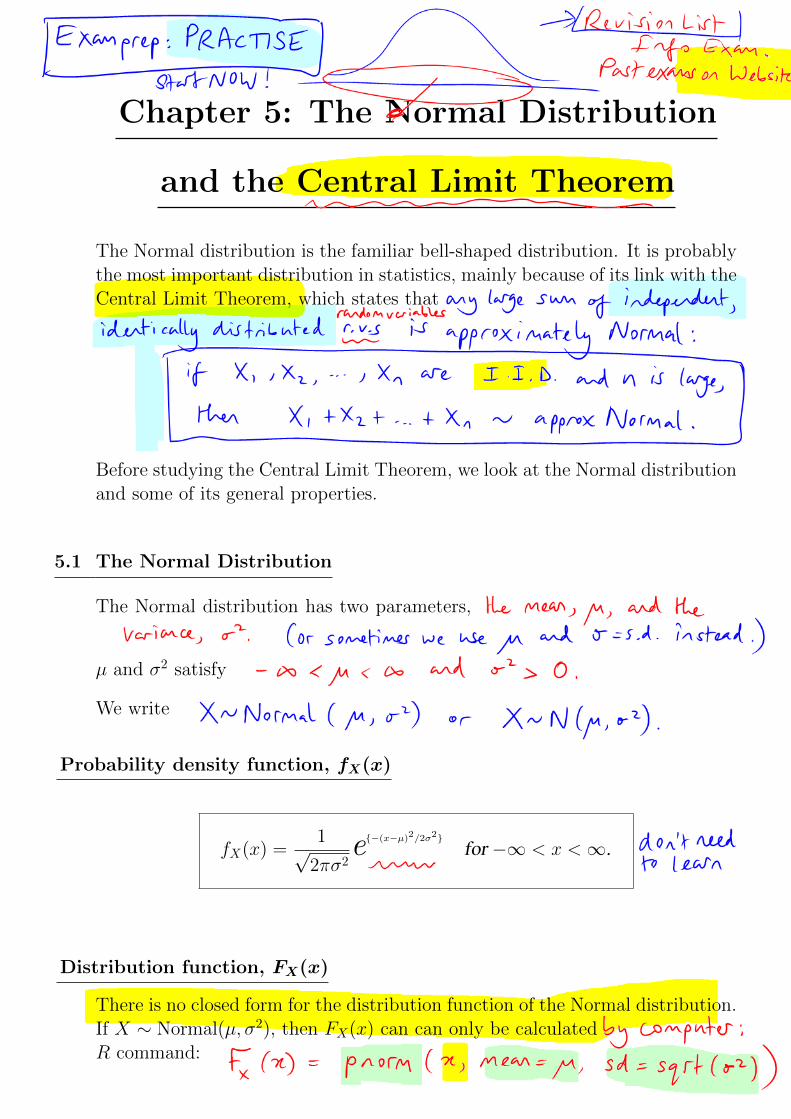
Probability density function, fX(x)

fX(x) =1√

2πσ2e{−(x−µ)

2/2σ2}for −∞ < x <∞.

Distribution function, FX(x)

There is no closed form for the distribution function of the Normal distribution.If X ∼ Normal(µ, σ2), then FX(x) can can only be calculated by computer.R command: FX(x) = pnorm(x, mean=µ, sd=sqrt(σ2)).

165

Probability density function, fX(x)

Distribution function, FX(x)

Mean and Variance

For X ∼ Normal(µ, σ2), E(X) = µ, Var(X) = σ2.

Linear transformations

If X ∼ Normal(µ, σ2), then for any constants a and b,

aX + b ∼ Normal(aµ+ b, a2σ2

).

In particular, put a =1

σand b = −µ

σ, then

X ∼ Normal(µ σ2) ⇒(X − µσ

)∼ Normal(0, 1).

Z ∼ Normal(0, 1) is called the standard Normal random variable.

166

Proof that aX + b ∼ Normal(aµ+ b, a2σ2

):

Let X ∼ Normal(µ, σ2), and let Y = aX + b. We wish to find the distributionof Y . Use the change of variable technique.

1) y(x) = ax+b is monotone, so we can apply the Change of Variable technique.

2) Let y = y(x) = ax+ b for −∞ < x <∞.

3) Then x = x(y) = y−ba for −∞ < y <∞.

4)

∣∣∣∣dx

dy

∣∣∣∣ =

∣∣∣∣1

a

∣∣∣∣ =1

|a| .

5) So fY (y) = fX(x(y))

∣∣∣∣dx

dy

∣∣∣∣ = fX

(y − ba

)1

|a| . (?)

But X ∼ Normal(µ, σ2), so fX(x) =1√

2πσ2e−(x−µ)2/2σ2

Thus fX

(y − ba

)=

1√2πσ2

e−(y−ba −µ)2/2σ2

=1√

2πσ2e−(y−(aµ+b))2/2a2σ2

.

Returning to (?),

fY (y) = fX

(y − ba

)· 1

|a| =1√

2πa2σ2e−(y−(aµ+b))2/2a2σ2

for −∞ < y <∞.

But this is the p.d.f. of a Normal(aµ+ b, a2σ2) random variable.

So, if X ∼ Normal(µ, σ2), then aX + b ∼ Normal(aµ+ b, a2σ2

).

167

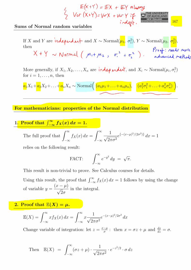
Sums of Normal random variables

If X and Y are independent, and X ∼ Normal(µ1, σ21), Y ∼ Normal(µ2, σ

22),

thenX + Y ∼ Normal

(µ1 + µ2, σ2

1 + σ22

).

More generally, if X1, X2, . . . , Xn are independent, and Xi ∼ Normal(µi, σ2i )

for i = 1, . . . , n, then

a1X1 +a2X2 + . . .+anXn ∼ Normal(

(a1µ1 + . . .+anµn), (a21σ

21 + . . .+a2

nσ2n)).

For mathematicians: properties of the Normal distribution

1. Proof that∫∞−∞ fX(x) dx = 1.

The full proof that

∫ ∞

−∞fX(x) dx =

∫ ∞

−∞

1√2πσ2

e{−(x−µ)2/(2σ2)} dx = 1

relies on the following result:

FACT:

∫ ∞

−∞e−y

2

dy =√π.

This result is non-trivial to prove. See Calculus courses for details.

Using this result, the proof that∫∞−∞ fX(x) dx = 1 follows by using the change

of variable y =(x− µ)√

2σin the integral.

2. Proof that E(X) = µ.

E(X) =

∫ ∞

−∞xfX(x) dx =

∫ ∞

−∞x

1√2πσ2

e−(x−µ)2/2σ2

dx

Change variable of integration: let z = x−µσ : then x = σz + µ and dx

dz = σ.

Then E(X) =

∫ ∞

−∞(σz + µ) · 1√

2πσ2· e−z2/2 · σ dz

168

=

∫ ∞

−∞

σz√2π· e−z2/2 dz

︸ ︷︷ ︸this is an odd function of z(i.e. g(−z) = −g(z)), so itintegrates to 0 over range

−∞ to ∞.

+ µ

∫ ∞

−∞

1√2πe−z

2/2 dz

︸ ︷︷ ︸p.d.f. of N(0, 1) integrates to 1.

Thus E(X) = 0 + µ× 1

= µ.

3. Proof thatVar(X) = σ2.

Var(X) = E{

(X − µ)2}

=

∫ ∞

−∞(x− µ)2 1√

2πσ2e−(x−µ)2/(2σ2) dx

= σ2

∫ ∞

−∞

1√2πz2 e−z

2/2 dz

(putting z =

x− µσ

)

= σ2

{1√2π

[−ze−z2/2

]∞−∞

+

∫ ∞

−∞

1√2πe−z

2/2 dz

}(integration by parts)

= σ2 {0 + 1}

= σ2. �

5.2 The Central Limit Theorem (CLT)

also known as. . . the Piece of Cake Theorem

The Central Limit Theorem (CLT) is one of the most fundamental results instatistics. In its simplest form, it states that if a large number of independentrandom variables are drawn from any distribution, then the distribution of theirsum (or alternatively their sample average) always converges to the Normaldistribution.

169

Theorem (The Central Limit Theorem):

Let X1, . . . , Xn be independent r.v.s with mean µ and variance σ2,from ANY distribution.For example, Xi ∼ Binomial(n, p) for each i, so µ = np and σ2 =np(1− p).

Then the sum Sn = X1 + . . . + Xn =∑n

i=1Xi has a distri-bution that tends to Normal as n→∞.

The mean of the Normal distribution is E(Sn) =∑n

i=1 E(Xi) = nµ.

The variance of the Normal distribution is

Var(Sn) = Var

(n∑

i=1

Xi

)

=n∑

i=1

Var(Xi) because X1, . . . , Xn are independent

= nσ2.

So Sn = X1 +X2 + . . .+Xn → Normal(nµ, nσ2) as n→∞.

Notes:

1. This is a remarkable theorem, because the limit holds for any distributionof X1, . . . , Xn.

2. A sufficient condition on X for the Central Limit Theorem to apply isthat Var(X) is finite. Other versions of the Central Limit Theorem relax theconditions that X1, . . . , Xn are independent and have the same distribution.

3. The speed of convergence of Sn to the Normal distribution depends upon thedistribution of X. Skewed distributions converge more slowly than symmetricNormal-like distributions. It is usually safe to assume that the Central LimitTheorem applies whenever n ≥ 30. It might apply for as little as n = 4.

170

Distribution of the sample mean, X, using the CLT

Let X1, . . . , Xn be independent, identically distributed with mean E(Xi) = µand variance Var(Xi) = σ2 for all i.

The sample mean, X, is defined as:

X =X1 +X2 + . . .+Xn

n.

So X =Snn

, where Sn = X1 + . . . + Xn ∼ approx Normal(nµ, nσ2) by the

CLT.

Because X is a scalar multiple of a Normal r.v. as n grows large, X itself isapproximately Normal for large n:

X1 +X2 + . . .+Xn

n∼ approx Normal

(µ,

σ2

n

)as n→∞.

The following three statements of the Central Limit Theorem are equivalent:

X =X1 +X2 + . . .+Xn

n∼ approx Normal

(µ, σ2

n

)as n→∞.

Sn = X1 +X2 + . . .+Xn ∼ approx Normal(nµ, nσ2

)as n→∞.

Sn − nµ√nσ2

=X − µ√σ2/n

∼ approx Normal (0, 1) as n→∞.

The essential point to remember about the Central Limit Theorem is that largesums or sample means of independent random variables converge to a Normaldistribution, whatever the distribution of the original r.v.s.

More general version of the CLT

A more general form of CLT states that, if X1, . . . , Xn are independent, andE(Xi) = µi, Var(Xi) = σ2

i (not necessarily all equal), then

Zn =

∑ni=1(Xi − µi)√∑n

i=1 σ2i

→ Normal(0, 1) as n→∞.

Other versions of the CLT relax the condition that X1, . . . , Xn are independent.

171

The Central Limit Theorem in action : simulation studies

The following simulation study illustrates the Central Limit Theorem, makinguse of several of the techniques learnt in STATS 210. We will look particularlyat how fast the distribution of Sn converges to the Normal distribution.

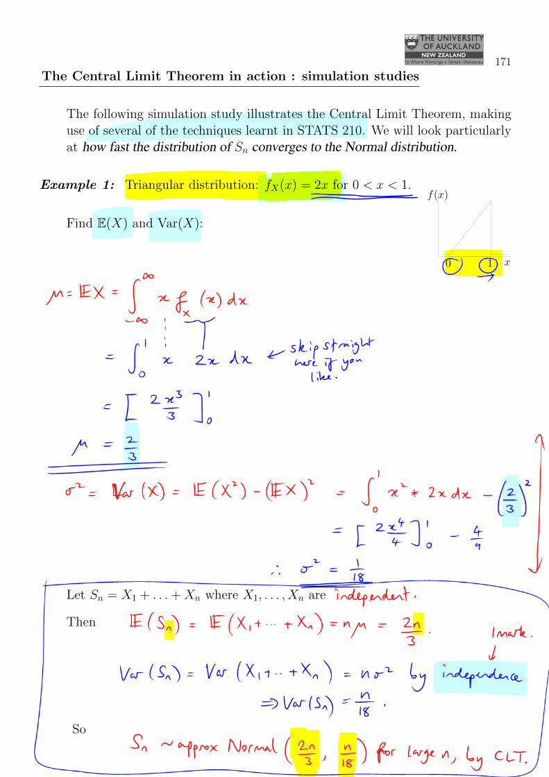
Example 1: Triangular distribution: fX(x) = 2x for 0 < x < 1.

x

f(x)

0 1

Find E(X) and Var(X):

µ = E(X) =

∫ 1

0

xfX(x) dx

=

∫ 1

0

2x2 dx

=

[2x3

3

]1

0

=2

3.

σ2 = Var(X) = E(X2)− {E(X)}2

=

∫ 1

0

x2fX(x) dx−(

2

3

)2

=

∫ 1

0

2x3 dx− 4

9

=

[2x4

4

]1

0

− 4

9

=1

18.

Let Sn = X1 + . . .+Xn where X1, . . . , Xn are independent.

ThenE(Sn) = E(X1 + . . .+Xn) = nµ =

2n

3

Var(Sn) = Var(X1 + . . .+Xn) = nσ2 by independence

⇒ Var(Sn) =n

18.

So Sn ∼ approx Normal(

2n3 ,

n18

)for large n, by the Central Limit

Theorem.

172

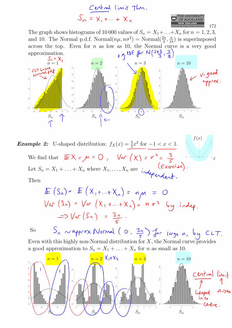
The graph shows histograms of 10 000 values of Sn = X1+. . .+Xn for n = 1, 2, 3,and 10. The Normal p.d.f. Normal(nµ, nσ2) = Normal(2n

3 ,n18) is superimposed

across the top. Even for n as low as 10, the Normal curve is a very goodapproximation.

0.0 0.2 0.4 0.6 0.8 1.0 1.2

0.0

0.5

1.0

1.5

2.0

n = 1

Sn

0.0 0.5 1.0 1.5 2.0

0.0

0.2

0.4

0.6

0.8

1.0

1.2

n = 2

Sn

0.5 1.0 1.5 2.0 2.5 3.0

0.0

0.2

0.4

0.6

0.8

1.0

n = 3

Sn

4 5 6 7 8 9

0.0

0.1

0.2

0.3

0.4

0.5

n = 10

Sn

Example 2: U-shaped distribution: fX(x) = 32x

2 for −1 < x < 1.

-1 10 x

f(x)

We find that E(X) = µ = 0, Var(X) = σ2 = 35. (Exercise)

Let Sn = X1 + . . .+Xn where X1, . . . , Xn are independent.

Then

E(Sn) = E(X1 + . . .+Xn) = nµ = 0

Var(Sn) = Var(X1 + . . .+Xn) = nσ2 by independence

⇒ Var(Sn) =3n

5.

So Sn ∼ approx Normal(0, 3n

5

)for large n, by the CLT.

Even with this highly non-Normal distribution for X, the Normal curve providesa good approximation to Sn = X1 + . . .+Xn for n as small as 10.

-1.0 -0.5 0.0 0.5 1.0

0.0

0.2

0.4

0.6

0.8

1.0

1.2

1.4

n = 1

Sn

-2 -1 0 1 2

0.0

0.2

0.4

0.6

n = 2

Sn

-3 -2 -1 0 1 2 3

0.0

0.1

0.2

0.3

0.4

n = 3

Sn

-5 0 5

0.0

0.05

0.10

0.15

n = 10

Sn

173

Normal approximation to the Binomial distribution, using the CLT

Let Y ∼ Binomial(n, p).

We can think of Y as the sum of n Bernoulli random variables:

Y = X1+X2+. . .+Xn, whereXi =

{1 if trial i is a “success” (prob = p),0 otherwise (prob = 1− p)

So Y = X1 + . . . + Xn and each Xi has µ = E(Xi) = p, σ2 = Var(Xi) =p(1− p).

Thus by the CLT,

Y = X1 +X2 + . . .+Xn → Normal(nµ, nσ2)

= Normal(np, np(1− p)

).

Thus,

Bin(n, p)→ Normal(

np︸︷︷︸mean of Bin(n,p)

, np(1− p)︸ ︷︷ ︸var of Bin(n,p)

)as n→∞ with p fixed.

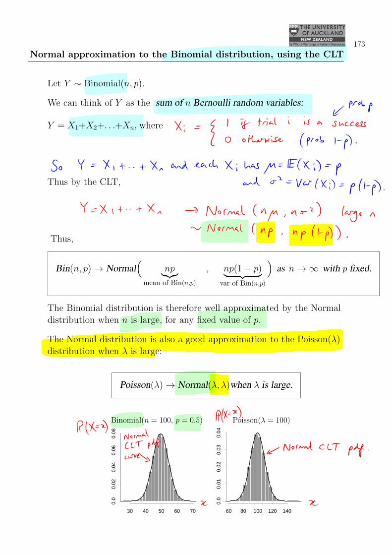
The Binomial distribution is therefore well approximated by the Normaldistribution when n is large, for any fixed value of p.

The Normal distribution is also a good approximation to the Poisson(λ)distribution when λ is large:

Poisson(λ)→ Normal(λ, λ)when λ is large.

30 40 50 60 70

0.0

0.02

0.04

0.06

0.08

60 80 100 120 140

0.0

0.01

0.02

0.03

0.04

Binomial(n = 100, p = 0.5) Poisson(λ = 100)

Why the Piece of Cake Theorem? . . .

• The Central Limit Theorem makes whole realms of statistics into a pieceof cake.

• After seeing a theorem this good, you deserve a piece of cake!

5.3 Confidence intervals

Example: Remember the margin of error for an opinion poll?

An opinion pollster wishes to estimate the level of support for Labour in anupcoming election. She interviews n people about their voting preferences. Letp be the true, unknown level of support for the Labour party in New Zealand.Let X be the number of of the n people interviewed by the opinion pollster whoplan to vote Labour. Then X ∼ Binomial(n, p).

At the end of Chapter 2, we said that the maximum likelihood estimator for pis

p̂ =X

n.

In a large sample (large n), we now know that

X ∼ approx Normal(np, npq) where q = 1− p.

So

p̂ =X

n∼ approx Normal

(p,

pq

n

)(linear transformation of Normal r.v.)

Sop̂− p√

pqn

∼ approx Normal(0, 1).

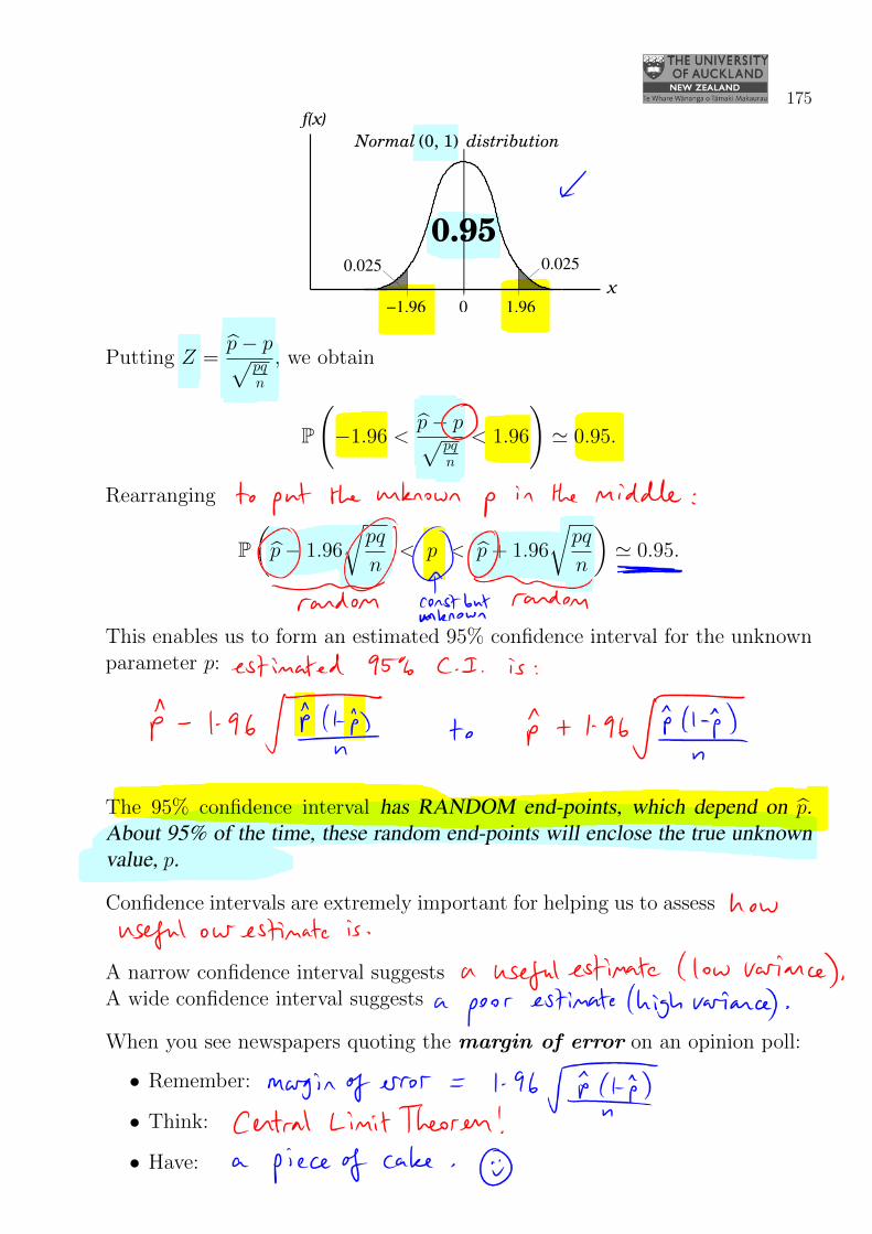
Now if Z ∼ Normal(0, 1), we find (using a computer) that the 95% centralprobability region of Z is from −1.96 to +1.96:

P(−1.96 < Z < 1.96) = 0.95.

Check in R: pnorm(1.96, mean=0, sd=1) - pnorm(-1.96, mean=0, sd=1)

175

Normal (0, 1) distribution

f(x)

0

x

0.0250.025

−1.96 1.96

0.95

Putting Z =p̂− p√

pqn

, we obtain

P

(−1.96 <

p̂− p√pqn

< 1.96

)' 0.95.

Rearranging to put the unknown p in the middle:

P(p̂− 1.96

√pq

n< p < p̂+ 1.96

√pq

n

)' 0.95.

This enables us to form an estimated 95% confidence interval for the unknownparameter p: estimated 95% confidence interval is

p̂− 1.96

√p̂(1− p̂)

nto p̂+ 1.96

√p̂(1− p̂)

n.

The 95% confidence interval has RANDOM end-points, which depend on p̂.About 95% of the time, these random end-points will enclose the true unknownvalue, p.

Confidence intervals are extremely important for helping us to assess how use-ful our estimate is.

A narrow confidence interval suggests a useful estimate (low variance);A wide confidence interval suggests a poor estimate (high variance).

When you see newspapers quoting the margin of error on an opinion poll:

• Remember: margin of error = 1.96√

p̂(1−p̂)n ;

• Think: Central Limit Theorem!

• Have: a piece of cake.

176

Confidence intervals for the Poisson λ parameter

We saw in section 3.6 that if X1, . . . , Xn are independent, identically distributedwith Xi ∼ Poisson(λ), then the maximum likelihood estimator of λ is

λ̂ = X =1

n

n∑

i=1

Xi.

Now E(Xi) = µ = λ, and Var(Xi) = σ2 = λ, for i = 1, . . . , n.

Thus, when n is large,

λ̂ = X ∼ approx Normal(µ,σ2

n)

by the Central Limit Theorem. In other words,

λ̂ ∼ approx Normal

(λ,

λ

n

)as n→∞.

We use the same transformation as before to find approximate 95% confidenceintervals for λ as n grows large:

Let Z =λ̂− λ√

λn

. We have Z ∼ approxNormal(0, 1) for large n.

Thus:

P

−1.96 <

λ̂− λ√λn

< 1.96

' 0.95.

Rearranging to put the unknown λ in the middle:

P

(λ̂− 1.96

√λ

n< λ < λ̂+ 1.96

√λ

n

)' 0.95.

So our estimated 95% confidence interval for the unknown parameter λ is:

λ̂− 1.96

√λ̂

nto λ̂+ 1.96

√λ̂

n.

177

Why is this so good?

It’s clear that it’s important to measure precision, or reliability, of an estimate,otherwise the estimate is almost worthless. However, we have already seenvarious measures of precision: variance, standard error, coefficient of variation,and now confidence intervals. Why do we need so many?

• The true variance of an estimator, e.g. Var(λ̂), is the most convenient quantityto work with mathematically. However, it is on a non-intuitive scale (squareddeviation from the mean), and it usually depends upon the unknown parameter,e.g. λ.

• The standard error is se(λ̂) =

√V̂ar

(λ̂)

. It is an estimate of the square

root of the true variance, Var(λ̂). Because of the square root, the standard erroris a direct measure of deviation from the mean, rather than squared deviationfrom the mean. This means it is measured in more intuitive units. However, itis still unclear how we should comprehend the information that the standarderror gives us.

• The beauty of the Central Limit Theorem is that it gives us an incredibly easyway of understanding what the standard error is telling us, using Normal-based asymptotic confidence intervals as computed in the previous twoexamples.

Although it is beyond the scope of this course to see why, the Central LimitTheorem guarantees that almost any maximum likelihood estimator will beNormally distributed as long as the sample size n is large enough, subject onlyto fairly mild conditions.

Thus, if we can find an estimate of the variance, e.g. V̂ar(λ̂), wecan immediately convert it to an estimated 95% confidence intervalusing the Normal formulation:

λ̂− 1.96

√V̂ar

(λ̂)

to λ̂+ 1.96

√V̂ar

(λ̂),

or equivalently,λ̂− 1.96 se(λ̂) to λ̂+ 1.96 se(λ̂) .

The confidence interval has an easily-understood interpretation: on 95% ofoccasions we conduct a random experiment and build a confidenceinterval, the interval will contain the true parameter.

So the Central Limit Theorem has given us an incredibly simple and power-ful way of converting from a hard-to-understand measure of precision, se(λ̂),to a measure that is easily understood and relevant to the problem at hand.Brilliant!