Chapter 5 Symmetries and Conservation Lawssaeta/courses/p111/uploads/Y2011/HSChapter5.pdfChapter 5 Symmetries and Conservation Laws At a very fundamental level, physics is about identifying

Chapter 5

Symmetries and ConservationLaws

At a very fundamental level, physics is about identifying patterns of order in Na-ture. The inception of the field starts arguably with Tycho Brahe (1546-1601)— the first modern experimental physicist — and Johannes Kepler (1571-1630)— the first modern theoretical physicist. In the 16th century, Brahe collectedlarge amounts of astrophysical data about the location of planets and stars withgroundbreaking accuracy — using an impressive telescope set up in a castle. Keplerpondered for years over Brahe’s long tables of numbers until he could finally iden-tify a pattern underlying planetary dynamics: this was summarized in the threelaws of Kepler. Later on, Isaac Newton (1643-1727) referred to these achieve-ments through his famous quote: “If I have seen further it is only by standing onthe shoulders of giants”.

Since then, physics has always been about identifying patterns in numbers,in measurements. And a pattern is simply an indication of a repeating rule, aconstant attribute in complexity, an underlying symmetry. In 1918, Emmy Noether(1882–1935) published a seminal work that clarified the deep relations betweensymmetries and conserved quantities in Nature. In a sense, this work organizesphysics in a clear diagram and gives one a bird’s eye view of the myriad of branchesof the field. Noether’s theorem, as it is called, can change the way one thinks aboutphysics in general. It is profound yet simple.

While one can study Noether’s theorem in the Newtonian formulation of me-chanics through cumbersome methods, the subject is an excellent demonstration ofthe power of the new formalism we developed, Lagrangian mechanics. In this sec-tion, we use the variational principle to develop a statement of Noether’s theorem.We then prove it and demonstrate its importance through examples.

189

190 CHAPTER 5. SYMMETRIES AND CONSERVATION LAWS

Figure 5.1: Two particles on a rail.

EXAMPLE 5-1: A simple example

Let us start with a simple mechanics problem from an example we saw inSection 4.1. We have two particles, with masses m

1

and m2

, confined to movingalong a horizontal frictionless rail as depicted in Figure 5. The action for thesystem is

S =Z

dt

✓12m

1

q2

1

+12m

2

q2

2

� V (q1

� q2

)◆

(5.1)

where we are considering some interaction between the particles described by apotential V (q

1

� q2

) that depends only on the distance between the particles.Let us consider a simple transformation of the coordinates given by

q01

= q1

+ C , q02

= q2

+ C (5.2)

where C is some arbitrary constant. We then have

q01

= q1

, q02

= q2

. (5.3)

Hence, the kinetic terms in the action are unchanged under this transformation.Furthermore, we also have

q01

� q02

= q1

� q2

(5.4)

5.1. INFINITESIMAL TRANSFORMATIONS 191

implying that the potential term is also unchanged. The action then preserves itsoverall structural form under the transformation

S !Z

dt

✓12m

1

q02

1

+12m

2

q02

2

� V (q01

� q02

)◆

. (5.5)

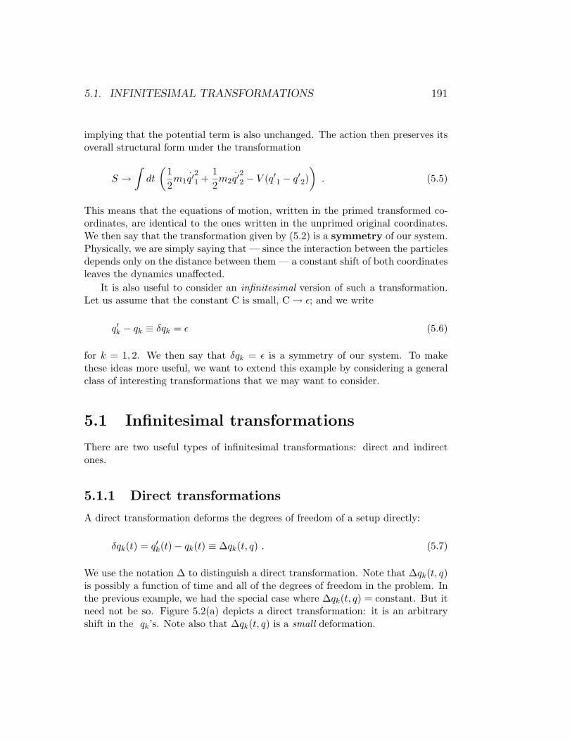
This means that the equations of motion, written in the primed transformed co-ordinates, are identical to the ones written in the unprimed original coordinates.We then say that the transformation given by (5.2) is a symmetry of our system.Physically, we are simply saying that — since the interaction between the particlesdepends only on the distance between them — a constant shift of both coordinatesleaves the dynamics una↵ected.

It is also useful to consider an infinitesimal version of such a transformation.Let us assume that the constant C is small, C! ✏; and we write

q0k � qk ⌘ �qk = ✏ (5.6)

for k = 1, 2. We then say that �qk = ✏ is a symmetry of our system. To makethese ideas more useful, we want to extend this example by considering a generalclass of interesting transformations that we may want to consider.

5.1 Infinitesimal transformations

There are two useful types of infinitesimal transformations: direct and indirectones.

5.1.1 Direct transformations

A direct transformation deforms the degrees of freedom of a setup directly:

�qk(t) = q0k(t)� qk(t) ⌘ �qk(t, q) . (5.7)

We use the notation � to distinguish a direct transformation. Note that �qk(t, q)is possibly a function of time and all of the degrees of freedom in the problem. Inthe previous example, we had the special case where �qk(t, q) = constant. But itneed not be so. Figure 5.2(a) depicts a direct transformation: it is an arbitraryshift in the qk’s. Note also that �qk(t, q) is a small deformation.


Figure 5.2: The two types of transformations considered: direct on the left,indirect on the right.

5.1.2 Indirect transformations

In contrast, an indirect transformation a↵ects the degrees of freedom indirectly —through the transformation of the time coordinate:

�t(t, q) ⌘ t0 � t . (5.8)

Note again that the shift in time can depend on time and the degrees of freedom aswell! It is again assumed to be small. This is however not the end of the story sincethe degrees of freedom depend on time and will get a↵ected as well — indirectly

qk(t) = qk(t0 � �t) ' qk(t0)� dqk

dt0�t ' qk(t0)� qk�t (5.9)

where we have used a Taylor expansion in �t to linear order since �t is small. Wealso have used dqk/dt0 = dqk/dt since this term already multiplies a power of �t:to linear order in �t, �t dqk/dt0 = �t dqk/dt ⌘ �t qk. We then see that shifting timeresults in a shift in the degrees of freedom

�qk = qk(t0)� qk(t) = q �t(t, q) . (5.10)

Figure 5.2(b) shows how you can think of this e↵ect graphically.

5.1. INFINITESIMAL TRANSFORMATIONS 193

5.1.3 Combined transformations

In general, we want to consider a transformation that may include both direct andindirect pieces. We would write

�qk = q0k(t0)� qk(t) = q0k(t

0) + [�qk(t0) + qk(t0)]� qk(t)= [q0k(t

0)� qk(t0)] + [qk(t0)� qk(t)] = �qk(t0, q) + q �t(t, q)= �qk(t, q) + q �t(t, q) . (5.11)

where in the last line we have equated t and t0 since the first term is already linearin the small parameters. To specify a particular transformation, we would thenneed to provide a set of functions

�t(t, q) and �qk(t, q) . (5.12)

Equation (5.11) then determines �qk(t, q). For N degrees of freedom, that’s N +1functions of time and the qk’s. Let us look at a few examples.

EXAMPLE 5-2: Translations

Consider a single particle in three dimensions, described by the three Cartesiancoordinates x1 = x, x2 = y, and x3 = z. We also have the time coordinate x0 = c t.An infinitesimal spatial translation can be realized by

�xi(t, x) = ✏i , �t(t, x) = 0) �xi(t, x) = ✏i (5.13)

where i = 1, 2, 3, and the ✏i’s are three small constants. A translation in space isthen defined by

{�t(t, x) = 0, �xi(t, x) = ✏i} (5.14)

A translation in time on the other hand would be given by

�xi(t, x) = 0 , �t(t, x) = ") �xi(t, x) = �xi" (5.15)

for constant ". Notice that we require that the total shifts in the xi’s — the�xi(t, x)’s — vanish. This then generates direct shifts, the �xi’s, to compensatefor the indirect e↵ect on the spatial coordinates from the shifting of the time. Atranslation in time is then defined by

{�t(t, x) = ✏, �xi(t, x) = 0} (5.16)


EXAMPLE 5-3: Rotations

To describe rotations, let us consider a particle in two dimensions for simplicity.We use the coordinates x1 = x and x2 = y. We start by specifying

�t(t, x) = 0) �xi(t, x) = �xi(t, x) . (5.17)

Next, we look at an arbitrary rotation angle ✓ using (2.21)✓x1

0

x2

0

◆=✓

cos ✓ sin ✓� sin ✓ cos ✓

◆✓x1

x2

◆. (5.18)

We however need to focus on an infinitesimal version of this transformation: i.e.we need to consider small angle ✓. Using cos ✓ ⇠ 1 and sin ✓ ⇠ ✓ to second orderin ✓, we then write✓

x1

0

x2

0

◆=✓

1 ✓�✓ 1

◆✓x1

x2

◆. (5.19)

This gives

�x1(t, x) = x1

0(t)� x1(t) = ✓ x2(t) = �x1(t, x)

�x2(t, x) = x2

0(t)� x2(t) = �✓ x1(t) = �x2(t, x) . (5.20)

We see we have a more non-trivial transformation. Rotations can then be definedthrough

{�t(t, x) = 0, �xi(t, x) = ✓ "ijxj(t)} (5.21)

where j is summed over 1 and 2. We have also introduced a useful shorthand: "ij .It is called the totally antisymmetric matrix in two dimensions and defined as:

"11 = "22 = 0 , "12 = �"21 = 1 . (5.22)

It allows us to write the transformation in a more compact notation.

EXAMPLE 5-4: Lorentz transformationsTo find the infinitesimal form of Lorentz transformations, we can start with thegeneral transformation equations (2.15) and take � small. We need to be carefulhowever to keep the leading order terms in � in all expansions. Given our previousexample, it is easier to map the problem onto a rotation with hyperbolic trigfunctions using (2.27). For simplicity, let us consider a particle in one dimension,

5.2. SYMMETRY 195

with two relevant coordinates x0 = c t and x1. Looking back at (2.27), we takethe rapidity ⇠ to be small and use cosh ⇠ ⇠ 1 and sinh ⇠ ⇠ ⇠ to linear order in ⇠.Along the same steps of the previous example, we quickly get

�x0(t, x) = ⇠ x1 , �x1(t, x) = ⇠ x0 . (5.23)

Using equation (5.11), we then have

�x1(t, x) = �x1(t, x)� x1�t(t, x) = ⇠ c t� ⇠

cx1x1 . (5.24)

Note that we have

sinh ⇠ = �� ) sinh ⇠ ⇠ ⇠ ⇠ � . (5.25)

Lorentz transformations can then be written through

{�x0(t, x) = � x1 , �x1(t, x) = � x0 , �x2(t, x) = �x3(t, x) = 0} (5.26)

where we added the transverse directions to the game as well.

5.2 Symmetry

At the beginning of this section, we defined symmetry as a transformation thatleaves the action unchanged in form. In that particular example of two interactingparticles on a wire, it was simple to see that the transformation was indeed asymmetry. Now that we have a general class of transformations, we want to finda general condition that can be used to test whether a particular transformation,possibly a complicated one, is a symmetry or not. We then need to look at howthe action changes under a general transformation; for a symmetry, this changeshould vanish. We start with the usual form for the action

S =Z

dt L(q, q, t) . (5.27)

And we apply a general transformation given by �qk(t, q) and �t(t, q). We thenhave

�S =Z�(dt) L +

Zdt �(L) , (5.28)

where we used the Leibniz rule of derivation since � is an infinitesimal change. Thefirst term is the change in the measure of the integrand

�(dt) = dt�(dt)dt

= dtd

dt(�t) . (5.29)


In the last bit, we have exchanged the order of derivations since derivations com-mute. The second term has two pieces

�(L) = �(L) + �tdL

dt. (5.30)

The first piece is the change in L resulting from its dependence on the qk’s andqk’s. Hence, we labeled it as a direct change with a �. The second piece is thechange in L to linear order in �t due to the change in t. This comes from changesin the qk’s on which L depends, as well as changes in t directly since t can makean explicit appearance in L. This is an identical situation to the linear expansionencountered for qk in (5.11): there’s a piece from direct changes in the degrees offreedom, plus a piece from the transformation of time. We can further write

�(L) =@L

@qk�qk +

@L

@qk�(qk) =

@L

@qk�qk +

@L

@qk

d

dt(�qk) . (5.31)

Note that in the last term, we exchanged the orders of derivations, � and d/dt:derivations are commutative. We can now put everything together and write

�S =Z

dt

✓@L

@qk�qk +

@L

@qk

d

dt(�qk) + �t

dL

dt+ L

d

dt(�t)

◆=

Zdt

✓@L

@qk�qk +

@L

@qk

d

dt(�qk) +

d

dt(L �t)

◆. (5.32)

Given L, �t(t, q), and �qk(t, q), we can substitute these in (5.32) and check whetherthe expression vanishes. If it does vanish, we conclude that the given transforma-tion {�t(t, q),�qk(t, q)} is a symmetry of our system. This shall be our notion ofsymmetry. A bit later, we will revisit this statement and generalize it further. Fornow, this is enough to move onto the heart of the topic, Noether’s theorem.

5.2.1 Noether’s theorem

The theorem

We start by simply stating the theorem:For every symmetry {�t(t, q),�qk(t, q}, there exists a quantity that is conserved

under time evolution.A symmetry implies a conservation law. This is important for two reasons.

(1) First, a conservation law identifies a rule in the laws of Physics. Virtuallyeverything we have a name for physics — mass, momentum, energy, charge, etc..— is tied by definition to a conservation law. Noether’s theorem then states thatfundamental physics is founded on the principle of identifying the symmetries of

5.2. SYMMETRY 197

Nature. If one wants to know all the laws of physics, one needs to ask: what are allthe symmetries in Nature. From there, you find conservation laws and associatedinteresting conserved quantities. You then can study how these conservation lawscan be violated. This leads you to equations that you can use to predict the futurewith. It’s all about symmetries. (2) Second, conservation laws have the form

d

dt(Something) = 0) Something = Constant . (5.33)

The ‘Something’ is typically a function of the degrees of freedom and the firstderivatives of the degrees of freedom. The conservation statement then inherentlyleads to first order di↵erential equations. First order di↵erential equations aremuch nicer than second or higher order ones. Thus, technically, finding the sym-metries and corresponding conservation laws in a problem helps a great deal insolving and understanding the physical system.

The easiest way to understand Noether’s theorem is to prove it, which is asurprisingly simple exercise.

Proof of Noether’s theorem

The premise of the theorem is that we have a given symmetry {�t(t, q),�qk(t, q}.This then implies, using (5.32), that we have

�S = 0 =Z

dt

✓@L

@qk�qk +

@L

@qk

d

dt(�qk) +

d

dt(L �t)

◆. (5.34)

Note that we know that this equation is satisfied for any set of curves qk(t) byvirtue of {�t(t, q),�qk(t, q} constituting a symmetry. And now comes the crucialstep: what if the qk(t)’s satisfied the equations of motion

d

dt

✓@L

@qk

◆=@L

@qk. (5.35)

Of all possible curves qk(t), we pick the ones that satisfy the equations of motion.Given this additional statement, we can rearrange the terms in �S such that

0 =Z

dtd

dt

✓@L

@qk�qk + L �t

◆. (5.36)

Since the integration interval is arbitrary, we then conclude that

d

dt(Q) = 0 (5.37)


with

Q ⌘ @L

@qk�qk + L �t ; (5.38)

We have a conserved quantity. Q is called the Noether charge. Note a fewimportant points:

• We used the equations of motion to prove the conservation law. However,we did not use the equations of motion to conclude that a particular trans-formation is a symmetry. The symmetry exists at the level of the action forany qk(t). The conservation law exists for physical trajectories that satisfythe equations of motion.

• The proof identifies explicitly the conserved quantity through (5.38). Know-ing L, �t(t, q), and �qk(t, q), this equation tells us immediately the conservedquantity associated with the given symmetry.

This proof also highlights a route to generalize the original definition of sym-metry. All that was needed was to have

�S =Z

dtd

dt(K) (5.39)

where K is some function that you would find out by using (5.32). If K turns outto be a constant, we would get �S = 0 and we are back to the situation at hand.However, if K is non-trivial, we would get

�S =Z

dtd

dt(K) =

Zdt

d

dt

✓@L

@qk�qk + L �t

◆. (5.40)

This now means thatd

dt(Q�K) = 0 (5.41)

and hence the conserved quantity is Q � K instead of Q. Since the interestingconceptual content of a symmetry is its associated conservation law, we want toturn the problem on its back: we want to define a symmetry through a conservationstatement. So, here’s a revised more general statement

{�t(t, q),�qk(t, q} is a symmetry if �S =Z

dtdK

dtfor some K . (5.42)

Noether’s theorem then states that for every such symmetry, there is a conservedquantity given by Q�K.

To summarize, here’s then the general prescription:

5.2. SYMMETRY 199

1. Given a Lagrangian L and a candidate symmetry {�t(t, q),�qk(t, q}, use (5.32)to find �S. If �S =

Rdt dK/dt for some K you are to determine, {�t(t, q),�qk(t, q}

is indeed a symmetry.

2. If {�t(t, q),�qk(t, q} was found to be a symmetry with some K, we can findan associated conserved quantity Q�K, with Q given by (5.38).

Let us look at a few examples.

EXAMPLE 5-5: Space translations and momentum

We start with the spatial translation transformation from our previous exam-ple (5.13)

�xi(t, x) = ✏i , �t(t, x) = 0) �xi(t, x) = ✏i . (5.43)

We next need a Lagrangian to test this transformation against. Consider first

L =12mxixi . (5.44)

We substitute (5.43) and (5.44) into (5.32) and easily find

�S = 0) K = Constant. (5.45)

Hence, we have a symmetry at hand. To find the associated conserved charge, weuse (5.38) and find

Qi = mxi✏i No sum on i. (5.46)

We then have three charges for the three possible directions for translation. Anoverall additive or multiplicative constant is arbitrary since it does not a↵ect thestatement of conservation Qi = 0. Writing the conserved quantities as P i instead,we state

P i = mxi (5.47)

i.e. momentum is the Noether charge associate with the symmetry of spatialtranslational invariance. If we have a physical system set up on a table and wenotice that we can move the table by any amount in any of the three spatialdirections without a↵ecting the dynamics of the system, we can conclude thatthere is a quantity — called momentum by definition — that remains constant intime.


We can then try to find the conditions under which this symmetry, and henceconservation law, is violated. For example, we could consider a setup which resultsin adding a familiar potential term to the Lagrangian

L =12mxixi � 1

2k xixi . (5.48)

Using (5.32), we now get

�S =Z

dt��k xi✏i

� 6= Z d

dt(K) . (5.49)

Hence, momentum is not conserved and we would write

P i 6= 0) P i ⌘ F i (5.50)

thus introducing the concept of ‘force’. You now see that the second law of Newtonis nothing but a reflection of the existence or non-existence of a certain symmetryin Nature.

Newton’s third law is also related to this idea: action-reaction pairs canceleach other so that the total force on an isolated system is zero and hence the totalmomentum is conserved. To see this, look back at the two particle system on arail described by the Lagrangian (4.69). Using once again (5.32), we get

�S = 0) P i = m1

q1

+ m2

q2

; (5.51)

Thus, total momentum is our Noether charge and it is conserved. The forceson each particle are �@V/@q

1

and �@V/@q2

, which are equal in magnitude butopposite in sign since we have V (q

1

� q2

) — note the relative minus sign betweenq1

and q2

@V (q1

� q2

)@q

1

= �@V (q1

� q2

)@q

2

. (5.52)

These two forces form the action-reaction pair. The cancelation of forces arisesbecause of the dependence of the potential and force on the distance q

1

�q2

betweenthe particles — which is what makes the problem translationally invariant as well.We now see that the third law is intimately tied to the statement of translationsymmetry.

EXAMPLE 5-6: Time translation and energy

5.2. SYMMETRY 201

Next, let us consider time translational invariance. Due to its particular useful-ness, we want to treat this example with greater generality. We focus on a systemwith an arbitrary number of degrees of freedom labeled by qk’s with a generalLagrangian L(q, q, t). We propose the transformation

�t = ✏ , �qk = 0 . (5.53)

Hence, the degrees of freedom are left unchanged, but the time is shifted by aconstant ✏. This means that we need a direct shift

�qk = 0 = �qk + qk�t = �qk + ✏ qk ) �qk = �✏ qk (5.54)

to compensate for the indirect change in qk induced by the shift in time. We thenuse (5.32) to find the condition for time translational symmetry

�S =Z

dt

✓�✏qk

@L

@qk� ✏qk

@L

@qk+ ✏

dL

dt

◆. (5.55)

But we also know

dL

dt=@L

@t+@L

@qkqk +

@L

@qkqk . (5.56)

We then get

�S =Z

dt@L

@t. (5.57)

In general, since L depends on the qk’s as well, we need to consider the morerestrictive condition for symmetry �S = 0, i.e. we have K = constant. Thisimplies that we have time translational symmetry if

@L

@t= 0 (5.58)

i.e. if the Lagrangian does not depend on time explicitly. If this is the case, wethen have a conserved quantity given by (5.38)

Q = �✏ qk@L

@qk+ ✏L . (5.59)

Dropping an overall constant term �✏ and rearranging, we write

Q! H = qk@L

@qk� L . (5.60)


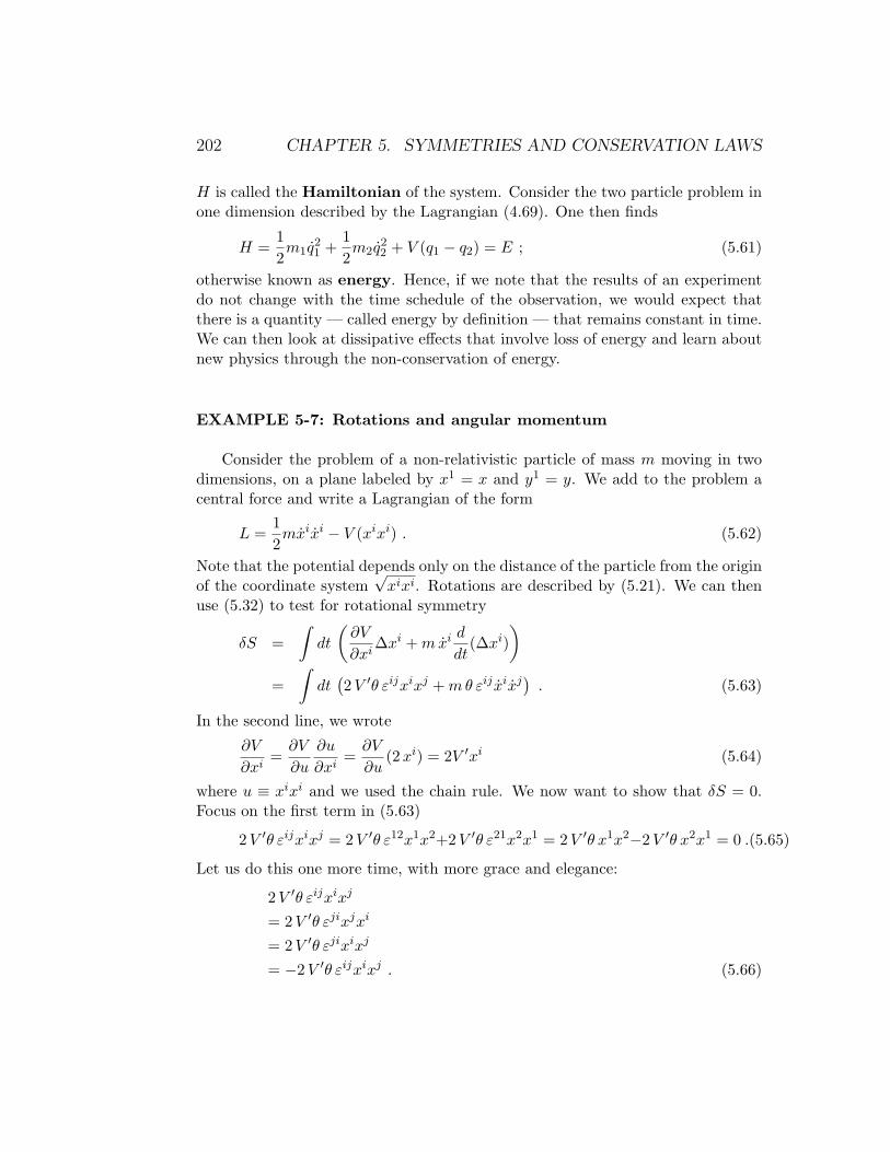
H is called the Hamiltonian of the system. Consider the two particle problem inone dimension described by the Lagrangian (4.69). One then finds

H =12m

1

q2

1

+12m

2

q2

2

+ V (q1

� q2

) = E ; (5.61)

otherwise known as energy. Hence, if we note that the results of an experimentdo not change with the time schedule of the observation, we would expect thatthere is a quantity — called energy by definition — that remains constant in time.We can then look at dissipative e↵ects that involve loss of energy and learn aboutnew physics through the non-conservation of energy.

EXAMPLE 5-7: Rotations and angular momentum

Consider the problem of a non-relativistic particle of mass m moving in twodimensions, on a plane labeled by x1 = x and y1 = y. We add to the problem acentral force and write a Lagrangian of the form

L =12mxixi � V (xixi) . (5.62)

Note that the potential depends only on the distance of the particle from the originof the coordinate system

pxixi. Rotations are described by (5.21). We can then

use (5.32) to test for rotational symmetry

�S =Z

dt

✓@V

@xi�xi + m xi d

dt(�xi)

◆=

Zdt�2 V 0✓ "ijxixj + m ✓ "ij xixj

�. (5.63)

In the second line, we wrote@V

@xi=@V

@u

@u

@xi=@V

@u(2 xi) = 2V 0xi (5.64)

where u ⌘ xixi and we used the chain rule. We now want to show that �S = 0.Focus on the first term in (5.63)

2 V 0✓ "ijxixj = 2V 0✓ "12x1x2+2V 0✓ "21x2x1 = 2V 0✓ x1x2�2 V 0✓ x2x1 = 0 .(5.65)

Let us do this one more time, with more grace and elegance:

2 V 0✓ "ijxixj

= 2V 0✓ "jixjxi

= 2V 0✓ "jixixj

= �2 V 0✓ "ijxixj . (5.66)

5.2. SYMMETRY 203

In the second line, we just relabeled the indices i ! j and j ! i: since they aresummed indices, it does not matter what they are called. In the third line, we usethe fact that multiplication is commutative xjxi = xixj . Finally, in the third line,we used the property "ij = �"ji from (5.22). Hence, we have shown

2 V 0✓ "ijxixj = �2 V 0✓ "ijxixj ) 2 V 0✓ "ijxixj = 0 . (5.67)

The key idea is that "ij is antisymmetric in its indices while xixj is symmetricunder the same indices. The sum of their product then cancels. The same is truefor the second term in (5.63)

m ✓ "ij xixj = �m ✓ "ij xixj ) m ✓ "ij xixj = 0 . (5.68)

We will use this trick occasionally later on in other contexts. We thus have shownthat our system is rotational symmetric

�S = 0) K = Constant . (5.69)

We can then determine the conserved quantity using (5.38)

Q =@L

@xi�xi = m xi✓ "ijxj . (5.70)

Dropping a constant term ✓, we write

l = m "ij xixj = m�x1x2 � x2x1

�= (~r⇥m ~v)z (5.71)

i.e. this is the z-component of the angular momentum of the particle; it pointsperpendicular to the plane of motion as expected. Rotational symmetry impliesconservation of angular momentum. Rotation about the z axis corresponds toangular momentum along the z axis.

EXAMPLE 5-8: Lorentz and Galilean BoostsHow about a Lorentz transformation? The Relativity postulate requires the Lorentztransformation as a symmetry of any physical system: it is not a question ofwhether it is a symmetry of a given system; it better be! We could then use (5.32),with Lorentz transformations, as a condition for sensible Lagrangians. Noether’stheorem can be used to construct theories consistent with the required symmetries.In general, an experiment would identify a set of symmetries in a newly discov-ered system. Then the theorist’s task is to build a Lagrangian that describes thesystem; and a good starting point would be to assure that the Lagrangian has allthe needed symmetries. You now see the power of Noether’s theorem: it allowsyou to mold equations and theories to your needs.


Coming back to Lorentz transformations, let us look at an explicit exampleand find the associated conserved charge. We would consider a relativistic system,say a free relativistic particle with action

S = �mc2

Zd⌧ = �mc2

Z r1� xixi

c2

. (5.72)

A particular Lorentz transformation is given by (5.26) which we can then substitutein (5.32) to show that we have a symmetry. However, this is an algebraicallycumbersome exercise that we would prefer to leave as a homework problem forthe reader. It is more instructive to simplify the problem further. Hence, weconsider instead the small speed limit, i.e. we consider a non-relativistic systemwith Galilean symmetry. We take a single free particle in one dimension withLagrangian

L =12mx2 . (5.73)

The expected symmetry is Galilean, given by (1.1) which we quote again for con-venience

x = x0 + V t0 , y = y0 , z = z0 , t = t0 . (5.74)

We can then write the infinitesimal version quickly

�t = �y = �z = 0 , �x = �V t

) �t = �y = �z = 0 and �x = �V t . (5.75)

Note that we want to think of this transformation near t ⇠ 0, the instant in timethe two origins coincide, to keep it as a small deformation for any V . Using (5.32),we then get

�S =Z

dt m V x . (5.76)

Before we panic from the fact that this did not vanish, let us remember that allthat is needed is �S =

Rdt dK/dt for some K. That is indeed the case

�S =Z

dtd

dt(m V x) . (5.77)

We then have

K = m V x + Constant . (5.78)

5.2. SYMMETRY 205

The system then has Galilean symmetry. We look at the associated Noether chargeusing (5.38)

Q =@L

@x�x = m xV t . (5.79)

But this is not the conserved charge: Q�K is the conserved quantity

Q�K = m xV t�m V x = Constant . (5.80)

Rewriting things, we have a simple first order di↵erential equation

x t� x = Constant . (5.81)

Integrating this gives the expected linear trajectory x(t) / t. Unlike momentum,energy, and angular momentum, this conserved quantity Q � K is not given itsown glorified name. Since Galilean (or the more general Lorentz) symmetry isexpected to be prevalent in all systems, this does not add any useful distinguishingphysics ingredient to a problem. Perhaps if we were to discover a fundamentalphenomenon that breaks Galilean/Lorentz symmetry, we could then revisit thisconserved quantity and study its non-conservation. For now, this conserved chargegets relegated to second rate status...

EXAMPLE 5-9: Sculpting Lagrangians from symmetry

Let us take the previous example one step further. What if we were to requirea symmetry and ask for all possible Lagrangians that fit the mold. To be morespecific, consider a one dimensional system with one degree of freedom, denoted asq(t). We want to ask: what are all possible theories that can describe this systemwith the following conditions: they are to be Galilean invariant and invariant undertime translations. The Galilean symmetry is obtained from (5.75) in the previousexample

�t = 0 and �x = �x = �V t . (5.82)

Substituting this into (5.32), we get

�S =Z

dt

✓�@L

@xV t� @L

@xV

◆=Z

dtd

dt(K) . (5.83)

The question is then to find the most general L that does the job for some K.This means we need

@L

@xt +

@L

@x/ d

dt(K)! d

dt

⇣ eK⌘ , (5.84)


where we absorbed the proportionality constant inside the yet to be determinedfunction eK. Note also that we are not allowed to use the equations of motion!Using the chain rule with eK(t, x, x, x, . . .), we can write

d

dt

⇣ eK⌘ =@ eK@t

+@ eK@x

x +@ eK@x

x + . . . (5.85)

Comparing this to (5.84), we see that we need eK(t, x) — a function of t and xonly — since we know L is a function of t, x, and x only; hence we have

@L

@xt +

@L

@x=@ eK@t

+@ eK@x

x . (5.86)

We want a general form for L, yet eK(t, x) is also arbitrary. Since the right-handside is linear in x, so must be the left hand side. This implies we need L to be aquadratic polynomial in x

L = f1

(t, x)x2 + f2

(t, x)x + f3

(t, x) (5.87)

with three unknown functions f1

(t, x), f2

(t, x), and f3

(t, x). Looking at the @L/@xterm, we can immediately see that we need f

1

(t, x) = C1

, a constant independentof x and t: otherwise we generate a term quadratic in x that does not exist on theright-hand side of (5.86). Our Lagrangian now looks like

L = C1

x2 + f2

(t, x)x + f3

(t, x) . (5.88)

But we forgot about the time translational symmetry. That, we know, requiresthat @L/@t = 0. We then should write instead

L = C1

x2 + f2

(x)x + f3

(x) . (5.89)

But the second term is irrelevant to the dynamics. This is because L will appearin the action integrated over time; and this second term can be integrated outZ

dt f2

(x)x =Z

dtd

dt(F

2

(x)) = F2

(x)|boundaries (5.90)

for some function F2

(x) =R x

d⇠ f2

(⇠). Hence the term does not depend on theshape of paths plugged into the action functional and cannot contribute to thestatement of extremization — otherwise known as the equation of motion. We arenow left with

L! C1

x2 + f3

(x) . (5.91)

5.2. SYMMETRY 207

The condition (5.86) on L now looks like

@f3

(x)@x

t + 2 C1

x =@ eK@t

+@ eK@x

x . (5.92)

Picking out the x dependences on either sides, this implies

2 C1

=@ eK@x

,@f

3

(x)@x

t =@ eK@t

. (5.93)

Since we know that

@2 eK@x@t

=@2 eK@t@x

, (5.94)

di↵erentiating the two equations in (5.93) leads to the condition

@2f3

(x)@x2

= 0) f3

(x) = C2

x + C3

(5.95)

for some constants C2

and C3

. The Lagrangian now looks like

L = C1

x2 + C2

x , (5.96)

where we set C3

= 0 since a constant shift of L does not a↵ect the equation ofmotion. We can now solve for eK as well if we wanted to using (5.93)

eK = 2C1

x +C

2

2t2 + Constant . (5.97)

Now, let us stare back at the important point, equation (5.96). We write theconstants C

1

and C2

as C1

= m/2 and C2

= �m g

L =12mx2 �m g x . (5.98)

With tears of joy in our eyes, we just showed that the most general Galilean andtime translation invariant mechanics problem in one dimension necessarily lookslike a particle in uniform gravity. We were able to derive the canonical kineticenergy term and gravitational potential from a symmetry requirement. This isjust a hint at the power of symmetries and conservation laws in physics. Indeed,all the known forces of Nature can be derived from first principles from symmetries!

EXAMPLE 5-10: Generalized momenta and cyclic coordinates


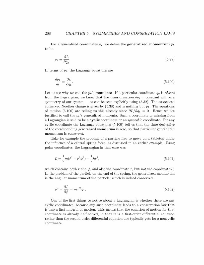
For a generalized coordinates qk, we define the generalized momentum pk

to be

pk ⌘ @L

@qk. (5.99)

In terms of pk, the Lagrange equations are

dpk

dt=@L

@qk. (5.100)

Let us see why we call the pk’s momenta. If a particular coordinate qk is absentfrom the Lagrangian, we know that the transformation �qk = constant will be asymmetry of our system — as can be seen explicitly using (5.32). The associatedconserved Noether charge is given by (5.38) and is nothing but pk. The equationsof motion (5.100) are telling us this already since @L/@qk = 0. Hence we arejustified to call the pk’s generalized momenta. Such a coordinate qk missing froma Lagrangian is said to be a cyclic coordinate or an ignorable coordinate. For anycyclic coordinate the Lagrange equations (5.100) tell us that the time derivativeof the corresponding generalized momentum is zero, so that particular generalizedmomentum is conserved.

Take for example the problem of a particle free to move on a tabletop underthe influence of a central spring force, as discussed in an earlier example. Usingpolar coordinates, the Lagrangian in that case was

L =12m(r2 + r2'2)� 1

2kr2, (5.101)

which contains both r and ', and also the coordinate r, but not the coordinate '.In the problem of the particle on the end of the spring, the generalized momentumis the angular momentum of the particle, which is indeed conserved

p' =@L

@'= m r2 ' . (5.102)

One of the first things to notice about a Lagrangian is whether there are anycyclic coordinates, because any such coordinate leads to a conservation law thatis also a first integral of motion. This means that the equation of motion for thatcoordinate is already half solved, in that it is a first-order di↵erential equationrather than the second-order di↵erential equation one typically gets for a noncycliccoordinate.

5.2. SYMMETRY 209

5.2.2 Some comments on symmetries

Let us step back for a moment and comment on several additional issues aboutsymmetries and conservation laws.

• If a system has N degrees of freedom, then the typical Lagrangian leads toN second order di↵erential equations (provided the Lagrangian depends onat most first derivatives of the variables). If we were lucky enough to solvethese equations, we would parameterize the solution with 2 N constantsrelated to the boundary conditions. If our system has M symmetries, itwould then have M conserved quantities. Each of the symmetries leadsto a first order di↵erential equation, and hence a total of M constants ofmotion. In total, the conservation equations will gives has 2M constantsto parameterize the solution with: M from the constants of motion, andanother M for integrating the first order equations. These 2M constantswould necessarily be related to the 2 N constants mentioned earlier. Whatif we have M = N? The system is then said to be integrable. This meansthat all one needs to do is to write the conservation equations and integratethem. We need not even stare at any second order di↵erential equations tofind the solution to the dynamics. In general, we will have M N . Andthe closer M is to N , the easier will be to understand the given physicalproblem. As soon as a good physicist sees a physics problem, he or shewould first count degrees of freedom; then he or she would instinctively lookfor the symmetries and associated conserved charges. This immediately laysout a strategy how to tackle the problem based on how much symmetriesone has versus the number of degrees of freedom.

• Noether’s theorem is based on infinitesimal transformations: symmetriesthat can be build up from small incremental steps of deformations. Thereare other symmetries in Nature that do not fit this prescription. For ex-ample, discrete symmetries are rather common. Reflection transformations,e.g. time reflection t! �t or discrete rotations of a lattice, can be very im-portant for understanding the physics of a problem. Noether’s theorem doesnot apply to these. However, such symmetries are also often associated withconserved quantities. Sometimes, these are called topological conservationlaws.

• Infinitesimal transformations can be catalogued rigorously in mathematics.A large and useful class of such transformations fall under the topic of Liegroups of Group theory. The Lie group catalogue (developed by Cartan) isexhaustive. Many if not all of the entries in the catalogue are indeed realizedin Nature in various physical systems. In addition to Lie groups, physicists


also flirt with other more exotic symmetries such as supersymmetry. Albeitmathematically very beautiful, unfortunately none of these will be of interestto us in mechanics.

5.3 Exercises and Problems

PROBLEM 5-1 :Consider a particle of mass m moving in two dimensions in the x � y plane,

constrained to a rail-track whose shape is describe by an arbitrary function y =f(x). There is NO GRAVITY acting on the particle.

(a) Write the Lagrangian in terms of the x degree of freedom only.(b) Consider some general transformation of the form

�x = g(x) , �t = 0 ; (5.103)

where g(x) is an arbitrary function of x. Assuming that this transformation is asymmetry of the system such that �S = 0, show that this implies the followingdi↵erential equation relating f(x) and g(x)

g0

g= � 1

2(1 + f 02)d

dx

⇣f 0

2

⌘; (5.104)

where prime stands for derivative with respect to x (not t).(c) Write a general expression for the associated conserved charge in terms of

f(x), g(x), and x.(d) We will now specify a certain g(x), and try to find the laws of physics

obeying the prescribed symmetry; i.e. for given g(x), we want to find the shapeof the rail-track f(x). Let

g(x) =g0px

; (5.105)

where g0

is a constant. Find the corresponding f(x) such that this g(x) yields asymmetry. Sketch the shape of the rail-track. (HINT: h(x) = f 02.)

PROBLEM 5-2 : One of the most important symmetries in Nature is thatof Scale Invariance. This symmetry is very common (e.g. arises whenever asubstance undergoes phase transition), fundamental (e.g. it is at the foundationof the concept of Renormalization Group for which a physics Nobel Prize wasawarded in 1982), and entertaining (as you will now see in this problem).

5.3. EXERCISES AND PROBLEMS 211

Consider the action

S =Z

dtp

hq2 (5.106)

of two degrees of freedom h(t) and q(t).(a) Show that the following transformation (known as a scale transformation

or dilatation)

�q = ↵q , �h = �2↵h , �t = ↵t (5.107)

is a symmetry of this system.(b) Find the resulting constant of motion.

PROBLEM 5-3 :A massive particle moves under the acceleration of gravity and without friction

on the surface of an inverted cone of revolution with half angle ↵.(a) Find the Lagrangian in polar coordinates.(b) Provide a complete analysis of the trajectory problem. Use Noether charges

when useful.


Documents

Chapter 5 Symmetries and Conservation Lawssaeta/courses/p111/uploads/Y2011/HSChapter5.pdfChapter 5 Symmetries and Conservation Laws At a very fundamental level, physics is about identifying