Chapter 5Chapter 5

Satellite orbitsSatellite orbits

Remote Sensing of Ocean ColorInstructor: Dr. Cheng-Chien Liu

Department of Earth Science

National Cheng-Kung University

Last updated: 7 April 2003

Source: http://www.ioccg.org/training/turkey/DrLynch_lectures2.pdf

5.1 Introduction5.1 Introduction

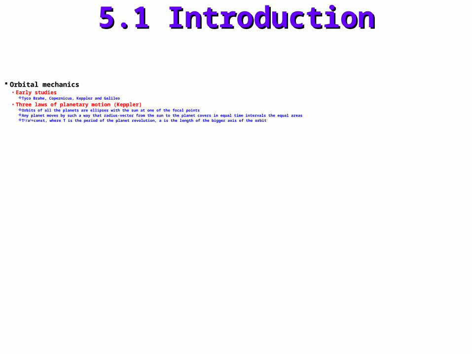
Orbital mechanicsOrbital mechanics• Early studies

Tyco Brahe, Copernicus, Keppler and Galileo

• Three laws of planetary motion (Keppler)Orbits of all the planets are ellipses with the sun at one of the focal pointsAny planet moves by such a way that radius-vector from the sun to the planet covers in equal time intervals the equal areasT2/a3=const, where T is the period of the planet revolution, a is the length of the bigger axis of the orbit

Fig 5.1.1Fig 5.1.1

Fig. 5.1.1 Historic satellite ocean color sensors Source: http://physics.nad.ru/Physics/English/mech.htm

5.1 Introduction (cont.)5.1 Introduction (cont.)

Orbital mechanics (cont.)Orbital mechanics (cont.)• The universal law of gravity (Newton 1666)

F = GmM/r2

Artificial earth orbiting satellite

• Sputnik (USSR 1957)

PerturbingPerturbing forces forces F = GmM/rF = GmM/r22 is not enough is not enough• Earth non-spherical shape• Ocean tides, atmospheric drag, Sun, …• Osculating orbit

5.1 Introduction (cont.)5.1 Introduction (cont.)

Orbit prediction modelOrbit prediction model• Why need?

Control and receiving dataGPS

• Ephemeris = fn(t)Help us to determine the orbit based on the goals of satellite mission

5.2 Terminology and coordinate 5.2 Terminology and coordinate systemssystems

Coordinate systemCoordinate system• Geodetic• Geocentric using this system

Origin: center of massAxis 1: ON (Origin to North Pole)Axis 2: OA (Aries)Axis 3: ON && OA

Aries: Aries is a point in space the direction of which is determined by the intersection of the equatorial plane of the Earth (ie the plane that contains the equator) and the orbital plane defined by the Earth’s annual motion around the Sun ( see Figure 1.1) such that a line from the Sun’s centre to the Earth along this direction points toward Aries at the time of the Vernal Equinox. This latter event occurs at a date near March 20 each year when the Sun’s apparent position, as it moves from South to North in the sky, crosses the equatorial plane. (Lynch 2000)

Fig 5.2.1Fig 5.2.1

Fig. 5.2.1 Shown are two orientations of the Earth with respect to the Sun for the months of January and July. In July, at location A, the Sun appears directly overhead of point in the northern hemisphere. In January, at location B, the Sun appears directly overhead of this point in the southern hemisphere. Accordingly, as the Earth progresses in its orbit about the Sun in the solar ecliptic plane, it will reach a point at about March 20, when the Sun will be directly overhead of a point on the Earth’s equator as the Sun makes this transition “from southern to northern latitudes”. This particular time, the Vernal Equinor, defines a geometry such that a line from the Earth’s centre C through the line of intersection of the solar ecliptic plane and the plane of the Earth’s equator defines the direction of Aries.Source: http://www.ioccg.org/training/turkey/DrLynch_lectures2.pdf

5.2 Terminology and coordinate 5.2 Terminology and coordinate systems (cont.)systems (cont.)

A simple elliptical orbitA simple elliptical orbit• R = a(1-e2) / (1+cos)

e: orbit eccentricitya: ellipse semi-major axis: the true anomaly measured from perigee P

Apogee A

• Period T = 2(a3/2/G1/2M1/2)

• Perigee P

• Apogee A

• Ascending Node N

Fig 5.2.2Fig 5.2.2

Fig. 5.2.2 A simple elliptical orbitSource: http://www.ioccg.org/training/turkey/DrLynch_lectures2.pdf

Fig 5.2.3Fig 5.2.3

Fig. 5.2.3 Illustration of a satellite orbitSource: http://www.ioccg.org/training/turkey/DrLynch_lectures2.pdf

5.2 Terminology and coordinate 5.2 Terminology and coordinate systems (cont.)systems (cont.)

The sub-satellite trackThe sub-satellite track• Instantaneous location of the satellite in the orbital

plane r (CS)• The orbit’s inclination i

The angle between the plane of the satellite and the Earth’s equatorial plane measured anticlockwise from the later.

• The right ascention The angle measured eastward from the direction of Aries to N

• The argument of Perigee The angle between P and N

• True anomaly (mean anomaly) The angle between CP and CS (measured from CP)

Fig 5.2.4Fig 5.2.4

Fig. 5.2.4 Earth’s orbit around SunSource: http://www.ioccg.org/training/turkey/DrLynch_lectures2.pdf

5.3 Sun synchronous (Polar) orbits5.3 Sun synchronous (Polar) orbits

Prograde or retrogradePrograde or retrograde• i < 900: prograde • i > 900: retrograde most earth observations

satellites Make observations at the same time each day over the whole annual

cycled/dt > 0

• Only pass between the latitude +i and -i

Sun synchronousSun synchronous• d/dt = 2/365.24 10 per day = 1.99 x 10-7 rad s-1

5.3 Sun synchronous (Polar) orbits 5.3 Sun synchronous (Polar) orbits (cont.)(cont.)

Sun synchronous (cont.)Sun synchronous (cont.)• NOAA/AVHRR

H = 1450 km a = 7828 kmAssume e = 0cos i = -0.203 i = 101.70

T = 2[GM/r3]-1/2=114.9 minDisplacement during one orbit

114.9/24/60*3600290

29/360*400743200 km

Normally two on orbit at any time. One is deployed with a morning ascending node and the other an afternoon ascending node

eGMaJ

adtd

i2

2/7

3

2cos

5.3 Sun synchronous (Polar) orbits 5.3 Sun synchronous (Polar) orbits (cont.)(cont.)

Sun synchronous (cont.)Sun synchronous (cont.)• NASA/MODIS

H = 705 km a = 7083 kmAssume e = 0cos i = ? i = ?T = 2[GM/r3]-1/2=? minDisplacement during one orbit

?/24/60*3600?0

?/360*40074? Km

eGMaJ

adtd

i2

2/7

3

2cos

5.4 Geosynchronous (geostationary) 5.4 Geosynchronous (geostationary) orbitsorbits

T = 24hrT = 24hr aa = 35,843 km = 35,843 km

Fig 5.4.1Fig 5.4.1

Fig. 5.4.1 Illustration of a geostationary orbitSource: http://physics.nad.ru/Physics/English/mech.htm

Fig 5.4.2Fig 5.4.2

Fig. 5.4.2 How does Terra take a global snapshotSource: http://terra.nasa.gov/About/SC/am_spacewindow.html

5.5 Computer-based modeling of 5.5 Computer-based modeling of satellite orbitssatellite orbits