CHAPTER 5: METHODOLOGY - CHARACTERIZATION OF THE BACKFILL SOILses.library.usyd.edu.au/bitstream/2123/680/14/adt... · CHAPTER 5: CHARACTERIZATION OF THE BACKFILL SOIL ... The average

DAC/JPC 2005 UniSA/USyd

CHAPTER 5: CHARACTERIZATION OF THE BACKFILL SOIL

5.1 INTRODUCTION

The backfill in the pipe-soil box tests was dry and was mostly comprised of quartz

sand. Tests were performed to characterise the soil. The tests ranged from basic

index tests to engineering strength tests (a range of triaxial tests). The objective of

the triaxial testing was to define the critical state line for the soil and to determine a

relationship between state parameter, current strength and dilation. Ultimately this

will allow determination of an appropriate constitutive relationship for the soil.

Numerical modelling can then be undertaken of the boundary value problem

involving the interaction between soil and pipe in a trench as the surface of the

backfill is loaded.

Most of the engineering strength tests were conducted on samples compacted to a

medium dense state, reflecting the general level of compaction achieved with the

backfill in the pipe-soil box tests.

5.2 DEFINITION OF THE BACKFILL MATERIAL

All tests on the soil described in this section, were generally conducted at the

laboratories of the Centre for Geotechnical Research in the University of Sydney and

in accordance with Standards Australia, AS1289, wherever applicable.

The sand used in the tests was a commercially available sand from Adelaide used for

concrete mixing, which was largely comprised of crusher waste from a quartzite

quarry. Particle size distribution curves for the soil are given in Figure 5-1. Each

curve represents the average of five sieve analyses for a triaxial test specimen, prior

to testing. The average of the two curves is presented in Figure 5-2. In this same

Figure, particle size distributions have been imposed for the soil after triaxial testing.

The maximum mean stress levels in the two tests were 0.5 and 1.4 MPa for tests

DAC001 and DAC004, respectively. Given the natural variability of the particle size

159


distribution for the sand evident in Figure 5-1, there was no discernible shift in the

position of the curve after stressing the soil to 1.4 MPa, indicating the soil had not

suffered any significant crushing during triaxial testing.

The sand was poorly graded and would be classified as SP in the Unified Soil

Classification System. Table 5-I provides parameters derived from the particle size

distribution of the soil.

The particle density was 2.66 t/m3 (to AS1289 C5.1) and the maximum and

minimum dry densities (to AS1289 E5.1) were 1.75 and 1.405 t/m3, respectively.

Accordingly the maximum and minimum void ratios were 0.893 and 0.520,

respectively.

The sand was angular as seen in the scanning electron microscope images of four

samples in Figure 5-3. A thin section of the sand was prepared and it was

determined that it was composed of 97% quartz, 1% muscovite, 1% feldspar and 1%

tourmaline and iron oxides. The parent rock was assessed independently to be a

metamorphic quartzite.

5.3 SOIL TESTS DURING THE PIPE TEST SERIES

For construction control during the pipe tests, correlations were developed between

density index and the resistance to penetration of a falling weight penetrometer

(Scala Penetrometer, to AS 1289 F3.2 – 1984). Tests were conducted by compacting

the dry sand in a steel drum (a 44 gallon drum, 565 mm in diameter) to a wide range

of densities (ID = 50 to 85%). Subsequently the penetration test was performed on

each preparation. The average density of the sand was determined after compaction

of the soil by weighing the drum and its contents.

A linear relationship was evident between penetration resistance (blows / 300 mm of

penetration) and density index for reasonably dense sand, with an increase of the

blowcount by one being caused by an increase of density index of approximately

4.5%. At lower levels of density, the penetrometer was unable to discern the density

160


index as the self-weight of the device was all that was needed to penetrate the soil.

Therefore inferred density indices for penetration resistances less than 1.5 blows per

300 mm of penetration should be treated cautiously. Fortunately this limit was

breached in only one pipe installation (P375/1, in which 1 blow / 300 mm was

recorded).

It should also be noted that small shifts were apparent in the correlation between

blow count and sand density for the different batches of sand.

An estimate of Young’s modulus of the backfill sand was required for the design of

the earth pressure cells, which were used in a number of the buried pipe tests. The

44 gallon drum was again employed. Sand was compacted in the drum to a height of

750 mm, and the density of the sand was checked. Then a plate loading test was

conducted with a rigid steel plate, 270 mm in diameter. During loading of the plate,

settlement was measured using three dial gauges secured to a reference beam.

A graph of applied pressure against plate settlement was obtained (Figure 5-4).

Apart from an initial settling in, the relationship between settlement and pressure

appeared to be linear to 450 kPa in the two tests that were conducted. The slopes of

the lines for the two tests were almost identical, which was to be expected as the

estimated average density index of the soils was 75% ± 2 below a depth of 0.35 m.

The slope enabled the estimation of the average elastic modulus of the sand,

assuming purely elastic behaviour and ignoring the restraint afforded by the steel

drum. The drum had a diameter 2.1 times that of the loading plate. Adopting a

Poisson’s Ratio of 0.3, Young’s modulus was estimated to be 10 MPa.

5.4 THE TRIAXIAL TESTING PROGRAM

The purpose of the triaxial tests was to define the Critical State Line for the soil.

Five constant mean stress tests, five constant volume tests and three conventional

drained triaxial tests were conducted in an attempt to approach the CSL from

different directions. Shearing the samples to large strains was essential for

161


meaningful interpretation of the critical state line. As the buried pipe tests were

conducted in dry sand, the triaxial tests were performed also on dry soil samples.

5.4.1 Triaxial Testing Procedures

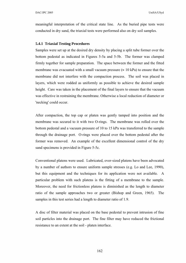
Samples were set up at the desired dry density by placing a split tube former over the

bottom pedestal as indicated in Figures 5-5a and 5-5b. The former was clamped

firmly together for sample preparation. The space between the former and the fitted

membrane was evacuated with a small vacuum pressure (≈ 10 kPa) to ensure that the

membrane did not interfere with the compaction process. The soil was placed in

layers, which were rodded as uniformly as possible to achieve the desired sample

height. Care was taken in the placement of the final layers to ensure that the vacuum

was effective in restraining the membrane. Otherwise a local reduction of diameter or

'necking' could occur.

After compaction, the top cap or platen was gently tamped into position and the

membrane was secured to it with two O-rings. The membrane was rolled over the

bottom pedestal and a vacuum pressure of 10 to 15 kPa was transferred to the sample

through the drainage port. O-rings were placed over the bottom pedestal after the

former was removed. An example of the excellent dimensional control of the dry

sand specimens is provided in Figure 5-5c.

Conventional platens were used. Lubricated, over-sized platens have been advocated

by a number of authors to ensure uniform sample stresses (e.g. Lo and Lee, 1990),

but this equipment and the techniques for its application were not available. A

particular problem with such platens is the fitting of a membrane to the sample.

Moreover, the need for frictionless platens is diminished as the length to diameter

ratio of the sample approaches two or greater (Bishop and Green, 1965). The

samples in this test series had a length to diameter ratio of 1.9.

A disc of filter material was placed on the base pedestal to prevent intrusion of fine

soil particles into the drainage port. The fine filter may have reduced the frictional

resistance to an extent at the soil - platen interface.

162


The cell was then filled with water and a cell pressure slightly greater than the

temporary vacuum pressure was applied. The vacuum pressure was then removed

and the base drainage port was left open to allow release of air from the dry sample.

Minor settlement of the sample may have occurred during this set-up period as a

small, isotropic pre-consolidation pressure of a maximum of 30 kPa was applied to

the sample for a short period as the sample former and vacuum pressure were

removed.

Care was taken to establish the initial density of each specimen. The diameter of the

sample was taken to be the diameter of the split former less two thicknesses of the

rubber membrane. A membrane thickness of 0.35mm was found to be the practical

minimum thickness for this soil to ensure leaks did not occur at the large sample

strains attained in the tests. The height of the sample was measured with the top

platen in position. All samples were approximately 100 mm in diameter and 190 mm

long. The mass of the sample was established by weighing a chosen mass of the dry

soil used to form the sample, and then deducting the mass of soil remaining after

preparation of the sample. The final sample mass was measured by carefully

collecting the soil at the end of the test. Inevitably, some grains of the dry sand were

lost in this final operation.

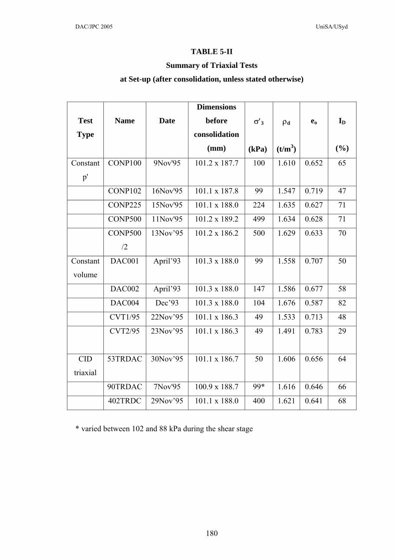
Table 5-II provides a summary of the 13 tests that were conducted and the initial

sample parameters. Most samples were prepared to a medium dense state with

density indices in the range from 50 to 70% after the initial isotropic consolidation

stage. Two constant volume test samples, DAC004 and CVT2/95, had density

indices outside this range and were relatively dense and loose, respectively.

All samples were isotropically consolidated before commencing the main test by

ramping the cell pressure at a rate of 2.5kPa / minute. The initial settlement due to

consolidation was relatively small and was assumed to be isotropic.

During testing, volume changes were estimated from cell fluid volume changes,

which were measured by a GDS hydraulic ram system. Volumes were corrected for

cell volume changes (expansion or contraction) with cell pressure. Corrections were

also made for the penetration of the loading ram. The dependence of cell volume on

163


cell pressure was established by placing a steel cylinder of similar dimensions to a

soil sample in the cell, applying a cell pressure and recording the change in volume

of the cell fluid on the GDS device. The cell fluid volume stabilised after

approximately ten minutes, depending on the level of cell pressure increment. De-

aired, de-mineralized water was used for the cell fluid. It was found that some air

still existed in the water after 'de-airing' and it was essential to carry out a number of

cell calibration runs before the calibration settled down. With air in the system, cell

volume changes are greater than the apparent measurement, as air is forced into

solution.

Axial strains were measured electronically outside the cell, while axial load was

measured inside the cell. Calibrations of both displacement and load transducers

were performed prior to each test series.

The maximum axial strain rate in all the tests was 0.05 mm/minute. Wherever

possible, axial strains were taken above 25%.

Sample length and volume changes were used to derive the average area of the

sample during testing to determine the deviator stress, q.

5.5 RESULTS OF THE TRIAXIAL TESTS

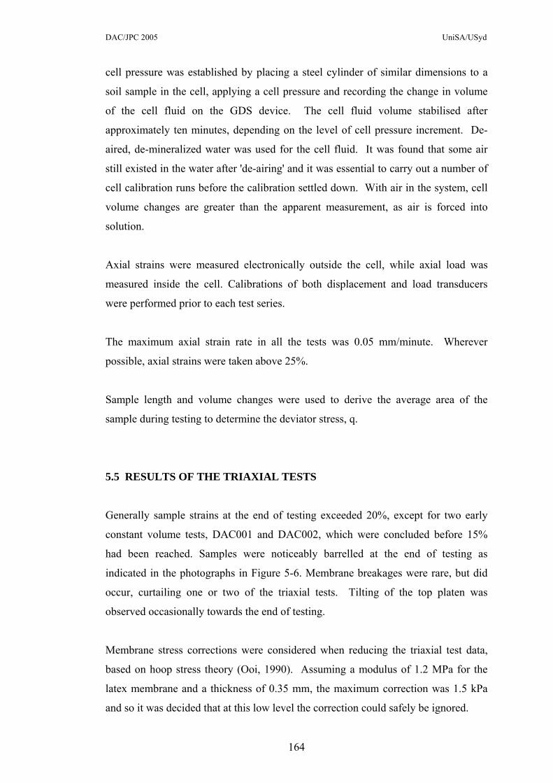
Generally sample strains at the end of testing exceeded 20%, except for two early

constant volume tests, DAC001 and DAC002, which were concluded before 15%

had been reached. Samples were noticeably barrelled at the end of testing as

indicated in the photographs in Figure 5-6. Membrane breakages were rare, but did

occur, curtailing one or two of the triaxial tests. Tilting of the top platen was

observed occasionally towards the end of testing.

Membrane stress corrections were considered when reducing the triaxial test data,

based on hoop stress theory (Ooi, 1990). Assuming a modulus of 1.2 MPa for the

latex membrane and a thickness of 0.35 mm, the maximum correction was 1.5 kPa

and so it was decided that at this low level the correction could safely be ignored.

164


The following section provides data on the sand relating to the properties:

• Initial compressibility under isotropic loading (consolidation stage)

• Soil stiffness

• Post-peak behaviour

• Shear strength

• Constant volume shear strength

• Dilation

A summary of the major findings is given at the end of the Chapter.

5.5.1 Soil Compressibility in the Isotropic Consolidation Stage

The isotropic consolidation stage of the triaxial tests provided information on the

initial compressibility of the soil over a range of densities and mean stresses (refer

Figure 5-7). Four of the triaxial tests were not included in the plot, because of the

small change of the cell confining pressure in the initial consolidation phase for these

tests.

A compression index could be discerned for each of the samples, which was

reasonably constant over a designated mean stress range. In some cases where the

stress levels were high, two indices have been reported for the one test,

corresponding to different stress ranges. The initial compression indices, C, for the

samples have been presented in Table 5-III, with C being defined as:

)p∆(ln

∆eC′

−= 5-1

An examination of the data in Table 5-III revealed that the compressibility increased

with the average of the mean stress range and was little influenced by the variations

in density index of the samples.

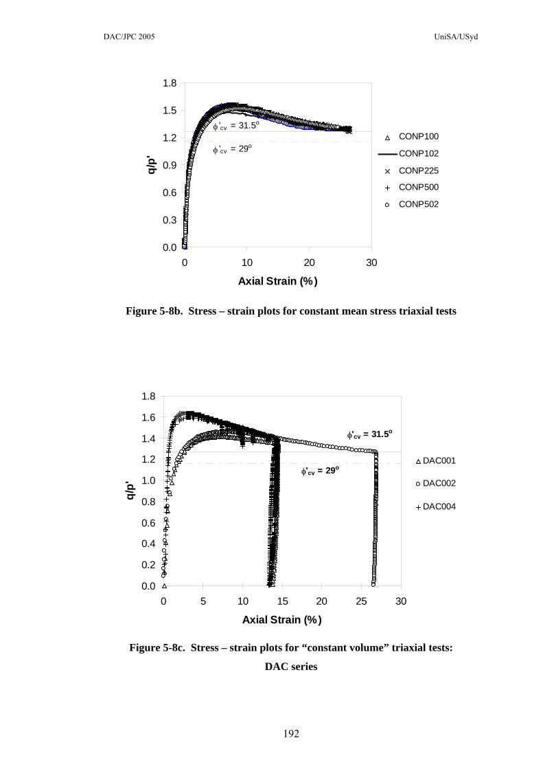
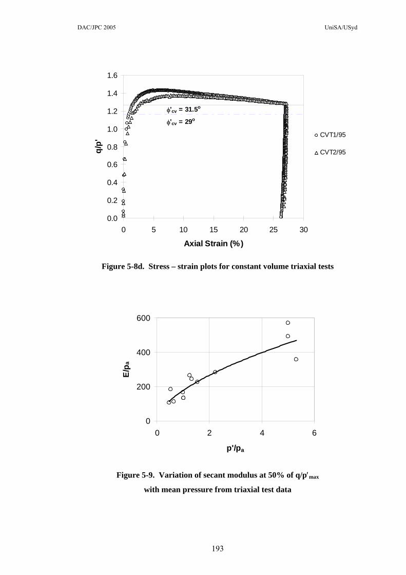
5.5.2 Stress-Strain Data

Figure 5-8 provides the relationships measured in the experiments between the stress

ratio, q/p′, and axial strain for the various test series. As the numerical modelling

required a convenient form with which to express the stiffness of the soil and its

variation with stress, the triaxial tests were interpreted to give moduli, E. For

165


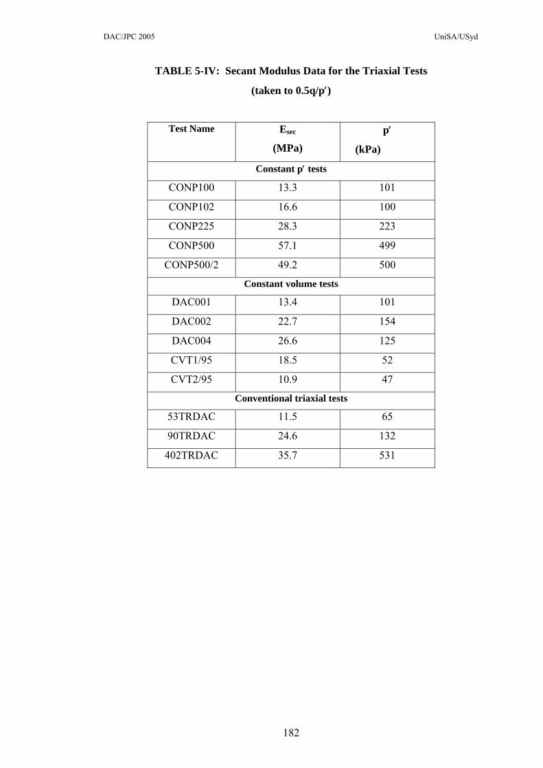
simplicity, it was decided to determine secant values rather than a tangent moduli.

Tangent moduli can be determined from secant values as expained later. The stress

level at which the secant modulus was determined was 0.5q/p′max.

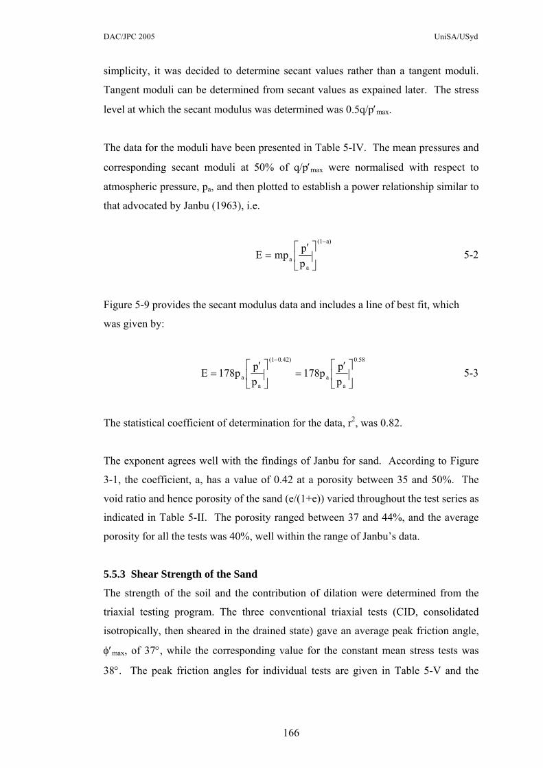
The data for the moduli have been presented in Table 5-IV. The mean pressures and

corresponding secant moduli at 50% of q/p′max were normalised with respect to

atmospheric pressure, pa, and then plotted to establish a power relationship similar to

that advocated by Janbu (1963), i.e.

a)(1

aa p

pmpE−

⎥⎦

⎤⎢⎣

⎡ ′= 5-2

Figure 5-9 provides the secant modulus data and includes a line of best fit, which

was given by:

0.58

aa

0.42)(1

aa p

p178ppp178pE ⎥

⎦

⎤⎢⎣

⎡ ′=⎥

⎦

⎤⎢⎣

⎡ ′=

−

5-3

The statistical coefficient of determination for the data, r2, was 0.82.

The exponent agrees well with the findings of Janbu for sand. According to Figure

3-1, the coefficient, a, has a value of 0.42 at a porosity between 35 and 50%. The

void ratio and hence porosity of the sand (e/(1+e)) varied throughout the test series as

indicated in Table 5-II. The porosity ranged between 37 and 44%, and the average

porosity for all the tests was 40%, well within the range of Janbu’s data.

5.5.3 Shear Strength of the Sand

The strength of the soil and the contribution of dilation were determined from the

triaxial testing program. The three conventional triaxial tests (CID, consolidated

isotropically, then sheared in the drained state) gave an average peak friction angle,

φ′max, of 37°, while the corresponding value for the constant mean stress tests was

38°. The peak friction angles for individual tests are given in Table 5-V and the

166


variation of this strength parameter with initial sample density over all the tests is

given in Figure 5-10.

The peak friction angle increased almost linearly with density index. The

relationship could be approximated by the expression;

φ′max = 0.104ID + 30.6 5-4

where, φ′max is in degrees and ID is in %.

The critical state strength (φ′cv) was evaluated from the stress conditions at the end of

testing. The accuracy of such an approach depends on whether or not critical state

had been reached. In section B.1 of Appendix B, the rate of volume strain with axial

strain has been imposed on the stress-strain plots for each of the tests. It can be seen

that the rate of volume strain had slowed by the end of each test, but it could not be

said that it had stopped, despite the large shear strains developed in the tests.

Therefore the estimate of φ′cv will be on the high side.

Furthermore the accuracy of this estimate will depend on whether a general failure

had developed throughout each sample or shear banding had dominated the soil

behaviour. In the latter case, the critical state may only prevail in the locality of the

shear band.

The data have been plotted in Figure 5-11 and it can be seen that the data are

bounded by values of 33° and 31.5°. One point (DAC004) has been omitted from

this Figure for the purpose of clarity, as the stresses associated with it were much

higher than for any other test. DAC004 plotted almost on the 33° line. The stress-

strain (q/p against εa) plots for each test series in Figure 5-8 have had two potential

values of the critical state stress ratio, Μ, imposed upon them for φ′cv values of 31.5°

and 29°. The corresponding values of Μ are 1.27 and 1.16. The latter estimate will

be discussed in the next section. It is evident from Figure 5-8 that a value of φ′ of

31.5° forms a reasonable lower bound to the test data.

167


Referring to equation 5-4, a further estimate of φ′cv is provide by the constant of 30.6,

which is equivalent to the friction angle at a density index of zero in degrees. This

value is almost one degree less than the value derived from the end of test data.

However this value relies on extrapolation of an assumed linear relationship between

φ′max and ID.

5.5.4 The Critical State Line

By plotting the end points of the three series of tests on a plot of void ratio, e, against

the natural logarithm of the effective mean stress, ln p′, an approximation to the

critical state line may be made, assuming that critical state has been reached. The

constant volume tests are presented in Figure 5-12. It is clear from this plot that the

first three tests were not truly constant volume tests; a small error in the algorithm for

volume control was found subsequently and corrected. Furthermore, tests DAC001

and DAC004 were ended at relatively low levels of axial strain and were unlikely to

have been close to critical state.

A suggested critical state line is indicated on the Figure, which is defined by an

intercept on the void ratio axis, Γ, of 1.07 at a reference effective mean stress, p′, of 1

kPa, and a gradient, λ, of 0.055. The end point for DAC004 is furthest removed

from the line, which is most probably due to the early termination of the test and the

high level of mean stress reached in this test (approximately 1400 kPa). Some

particle breakage may have occurred at this stress level, which would shift the

critical state line, increasing the magnitude of its gradient, as observed by Been,

Jefferies, and Hachey (1991) and Ajalloeian and Yu (1996).

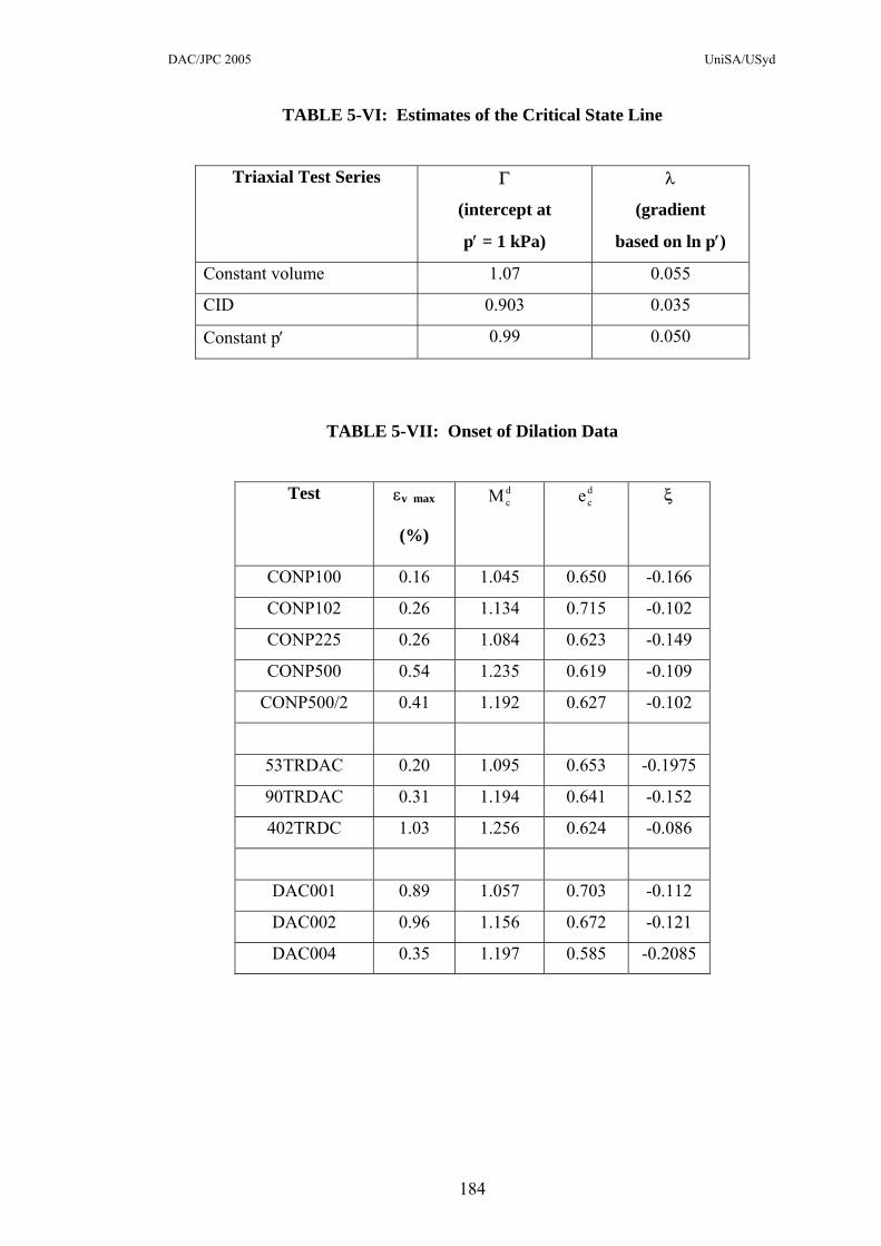
The two remaining test series have been plotted similarly in Figures 5-13 and 5-14,

and a critical state line has been judged for each series. A statistical fit was not

deemed appropriate for the data. The variation of the critical state line parameters

for the three test series is provided in Table 5-VII. The three conventional triaxial

tests provided a state line with a relatively low gradient, indicating less compressible

soil.

168


End points for all tests have been plotted in Figure 5-15 and the estimates of the CSL

have been drawn over the data. It can be seen that the “constant volume” tests

generally reached higher void ratios by the conclusion of testing for a given stress

level than either the CID or constant mean stress tests. The latter two series of tests

reached similar levels of void ratio and a single critical state line defined by Γ = 0.99

and λ = 0.05 would seem reasonable for these tests.

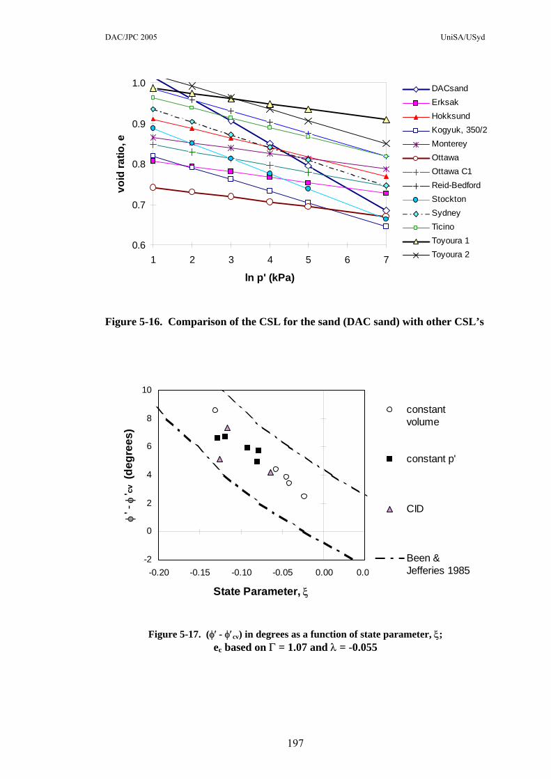
The adopted critical state line for the sand from the constant volume tests, has been

compared with others reported in the literature in Figure 5-16 (the adopted CSL is

denoted as “DAC sand”). The adopted CSL was defined by Γ of 1.07 and λ of

0.055. Both the gradient and the intercept at the reference pressure of 1 kPa were

outside the bounds of the published data; the gradient was relatively high, indicating

significantly more compressible sand. The intercept was similar to that for Reid-

Bedford sand, however the gradients differed by a factor of 2. Reid Bedford sand

has been described as sub-angular, while the sand in the current study was angular.

The difference in the maximum and minimum void ratios was greater (16%) than

Reid Bedford sand, and the uniformity coefficient of 2.6 compared with a value of

1.6, indicating that “DAC sand” was more poorly graded.

Hokksund sand has been reported as sub-angular sand, with similar properties to

DAC sand. The major difference was the basic particle size (D10 = 0.21, while for

DAC sand it was 0.16), which may be responsible for the relatively low

compressibility of the soil.

Knowing the critical state line, which as previously stated was based on the CSL

from the constant volume tests, and adopting a critical state strength of φ′cv of 31.5°,

the difference between the peak and critical state friction angles may be plotted

against the state parameter at (q/p′)max. The strength and dilation data from Table 5-

V were used for this Figure. The data have been plotted in Figures 5-17 and 5-18.

The data fit centrally within the bounds proposed by Been and Jefferies in 1985

(refer Figures 3-16 and 5-17). If either the CSL from the CID or constant mean

stress tests are applied, the data points tend to plot on the upper bound line proposed

169


by Been and Jefferies. By definition, a soil at critical state has a state parameter of

zero and φ′max should equal φ′cv. Therefore sands would be expected to pass through

the origin, close to the lower bound proposed by Been and Jefferies. The data in

Figure 5-17 indicate however, that a difference in the friction angles of almost 2°

could be expected at the critical state. The other two experimentally derived CSL’s

would suggest twice this value and are therefore considered to be less reliable. The

offset at a state parameter of zero may in part be due to overestimation of the critical

state strength.

The data in Figure 5-17 has been re-plotted in Figure 5-18 to evaluate the coefficient,

A, in the expression;

(φ' - φcv') radians = A(e-ξ - 1) 5-5

For the sand in this study the line of best fit to the data was given by:

(φ' - φcv') radians = 0.66(e-ξ - 1) + 0.034 [r2 = 0.80] 5-6

Enforcing the statistical trend line through zero gave the expression:

(φ' - φcv') radians = 0.98(e-ξ - 1) [r2 = 0.58] 5-7

The two lines given by these equations have been superimposed on the data in Figure

5-18, the broken line corresponding to equation 5-6 and the solid line corresponding

to 5-7. It is evident that the relationship expressed by 5-7 is unsatisfactory, as it will

overestimate φ′ at low values of state parameter and underestimate at high values.

A much simpler expression could be adopted based on a linear relationship between

the strength difference and state parameter:

(φ' - φcv') degrees = -41.5ξ + 1.8 [r2 = 0.80] 5-8

Enforcing the statistical trend line through zero altered the expression to:

170


(φ' - φcv') degrees = -59.6ξ [r2 = 0.62] 5-9

Alternatively, a parabolic relationship may better express the apparent non-linear link

between (φ′- φ′cv) and state parameter:

(φ′- φ′cv) degrees = -331ξ2 - 96.8ξ [r2 = 0.80] 5-10

This non-linear equation has the advantages that it enforces zero dilation once the

state parameter increases to zero and follows the data satisfactorily for this sand.

However the fit for the parabola is no better statistically than that for the linear

relationship of equation 5-8. The parabolic equation suggests that dilation may slow

at low values of state parameter. This feature of the correlation appears to be at odds

with the findings of Been and Jefferies.

All the expressions based on state parameter, which are represented by equations 5-8,

9 and 10, are compared with the data in Figure 5-19. The statistical fit is

significantly weakened by enforcing the critical state strength at critical state, or a

value of state parameter of zero. Equation 5-9 would appear to be the most

acceptable expression, both theoretically and experimentally for the range of state

parameters encountered in the laboratory test series, although it is not a statistically

strong relationship.

5.5.5 Dilational Behaviour of the Sand

As discussed in Chapter 3, Bolton (1986) defined dilation in terms of total strains,

i.e. equation 3-24:

1

vB dε

dεD −=

According to Bolton, a sample undergoing triaxial stresses would experience a

maximum dilation rate corresponding to its dilatancy index, IR. The dilatancy index

is a function of the effective mean stress and the density index of the soil.

171


The density index of the sand at peak strength provided values of IR, which gave

better correlations with soil parameters than the initial density index at set-up of the

soil sample. All values of Bolton’s dilatancy index subsequently referred to in this

thesis have been calculated using the density index at peak strength.

It was discovered that Bolton’s estimate of maximum dilation was reasonable

provided the material constant, Q, was 9, not 10 as in Bolton’s original formulation

(equation 3-26), although he had anticipated lower values of Q for weaker grained

soils. Material constant, R, remained at unity. Therefore the sand in this study has a

dilation index best expressed by:

1)pln(9II DR −′−= 5-11

The maximum value of Bolton’s dilation for each of the triaxial tests has been

plotted in Figure 5-20 against IR, as determined by eqn 5-11. The density index at

maximum stress ratio has been adopted to generate values of IR. In the same Figure,

the maximum dilation has been plotted against state parameter at maximum stress

ratio. It would appear that state parameter is a slightly better indicator of dilation.

The similarity of the two plots suggested a strong relationship between state

parameter and dilatancy index, as one would expect with both indices being

functions of effective mean stress and void ratio. When plotted against one another

(Figure 5-21), it was found that dilation index was reliably given by:

10.7ξIR −= [r2 = 0.94] 5-12

This equation is represented by the trend line to the data in Figure 5-21. A slightly

better correlation is possible if a zero offset is accepted.

Bolton’s recommendation of DBmax = 0.3IR may then be replaced by:

3.20ξD maxB −= 5-13

172


This relationship appears as a straight line on the plot of dilation against state

parameter in Figure 5-20.

Bolton (1986) suggested that the maximum dilation under triaxial conditions may be

found from the dilatancy index according to equation 3-28:

(φ′max - φ′cv) = 3IR°

However it was found that with the value of Q adopted in this study and the

application of the density index at peak strength to derive IR, the above equation

significantly underestimated dilation. The plot in Figure 5-22 of the difference in the

two angles of friction against dilatancy index revealed that at least 6IR would be

needed to approach the levels of dilation realised in this test series. Combining

equations 5-9 and 5-12 provided the following outcome;

(φ′max - φ′cv) = 5.57IR° 5-14

Interestingly, Bolton recommended a value of 5IR° for plane strain conditions. So it

may be concluded that for this sand, Bolton’s equation for plane strain is a better

approximation to the triaxial compression data than his recommendation for triaxial

strain.

The curved line in Figure 5-22 has been produced by combining equations 5-10 and

5-12, resulting in a non-linear relationship between the friction angle difference and

Bolton’s dilatancy index, i.e.:

(φ′max - φ′cv) = -2.89IR2 + 9.05IR 5-15

The Davis flow rule, which was extended to triaxial compression of frictional soils

by Carter, Booker and Yeung (1986), was applied to the test data to derive estimates

of the maximum dilation angle, Ψmax. This estimate was then plotted against the

experimental data of (φ′max - φ′cv), Bolton’s index, IR and state parameter, ξ, in

Figures 5-23, 24 and 25, respectively.

173


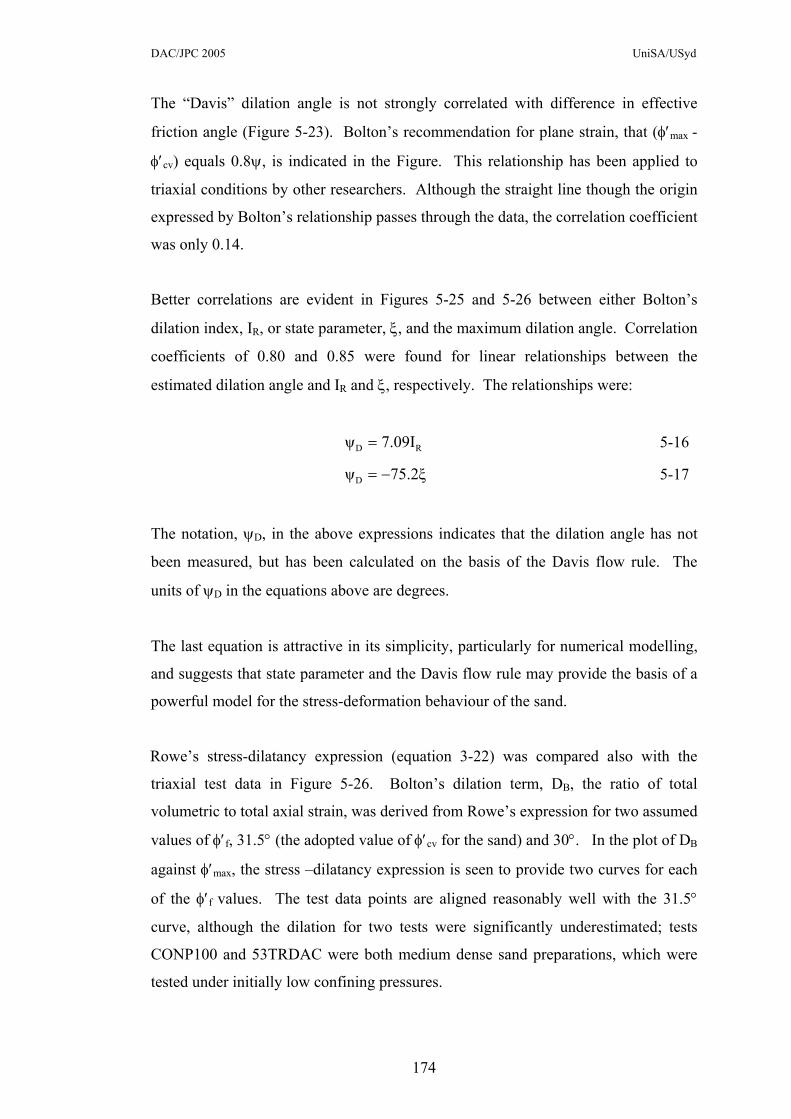
The “Davis” dilation angle is not strongly correlated with difference in effective

friction angle (Figure 5-23). Bolton’s recommendation for plane strain, that (φ′max -

φ′cv) equals 0.8ψ, is indicated in the Figure. This relationship has been applied to

triaxial conditions by other researchers. Although the straight line though the origin

expressed by Bolton’s relationship passes through the data, the correlation coefficient

was only 0.14.

Better correlations are evident in Figures 5-25 and 5-26 between either Bolton’s

dilation index, IR, or state parameter, ξ, and the maximum dilation angle. Correlation

coefficients of 0.80 and 0.85 were found for linear relationships between the

estimated dilation angle and IR and ξ, respectively. The relationships were:

RD 7.09Iψ = 5-16

75.2ξψD −= 5-17

The notation, ψD, in the above expressions indicates that the dilation angle has not

been measured, but has been calculated on the basis of the Davis flow rule. The

units of ψD in the equations above are degrees.

The last equation is attractive in its simplicity, particularly for numerical modelling,

and suggests that state parameter and the Davis flow rule may provide the basis of a

powerful model for the stress-deformation behaviour of the sand.

Rowe’s stress-dilatancy expression (equation 3-22) was compared also with the

triaxial test data in Figure 5-26. Bolton’s dilation term, DB, the ratio of total

volumetric to total axial strain, was derived from Rowe’s expression for two assumed

values of φ′f, 31.5° (the adopted value of φ′cv for the sand) and 30°. In the plot of DB

against φ′max, the stress –dilatancy expression is seen to provide two curves for each

of the φ′f values. The test data points are aligned reasonably well with the 31.5°

curve, although the dilation for two tests were significantly underestimated; tests

CONP100 and 53TRDAC were both medium dense sand preparations, which were

tested under initially low confining pressures.

174


Manzari and Dafalias (1997) suggested that the stress ratio at the onset of dilation,

was needed to adequately predict dilation (refer Chapter 3, equation 3-46). The

authors contended that was a function of state parameter (refer equation 3-47),

with

dcΜ

dcΜ

( )dcc ΜΜ − being directly proportional to state prameter, ξ.

Data concerning the onset of dilation from the triaxial tests has been summarised in

Table 5-VII. is the void ratio at the onset of dilation. The state parameter was

evaluated for this void ratio and the effective mean stress by adopting Γ of 1.07 and

λ of 0.055.

dce

Combining the data in Tables 5-V and 5-VII leads to the plots of ( )dcc ΜΜ − against

state parameter in Figure 5-27, and dilation against ( )maxdc ηΜ − in Figure 5-28. Mc

was based on a φ′cv value of 31.5°. The dilation in Figure 5-28 is the maximum

“total” dilation, defined by the ratio of total volumetric strain to total shear strain.

It is evident that there is not a strong correlation between ( )dcc ΜΜ − and state

parameter, thereby diminishing the usefulness of Manzari and Dafalias’ model for

this sand. However their flow rule is supported reasonably well by the test data in

Figure 5-28, despite the use of total strains to define dilation. Again the correlation

as illustrated by the dashed trendline is weak (r2 = -0.2), caused largely by four

outlying points. The trendline in the Figure has a gradient of 0.73, giving a value of

0.90 for the Manzari and Dafalias’ coefficient, A, in equation 3-46.

175


5.6 SUMMARY OF THE CHAPTER

The sand in the study was a poorly graded sand formed by crushing of quartzite.

Consequently the sand grains were angular and mica and feldspar particles were

present.

Three series of triaxial tests were performed on the dry sand, which had been

prepared at a range of densities (ID approximately 30 to 80%). The tests included

consolidated isotropically, conventional drained triaxial tests (CID), constant volume

and constant mean stress tests. A major aim of the triaxial tests was to induce large

axial strains so that information about the critical state of the sand could be obtained.

The major findings of this limited experimental study were;

(i) The initial compressibility of the sand under isotropic loading was low.

(ii) Shearing of the soil to large strain produced strain softening and associated

dilation.

(iii) The secant modulus of the soil at 50% peak stress ratio could be reasonably

well represented by a power relationship with effective mean pressure as

proposed by Janbu (1963) and, significantly, the coefficients in the

relationship agreed with Janbu’s recommended values.

(iv) The peak shear strength of the sand in the various tests was found to vary in

direct proportion to the initial sample density index.

(v) The critical state shear strength, φ′cv, was estimated to be 31.5°.

(vi) The critical state line varied slightly between the different types of tests, with

the constant volume tests providing a “higher” CSL, defined by values of Γ

of 1.07 and λ of 0.055. This was the chosen CSL as it gave a lower positive

value of (φ′-φ′cv) at a state parameter of zero than the alternatives.

(vii) The parameter, A, (Collins, Pender and Yan, 1992) needed to define the

relationship between (φ' - φcv') and state parameter, ξ, was determined to be

0.98. The fit to the experimental data was not strong and would be

substantially improved if φ' was allowed to be slightly greater than φcv' at a

value of state parameter of zero. However such an assumption is

theoretically untenable.

176


(viii) A simpler and slightly better expression was derived for the range of state

parameters encountered in the triaxial tests, i.e. (φ' - φcv') degrees = -59.6ξ.

(ix) Bolton’s dilatancy index (1986) was found to be proportional to the

magnitude of the state parameter, i.e. IR = -10.7ξ. Accordingly, the

maximum dilation, expressed in terms of total volumetric strain to total axial

strain, was directly related to state parameter by the equation, DB max = -3.2ξ.

(x) Bolton’s dilatancy index was formulated with Q being equal to 9, rather than

10. Bolton had anticipated that lower values of Q might be appropriate for

more angular sands.

(xi) Bolton’s recommendation of (φ′max - φ′cv) = 3IR° for triaxial stress state was

found to underestimate the difference in shear strength angles by at least

50%. Bolton’s equation for plane strain, (φ′max - φ′cv) = 0.8Ψ, was a better

approximation to the triaxial compression data.

(xii) Davis’ flow rule (1969) for triaxial conditions, when applied to the

experimental data, yielded estimates of dilation angle (ψD) which were found

to correlate well against both Bolton’s dilation index and state parameter.

The state parameter correlation was found to be slightly stronger. Dilation

angle in degrees can be approximated by multiplying ξ by a factor of –75.

(xiii) The triaxial test data agreed generally with Rowe’s (1962) stress-dilatancy

expression, and the assumption that φ′f is equal to φ′cv.

(xiv) The flow rule of Manzari and Dafalias (1997), which is based on the stress

ratio at the onset of dilation, was reasonably supported by the triaxial data for

the sand.

From the triaxial test data reviewed in this Chapter, material constants and other

parameters have been chosen for the constitutive model of the soil, placed around

and above the buried pipe. A constitutive model of the soil is essential to the finite

element analysis of the response of the soil-pipe system to external loading. In

particular, the critical state shear strength and CSL were chosen, and the relationship

linking the difference in effective angle of friction to the state parameter, i.e.,

(φ' - φcv') radians = 0.98(e-ξ - 1), was adopted. Both Bolton’s equation for dilation of

sand in plane strain and Davis’ flow rule were incorporated into the soil model.

177


The development of the constitutive model is provided in Chapter 6, with validation

through comparison of finite element analyses (FEA) with the results of plate bearing

tests of the sand contained in a drum. Chapters 7 and 8 subsequently explore the

FEA of the the buried pipes in two and three dimensions.

5.7 REFERENCES TO CHAPTER 5

Bishop, A. W. and Green, G. E. (1965). The Influence of End Restraint on the

Compression Strength of a Cohesionless Soil. Geotechnique, V15, No. 3, pp 243-

266.

Lo, S.-C. R. and Lee, I. K. (1990). Response of Granular Soil along Constant Stress

Increment Ratio Path. ASCE, J. of Geotechnical Engineering, V116, No. 3, March,

pp 355-376.

Ooi, J.Y. (1990). Bulk Solids Behaviour and Silo Wall Pressures. PhD thesis,

University of Sydney, School of Civil and Mining Engineering.

178


TABLE 5-I. Particle Size Analysis

Particle sizes (mm) Particle size

analysis indices

D10 D30

D60 Cu Cc

0.16 0.245 0.41 2.6 0.92

Dn = n % of particles are smaller than this size

Cu = uniformity coefficient

Cc = the coefficient of curvature

179


TABLE 5-II

Summary of Triaxial Tests

at Set-up (after consolidation, unless stated otherwise)

Test

Type

Name

Date

Dimensions

before

consolidation

(mm)

σ′3

(kPa)

ρd

(t/m3)

eo

ID

(%)

Constant

p'

CONP100 9Nov'95 101.2 x 187.7 100 1.610 0.652 65

CONP102 16Nov'95 101.1 x 187.8 99 1.547 0.719 47

CONP225 15Nov'95 101.1 x 188.0 224 1.635 0.627 71

CONP500 11Nov'95 101.2 x 189.2 499 1.634 0.628 71

CONP500

/2

13Nov’95 101.2 x 186.2 500 1.629 0.633 70

Constant

volume

DAC001 April’93 101.3 x 188.0 99 1.558 0.707 50

DAC002 April’93 101.3 x 188.0 147 1.586 0.677 58

DAC004 Dec’93 101.3 x 188.0 104 1.676 0.587 82

CVT1/95 22Nov’95 101.1 x 186.3 49 1.533 0.713 48

CVT2/95

23Nov’95 101.1 x 186.3 49 1.491 0.783 29

CID

triaxial

53TRDAC 30Nov’95

101.1 x 186.7 50 1.606 0.656 64

90TRDAC 7Nov'95 100.9 x 188.7 99* 1.616 0.646 66

402TRDC 29Nov’95 101.1 x 188.0 400 1.621 0.641 68

* varied between 102 and 88 kPa during the shear stage

180


TABLE 5-III: Compression Index for the Isotropic Consolidation Stage

Test Name C

p′ range

(kPa)

Constant p′ tests

CONP100 0.008 43-100

CONP102 0.012 40-100

CONP225 0.011 65-225

CONP500 0.008

0.014

40-148

148-495

CONP500/2 0.009

0.013

35-165

165-500

Constant volume tests

DAC001 0.007 32-103

DAC002 0.007 40-135

CVT2/95 0.006 18-43

Conventional triaxial tests

90TRDAC 0.007 47-100

402TRDAC 0.013 100-400

181


TABLE 5-IV: Secant Modulus Data for the Triaxial Tests

(taken to 0.5q/p′)

Test Name Esec

(MPa)

p′

(kPa)

Constant p′ tests

CONP100 13.3 101

CONP102 16.6 100

CONP225 28.3 223

CONP500 57.1 499

CONP500/2 49.2 500

Constant volume tests

DAC001 13.4 101

DAC002 22.7 154

DAC004 26.6 125

CVT1/95 18.5 52

CVT2/95 10.9 47

Conventional triaxial tests

53TRDAC 11.5 65

90TRDAC 24.6 132

402TRDAC 35.7 531

182


TABLE 5-V: Strength and Dilation Data

Void ratio, e, at:

Test

Maxm.

Strain

εa max

(%)

p′max

(kPa)

q/p′max

φ′max

(°) q/p′ max εa max

DTmax

CONP100 25.8 99.5 1.55 38.1 0.689 0.792 -0.386

CONP102 26.6 100.1 1.48 36.4 0.736 0.806 -0.237

CONP225 26.5 222.7 1.56 38.2 0.654 0.739 -0.310

CONP500 26.3# 500.0 1.52 37.4 0.636 0.708 -0.246

CONP500/2 19.9∗ 500.8 1.51 37.2 0.649 0.685 -0.256

DAC001 14.5 304.5 1.41 34.9 0.714 0.723 -0.112

DAC002 26.9 400.5 1.45 35.9 0.683 0.701 -0.100

DAC004 14.4 491.9 1.64 40.1 0.598 0.633 -0.295

CVT1/95 26.3 289.2 1.43 35.3 0.713 0.713 0.000

CVT2/95 26.8 119.9 1.37 34 0.783 0.783 0.000

53TRDAC 27.9 101.4 1.49 36.6 0.690 0.745 -0.373

90TRDAC 24.5 188.9 1.59 38.9 0.665 0.722 -0.367

402TRDAC 26.8 781.8 1.48 36.3 0.640 0.675 -0.197

# minor membrane leak ∗ membrane leakage after this strain level

183


TABLE 5-VI: Estimates of the Critical State Line

Triaxial Test Series Γ

(intercept at

p′ = 1 kPa)

λ

(gradient

based on ln p′)

Constant volume 1.07 0.055

CID 0.903 0.035

Constant p′ 0.99 0.050

TABLE 5-VII: Onset of Dilation Data

Test εv max

(%)

dcΜ d

ce ξ

CONP100 0.16 1.045 0.650 -0.166

CONP102 0.26 1.134 0.715 -0.102

CONP225 0.26 1.084 0.623 -0.149

CONP500 0.54 1.235 0.619 -0.109

CONP500/2 0.41 1.192 0.627 -0.102

53TRDAC 0.20 1.095 0.653 -0.1975

90TRDAC 0.31 1.194 0.641 -0.152

402TRDC 1.03 1.256 0.624 -0.086

DAC001 0.89 1.057 0.703 -0.112

DAC002 0.96 1.156 0.672 -0.121

DAC004 0.35 1.197 0.585 -0.2085

184


0

20

40

60

80

100

0.0 0.1 1.0 10.0

Particle Size (mm)

Perc

ent P

assi

ng

Figure 5-1. Average particle size distributions for two triaxial test specimens

(before testing)

0

20

40

60

80

100

0.0 0.1 1.0 10.0Particle Size (mm)

Perc

ent P

assi

ng

DAC001, after testing DAC004, after testing Average before testing

Figure 5-2. Particle size distributions for two triaxial test specimens

after testing

185


Figure 5-3. Scanning Electron Microscope images of the sand

186


0

200

400

600

800

0 5 10 15 Settlement (mm)

App

lied

Pres

sure

(kPa

)

Figure 5-4. Plate loading test results for the sand confined in a drum

(ID ≈ 75%)

Membrane O ring

Vacuum portsSample former

Base Pedestal

Temporary support

Drainageport

Figure 5-5a. Cross sectional view of sample preparation

187


Figure 5-5b. Photograph of the split tube former ready

to receive the sand sample

Figure 5-5c. An example of a prepared sample of dry sand

188


Figure 5-6a. Specimen after a CID triaxial test (90TRDAC, σ3 = 99 kPa)

Figure 5-6b. Specimen after a constant pressure test (CONP225, p′ = 225 kPa)

189


Figure 5-6c. Specimen after a constant pressure test (CONP500, p′ = 499 kPa)

Figure 5-6d. Specimen after a constant volume test (CVT2/95)

190


0.60

0.65

0.70

0.75

0.80

2.5 3.5 4.5 5.5 6.5

ln p'

Void

Rat

io, e

DAC002

DAC001

CONP100

CONP500

CONP502

90TRDAC

402TRDAC

CVT2/95

CONP102

CONP225

Figure 5-7. Isotropic Consolidation Curves

0.0

0.3

0.6

0.9

1.2

1.5

1.8

0 5 10 15 20 25 30Axial Strain (%)

q/p'

50 kPa

99 kPa

400 kPa

φ'cv = 31.5o

φ'cv = 29o

σ'3

Figure 5-8a. Stress – strain plots for conventional (CID) triaxial tests

191


0.0

0.3

0.6

0.9

1.2

1.5

1.8

0 10 20 30

Axial Strain (%)

q/p'

CONP100

CONP102

CONP225

CONP500

CONP502

φ 'cv = 31.5o

φ 'cv = 29o

Figure 5-8b. Stress – strain plots for constant mean stress triaxial tests

0.0

0.2

0.4

0.6

0.8

1.0

1.2

1.4

1.6

1.8

0 5 10 15 20 25 30

Axial Strain (%)

q/p'

DAC001

DAC002

DAC004

φ'cv = 31.5o

φ'cv = 29o

Figure 5-8c. Stress – strain plots for “constant volume” triaxial tests:

DAC series

192


0.0

0.2

0.4

0.6

0.8

1.0

1.2

1.4

1.6

0 5 10 15 20 25 30

Axial Strain (%)

q/p'

CVT1/95

CVT2/95

φ'cv = 31.5o

φ'cv = 29o

Figure 5-8d. Stress – strain plots for constant volume triaxial tests

0

200

400

600

0 2 4 6

p'/pa

E/p a

Figure 5-9. Variation of secant modulus at 50% of q/p′max

with mean pressure from triaxial test data

193


34

36

38

40

42

0 50 100

Initial Density Index (%)

φ' max

(deg

rees

)

Constant p'

DAC series

Constant volume

CID

Figure 5-10. Relationship between peak friction angle

and initial density index of sample

0

200

400

600

800

1000

0 200 400 600 800

p' (kPa)

q (k

Pa)

constantvolume

constant p'

CID

φ 'cv = 33o φ 'cv = 31.5o

Figure 5-11. Critical state strength (φ′cv) estimated from stress state at

end of triaxial tests (DAC004 omitted)

194


0.5

0.6

0.7

0.8

0.9

2 3 4 5 6 7 8

ln p' (kPa)

DAC001

DAC002

DAC004

CVT1/95

CVT2/95

Figure 5-12. Mean stress excursions in the constant volume tests in

e – ln p′ space (circles indicate end points of tests)

0.5

0.6

0.7

0.8

3 4 5 6 7

ln p' (kPa)

Void

Rat

io, e

53TRDAC90TRDAC 402TRDAC

Figure 5-13. Mean stress excursions in the CID triaxial tests in e – ln p′ space

195


0.5

0.6

0.7

0.8

3 4 5 6 7

ln p' (kPa)

Void

Rat

io, e start of test (1)

end of test (1)

start of test (2)

end of test (2)

CONP100

CONP102

CONP225

CONP500

CONP502

Figure 5-14. Mean stress excursions in the constant mean stress tests

in e – ln p′ space

0.5

0.6

0.7

0.8

0.9

3 4 5 6 7 8

ln p'

Void

Rat

io, e

CID constant p' constant volume

Figure 5-15. Estimates of the CSL for each of the three triaxial test series

196


0.6

0.7

0.8

0.9

1.0

1 2 3 4 5 6 7

ln p' (kPa)

void

ratio

, e

DACsandErksakHokksundKogyuk, 350/2MontereyOttawaOttawa C1Reid-BedfordStocktonSydneyTicinoToyoura 1Toyoura 2

Figure 5-16. Comparison of the CSL for the sand (DAC sand) with other CSL’s

-2

0

2

4

6

8

10

-0.20 -0.15 -0.10 -0.05 0.00 0.05

State Parameter, ξ

φ' -

φ' cv

(de

gree

s)

constantvolume

constant p'

CID

Been &Jefferies 1985

Figure 5-17. (φ′ - φ′cv) in degrees as a function of state parameter, ξ; ec based on Γ = 1.07 and λ = -0.055

197


0.00

0.05

0.10

0.15

0.20

0.00 0.05 0.10 0.15

(e-ξ) - 1

φ' -

φ' cv

(rad

ians

)constantvolume

constant p'

CID

Figure 5-18. (φ′ - φ′cv) in radians as a function of state parameter;

data from Figure 5-17 (gradient of line = A = 0.98)

0

1

2

3

4

5

6

7

8

9

10

-0.15 -0.10 -0.05 0.00

State Parameter, ξ

( φ' -

φ' cv

) deg

rees

CID Constant p' Constant volume

(φ ' - φ 'cv) = -59.6ξ

(φ ' - φ 'cv) = -41.5ξ + 1.8

(φ ' - φ 'cv) = -331ξ2 -96.8ξ

Figure 5-19. Empirical expressions relating (φ′ - φ′cv) to state parameter

198


IR from Q = 9; R = 1

-0.5

-0.4

-0.3

-0.2

-0.1

0.0-2.0 -1.5 -1.0 -0.5 0.0 0.5 1.0 1.5 2.0

-DB

= ∆

εv /

∆ε1


STATE PARAMETER, ξ x 10 RELATIVE DILATANCY INDEX, IR

Bolton 1986, DB = 0.3IR

Figure 5-20. Bolton’s maximum dilation rate as a function

of both dilatancy index and state parameter

0

0.5

1

1.5

-1.5 -1 -0.5 0

State Parameter x10, 10ξ

Bol

ton'

s R

elat

ive

Dila

tanc

y In

dex,

I R

Figure 5-21. Bolton’s dilation index as a function of state parameter

199


0

2

4

6

8

10

0.0 0.5 1.0 1.5

Bolton's Relative Dilatancy Index, IR

( φ' -

φ' cv

)


φ ' - φ 'cv = 5.57IRo

Figure 5-22. Experimental data of (φ′- φ′cv) plotted against

Bolton’s dilation index

0

2

4

6

8

10

0 2 4 6 8 10 1

ψ max (degrees)

( φ' -

φ' cv

) (d

egre

es)

2


trend line, 0.44ψmax + 2.7

0.8ψmax

Figure 5-23. Experimental data of (φ′- φ′cv) plotted against

dilation angle estimated from Davis’ flow rule (1969)

200


0.0

0.5

1.0

1.5

0 2 4 6 8 10 12

ψ max (degrees)

IR


Figure 5-24. Experimental data of Bolton’s dilation index plotted against

dilation angle, estimated from Davis’ flow rule (1969)

-0.15

-0.10

-0.05

0.000 2 4 6 8 10 12

ψ max (degrees)

ξ


Figure 5-25. State parameter from triaxial tests plotted against

dilation angle, estimated from Davis’ flow rule (1969)

201


-0.5

-0.4

-0.3

-0.2

-0.1

0.032 34 36 38 40 42

φ 'max (o)

Dila

tion

rate

, DB

constant p' constant volume CID

φ 'f = 31.5o

φ 'f = 30o

Figure 5-26. Maximum total dilation (volumetric strain to axial strain) against

effective peak friction angle

0

0.1

0.2

0.3

-0.3-0.2-0.10

State Parameter, ξ

(Mc -

Md c)

constant p' CID constant volume

Figure 5-27. ( )dcc ΜΜ − against state parameter at the onset of dilation

202


-0.4

-0.3

-0.2

-0.1

0-0.6-0.4-0.20

(Mdc − ηmax)

Dila

tion,

DTm

ax

constant p' constant volume CID

Figure 5-28. Maximum total dilation (volumetric strain to shear strain)

against ( )maxdc ηΜ −

203

Documents

CHAPTER 5: METHODOLOGY - CHARACTERIZATION OF THE BACKFILL SOILses.library.usyd.edu.au/bitstream/2123/680/14/adt... · CHAPTER 5: CHARACTERIZATION OF THE BACKFILL SOIL ... The average