163

Chapter 5

EFFECT OF SAMPLING ON REAL OCULAR

ABERRATION MEASUREMENTS.

This chapter is based on the article by Llorente, L. et al.,”The effect of

sampling on real ocular aberration measurements”, Journal of the Optical

Society of America A 24, 2783- 2796 (2007). The co-authors of the study

are: Susana Marcos, Carlos Dorronsoro and Steve Burns. A preliminary

version of this work was presented as an oral paper (Llorente et al., 2004b)

at the II EOS Topical Meeting on Physiological Optics in Granada. The

contribution of the author to the study was the performance of the

experimental measurements, and data processing and analysis, as well as

statistical analysis of the experimental data and of the data from

simulations performed by Steve Burns.

5.1.- ABSTRACT

PURPOSE: To assess the performance of different sampling patterns

in the measurement of ocular aberrations and to find out whether there

was an optimum pattern to measure human ocular aberrations.

METHODS: Repeated measurements of ocular aberrations were

performed in 12 healthy non surgical human eyes, and 3 artificial eyes,

164

with a LRT using different sampling patterns (Hexagonal, Circular and

Rectangular with 19 to 177 samples, and three radial patterns with 49

samples coordinates corresponding to zeroes of the Albrecht, Jacobi, and

Legendre functions). Two different metrics based on the RMS of difference

maps (RMS_Diff) and the proportional change in the wave aberration

(W%) were used to compare wave aberration estimates as well as to

summarize results across eyes. Some statistical tests were also applied:

hierarchical cluster analysis (HCA) and Student’s t-test. Computer

simulations were also used to extend the results to “abnormal eyes”

(Keratoconic, post-LASIK and post-RK eyes).

RESULTS: In general, for both artificial and human eyes, the “worst”

patterns were those undersampled. Slight differences were found for the

artificial eye with different aberrations pattern, compared to the other

artificial eyes. Usually those patterns with greater number of samples gave

better results, although the spatial distribution of the samples also seemed

to play a role, for our measured, as well as our simulated “abnormal”

eyes. There was agreement between the results obtained from our metrics

and from the statistical tests.

CONCLUSIONS: Our metrics proved to be adequate to compare

aberration estimates across sampling patterns. There may be an interaction

between the aberration pattern of an eye and the ability of a sampling

pattern to reliably measure the aberrations. This implied that just

increasing the number of samples was not as effective as choosing a better

sampling pattern. In this fashion, moderate density sampling patterns

based on the zeroes of Albrecht cubature or hexagonal sampling

performed relatively well, being a good compromise between accuracy

and density. These conclusions were also applicable in human eyes, in

spite of the variability in the measurements masking the sampling effects

except for undersampling patterns. Finally, the numerical simulations

165

proved to be useful to assess a priori the performance of different sampling

patterns when measuring specific aberration patterns.

5.2.- INTRODUCTION

As previously described in Chapter 1, aberrometry techniques

currently used for human eyes consist on measuring ray aberrations at a

discrete number of sampling points, and then estimate the wave

aberration using modal, zonal or combined reconstruction methods

(Chapter 1, section 1.2.2). It is, therefore, crucial for these techniques to

find out which is the minimum number of samples necessary to fully

characterize the aberration pattern of the eye. This is a question under

debate in the clinical as well as the scientific community. The optimal

number of sampling points represents a trade-off between choosing a

number of samples large enough to accurately estimate the wave

aberration (see Chapter 1, section 1.2.5.3), and reducing the measuring and

processing time. In addition, the distribution of the samples throughout

the pupil of the eye may also play a role. In this chapter, the influence of

the number and distribution of samples used in the aberrations

measurement on the resulting estimated wave aberration will be studied.

To our knowledge, there has not been a systematic experimental

study investigating whether increasing the sampling density over a certain

number of samples provides significantly better accuracy in ocular

aberration measurements, or whether alternative sampling configurations

would be more efficient. There have been theoretical investigations of

sampling configuration from both analytical and numerical approaches

which are described below. However, the applicability to human eyes

should be ultimately tested experimentally.

Cubalchini (Cubalchini, 1979) was the first to study the modal

estimation of the wave aberration from derivative measurements using a

least squares method, concluding that the geometry and number of

166

samples affected the wavefront estimations and that the variance of higher

order Zernike terms could be minimised by sampling as far from the

centre of the aperture as possible and minimising the number of samples

used to estimate a fixed number of terms and to take the measurements.

In 1997, Rios et al. (1997) found analytically for Hartmann sensing

that the spatial distribution of the nodes of the Albrecht cubatures (Bará et

al., 1996) made them excellent candidates for modal wavefront

reconstruction in optical systems with a centrally obscured pupil. This

sampling scheme could also be a good candidate for ocular aberrations,

due to the circular geometry of the cubature scheme. In addition, as the

Zernike order increases (i.e., higher order aberrations), the area of the

pupil more affected by aberrations tends to be more peripheral (McLellan

et al., 2006, Applegate et al., 2002, Cubalchini, 1979), and therefore ocular

wavefront estimates would potentially benefit by a denser sampling of the

peripheral pupil.

He et al. (1998) used numerical simulations to test the robustness of

the fitting technique they used for their SRR (least-square fit to Zernike

coefficients) to the cross-coupling or modal aliasing (interaction between

orders) as well as the error due to the finite sampling aperture. They

found that the error could be minimized by extracting the coefficients

corresponding to the maximum complete order possible (considering the

number of samples), in agreement with Cubalchini (Cubalchini, 1979), and

by using a relatively large sampling aperture, which practically covered

the measured extent of the pupil. Although this large sampling aperture

introduced some error due to the use of the value of the derivatives at the

centre of the sampling apertures to perform the fitting, and the rectangular

pattern they used did not provide an adequate sampling for radial basis

functions, simulations confirmed that the overall effect was relatively

small.

167

In 2003, Burns et al. (2003) computationally studied the effect of

different sampling patterns on measurements of wavefront aberrations of

the eye, by implementing a complete model of the wavefront processing

used with a “typical” HS sensor and modal reconstruction. They also

analyzed the effect of using a point estimator for the derivative at the

centre of the aperture, versus using the average slope across the

subaperture, and found that the second decreased modal aliasing

somewhat, but made little practical difference for the eye models. Given

that the higher order aberrations tended to be small, the modal aliasing

they found was subsequently small. Finally, they found that non-regular

sampling schemes, such as cubatures, were more efficient than grid

sampling, when sampling noise was high.

Díaz-Santana et al (Diaz-Santana et al., 2005), and Soloviev and

Vdovin (2005) developed analytical models to test different sampling

patterns applied to ocular aberrometry and HS sensing in astronomy,

respectively. Díaz-Santana et al. (2005) developed an evaluation model

based on matrices that included as input parameters the number of

samples and their distribution (square, hexagonal, polar lattice), shape of

the subpupil, size and irradiance across the pupil (uniform irradiance vs.

Gaussian apodisation), regarding the sampling. The other input

parameters were the statistics of the aberrations in the population, the

sensor noise, and the estimator used to retrieve the aberrations from the

aberrometer raw data. According to their findings, no universal optimal

pattern exists, but the optimal pattern will depend, among others on the

specific aberrations pattern to be measured. Soloviev et al.’s model

(Soloviev and Vdovin, 2005) used a linear operator to describe the HS

sensing, including the effects of the lenslets array geometry and the

demodulation algorithm (modal wavefront reconstruction). When

applying this to different sampling configurations, using the Kolmogorov

statistics as a model of the incoming wavefront, they found that their

pattern with 61 randomly spatially distributed samples gave better results

168

than the regular hexagonal pattern with 91 samples of the same sub-

aperture size (radius=1/11 times the exit pupil diameter), which covered

completely the extent of the pupil in the case of the 91-sample pattern. In

these theoretical models, an appropriate statistical input was crucial so

that their predictions can be generalized in the population. McLellan et al.

found (McLellan et al., 2006) that high order aberration terms show

particular relationships (i.e. positive interactions that increase the MTF

over other potential combinations), suggesting that general statistical

models should include these relationships in order to describe real

aberrations.

In this study, LRT2 was used to measure wave aberrations in human

eyes, with different sampling patterns and densities. Hexagonal and

Rectangular configurations were chosen because they are the most

commonly used. Different radially symmetric geometries were also used

to test whether these patterns were better suited to measuring ocular

aberrations. These geometries included uniform polar sampling, arranged

in a circular pattern, and three patterns corresponding to the zeroes of the

cubatures of Albrecht, Jacobi and Legendre equations. Additionally,

different densities were tested for each pattern in order to evaluate the

trade-off between accuracy and sampling density. To separate variability

due to biological factors from instrumental issues arising from the

measurement and processing, measurements on artificial eyes were also

performed. Noise estimates in human eyes as well as realistic wave

aberrations were used in computer simulations to extend the conclusions

to eyes other than normal eyes (meaning healthy eyes with no

pathological condition and that have not undergone any ocular surgery).

For all these three cases (human, artificial and simulated eyes), two

metrics (defined below, in section 5.3.4.2.-) to assess the differences across

the aberration maps obtained with the different sampling patterns were

tested, and the estimated Zernike terms which changed depending on the

sampling pattern used were identified.

169

5.3.- METHODS

5.3.1.- LASER RAY TRACING

Optical aberrations of the eyes were measured using the device LRT2

which allowed the selection of distribution and density of the sampling

pattern by software (see Chapter 2, section 2.2.2.1). For this study the

following sampling patterns were used: Hexagonal (H), evenly-

distributed Circular (C), Rectangular (R) and three radial patterns with 49

samples coordinates corresponding to zeroes of Albrecht (A49), Jacobi

(J49) and Legendre (L49) functions (see Figure 5.1). Different densities for

the Hexagonal, and Circular patterns were also used to sample the pupil:

19, 37 and 91 samples over a 6 mm pupil. In addition, for the artificial

eyes, Rectangular patterns with 21, 37, 98 and 177 samples were also used.

The coordinates of the samples of Jacobi, Legendre and Albrecht patterns

can be found in the appendix of this thesis. In order to simplify the

reading, an abbreviated notation throughout the text was used: the letter

indicates the pattern configuration and the number indicates the number

Figure 5.1. Pupil sampling patterns used in this work. A Spatial distributions include equally spaced hexagonal (H), rectangular (R) and polar distributions (C), and radial distributions with 49 coordinates corresponding to zeroes of Albretch, Jacobi and Legendre functions (A49, J49, and L49, respectively). B Sampling densities include patterns with 19, 37, 91, and 177 samples over a 6 mm pupil. Asterisks indicate those patterns only used for artificial eyes.

170

of sampling apertures, i.e., for example H91 stands for a hexagonal pattern

with 91 samples.

5.3.2.- EYES

The three polymetylmethacrylate artificial eyes used in this work,

A1, A2 and A3, were designed and extensively described by Campbell

(Campbell, 2005). Nominally, A2 shows only defocus and SA. A1 and A3

show nominally, in addition to defocus and SA, different amounts of 5th

(term 15−Z , secondary vertical coma) and 6th (term 2

6Z , tertiary astigmatism)

Zernike order aberrations.

Twelve healthy non surgical eyes (eyes R1 to R12, where even

numbers indicate left eyes, odd numbers right eyes) of six young subjects

(age = 28±2 years) were also measured. Spherical error ranged from –2.25

to +0.25 D (1.08 ± 1.17 D), and 3rd and higher order RMS from 0.17 to 0.62

μm (0.37±0.15 μm).

5.3.3.- EXPERIMENTAL PROCEDURE

5.3.3.1.- Artificial Eyes

A specially designed holder with a mirror was attached to the LRT

apparatus for the measurements on the artificial eyes. This holder allowed

the eye to be placed with its optical axis in the vertical perpendicular to

the LRT optical axis. In this way, the variability due to mechanical

instability or the effect of gravity was minimised. The pupil of the artificial

eye was aligned to the optical axis, and optically conjugated to the pupil of

the setup. Defocus correction was achieved in real time by minimizing the

size of the aerial image for the central ray.

The pattern sequence was almost identical in the three artificial eyes:

H37, H19, H91, C19, C37, H37_2, C91, R21, R37, R98, H37_3, R177, A49,

J49, L49, H37_4. However, for L2 the pattern A49 was the last pattern

measured in the sequence. As a control, identical H37 patterns were

171

repeated throughout the session (indicated by H37, H37_2, H37_3 and

H37_4). A measurement session lasted around 40 minutes in these

artificial eyes.

5.3.3.2.- Human Eyes

The protocols used during the measurements in human eyes were

those described in Chapter 2, section 2.4 of this thesis, considering each

different sampling pattern as a condition to test. Custom passive eye-

tracking routines (see Chapter 2, section 2.2.2.3) were used to analyse the

pupil images, captured simultaneously to retinal images, and to determine

the effective entry pupil locations as well as to estimate the effects of pupil

shift variability in the measurements. Scan times for these eyes ranged

from 1 to 6 seconds, depending on the number of samples of the pattern.

In the measurements of these eyes fewer patterns (H37, H19, H91, C19,

C37, C91, A49, J49, L49, H37) were used to keep measurement sessions

within a reasonable length of time. To assess variability, each pattern was

repeated 5 times within a session. In addition, the H37 pattern was

repeated at the end of the session (H37_2) to evaluate whether there was

long term drift due to fatigue or movement. An entire measurement

session lasted around 120 minutes for both eyes.

5.3.4.- DATA PROCESSING

5.3.4.1.- Wave aberration estimates

LRT measurements were processed as described in Chapter 2. Local

derivatives of the wave aberrations were fitted to a 7th order Zernike

polynomial, when the number of samples of the sampling pattern allowed

(36 or more samples), or to the highest order possible. From each set of

Zernike coefficients the corresponding third and higher order (i.e.,

excluding tilts, defocus and astigmatism) wave aberration map and the

corresponding RMS were computed. All processing routines were written

in Matlab (Mathworks, Nathick, MA). Processing parameters were chosen

172

(as were filters during the measurement, to obtain equivalent intensities at

the CCD camera) so that in both, human and artificial eyes, the

computation of the centroid was similar and not influenced by differences

in reflectance of the eye “fundus”.

The wave aberration estimated using the H91 sampling pattern was

used as a reference when computing the metrics, as there was no “gold

standard” measurement for the eyes. This fact can limit the conclusions

based on the metrics, which use a reference for comparison. The influence

of this choice in the results was tested by checking the effect of using the

other pattern with the highest number of samples (C91) as a reference.

Similar results were obtained.

5.3.4.2.- Wave aberration variability metrics

Two metrics were defined to evaluate differences between sampling

patterns:

RMS_Diff: A difference pupil map (Diff. Map) was obtained by

subtracting the wave aberration for the reference pattern from the wave

aberration corresponding to the pattern to be evaluated. RMS_Diff was

computed as the RMS of the difference pupil map computed. Larger

RMS_Diff values corresponded to less accurate sampling pattern. For each

eye, a threshold criterion was established to estimate the differences due

to factors other than the sampling patterns. This threshold was obtained

by computing the value of the metric for maps obtained using the same

pattern (H37) at different times within a session. Differences lower than

the threshold were considered within the measurement variability. For

artificial eyes, the map obtained from one of the measurements was

subtracted from the map obtained for each of the other three

measurements and the threshold was computed as the average RMS_Diff

value corresponding to each map. For human eyes, the threshold was

determined based on two sets of five consecutive measurements each,

obtained at the beginning and at the end of the session using the H37

173

pattern (H37 and H37_2, respectively). Each of the five wave aberration

maps of the H37_2 set was subtracted from each of the corresponding

wave aberration map of the H37 set to obtain the corresponding five

difference maps. The threshold was computed as the RMS corresponding

to the average map of the five difference maps.

W%: This is the percentage of the area of the pupil in which the

wave aberration for the test pattern differs from the wave aberration

measured using the reference pattern. Wave aberrations were calculated

on a 128x128 grid, for each of the five repeated measurements for each

sampling pattern and for the reference. Then, at each of the 128x128

points, the probability that the differences found between both groups of

measurements (for the sampling and for the reference) arose by chance

was computed. Binary maps were generated by setting to one the areas

with probability values below 0.05, and setting to zero those areas with

probability values above 0.05. W% was then computed as the number of

pixels with value one divided by the total number of pixels in the pupil,

all multiplied by 100. The larger W% the less accurate the corresponding

sampling pattern was. This metric was applied only for human eyes,

where, as opposed to artificial eyes, variability was not negligible, and

repeated measurements were performed.

Ranking: To summarize the results obtained for all measured eyes, a

procedure that was named Ranking was performed. It consisted of 1)

sorting the patterns, according to their corresponding metric values, for

each eye; 2) scoring them in ascending order, from the most to the least

similar to the reference, i.e., from the smallest to the greatest value

obtained for the metric (from 0, for the reference, to the maximum number

of different patterns: 9 for the human eyes and 15 for the artificial eyes); 3)

add up the scores for each pattern across eyes. Since this procedure was

based on the metrics, and therefore used the reference, the conclusions

obtained were relative to the reference.

174

5.3.4.3.- Statistical analysis

A statistical analysis was also performed. It involved the application

of 1) a HCA represented by a dendrogram plot (tree diagram shown to

illustrate the clustering) using average linkage (between groups), and 2)

an ANOVA (General Linear Model for repeated measurements, with the

sampling patterns as the only factor) to the Zernike coefficients obtained

for each pattern, followed by a pair-wise comparison (Student t-test) to

determine, in those cases where ANOVA indicated significant differences

(p<0.05), which patterns were different. The statistical tests were

performed using SPSS (SPSS, Inc., Chicago, Illinois).

The aim of the HCA was to group those patterns producing similar

Zernike sets, in order to confirm tendencies found in the metrics (i.e.,

patterns with large metrics values can be considered as “bad”, whereas

those with small metrics values can be considered as “good”). Each

significant cluster indicated by the dendrogram was framed in order to

group patterns yielding the same results. The colour and contour of the

frame indicates whether the group was considered as “good” (green solid

line), “medium” (amber dashed line) or “bad” (red dotted line) according

to the metrics. The algorithm for this test starts considering each case as a

separate cluster and then combined these clusters until there was only one

left. In each step the two clusters with minimum Euclidean distance

between their variables (Zernike coefficients values) were merged. The

analysis was performed eye by eye, and also by pooling the data from all

eyes (global) to summarize the results.

The ANOVA was computed coefficient by coefficient, with

Bonferroni correction (the observed significance level is adjusted to

account for the multiple comparisons made), by pooling the data from all

the eyes. When probability values were below a threshold of 0.05, i.e.,

significant differences existed, the pair-wise comparison allowed us to

identify those particular sets significantly different, and therefore which

175

sampling patterns produced significantly different results. Given that the

number of artificial eyes measured was smaller than the number of

sampling patterns, using an ANOVA on these eyes was not possible.

Instead, a Student t-test for paired samples was performed on the three

eyes, Zernike coefficient by Zernike coefficient, with Bonferroni correction.

In the human eyes, the number of Zernike coefficients significantly

different according to the Student t-test relative to total number of possible

Zernike coefficients (33 coefficients x 9 alternative patterns) was

computed. In addition, those coefficients which were repetitively

statistically different across pairs of patterns (statistically different across

the greatest number of patterns) were identified. In the case of statistical

analysis no references were used, and therefore the results are not relative

to any particular sampling pattern.

5.3.4.4.- Numerical Simulations

Some numerical simulations were performed to extend further the

conclusions obtained from experimental data. Simulations were

performed as follows. First, a “true” aberration pattern for a simulated

eye, which was basically represented by a set of Zernike coefficients

(either 37 or 45 terms) was assumed. From these coefficients, a wave

aberration function was computed (“true” wave aberration). The

simulation then involved sampling the wave aberration. The sampling

was performed by computing a sampling pattern (sample location and

aperture size) and computing the wave aberration slopes across the

sampling aperture. Noise was then introduced into the slope estimates.

For this simulation, the noise values estimated from the actual wave

aberration measurements described above were used. While the

simulation software can include light intensity and centroiding accuracy,

for the current simulations it was deemed most important to set the

variability of the centroid determinations to experimentally determined

values. Once a new set of centroids was computed, for each sample, a

176

wave aberration was estimated using the standard least-squares

estimation procedure used for the actual data, fitting up to either 17 (for

the Hex19 and Circ19) or 37 terms. Twenty-five simulated wave

aberrations for each simulated condition were calculated, although only

the five first sets of Zernike coefficients were used to compute the metrics,

in order to reproduce the same conditions as in the measurements.

First, it was verified that the results obtained from the simulations

were realistic by using the Zernike coefficients of the real eyes (obtained

with the H91 pattern). The aberrations obtained with the sampling

patterns used in the measurements of our human eyes as well as with

R177 (previously used in the artificial eyes) were sampled, and the

corresponding coefficients computed. Finally, the different metrics and

ranking were applied to these simulated coefficients, sorting the patterns

for each metric across all eyes. The HCA was also applied to these

simulated data eye by eye.

Once the simulations were validated in normal (healthy, non

surgical) human eyes, they were applied to three different sets of Zernike

coefficients corresponding to: 1) A keratoconus eye measured using LRT

with H37 as sampling pattern (Barbero et al., 2002b). The main optical

feature of these eyes is a larger magnitude of 3rd order terms (mainly

coma) than in normal eyes. RMS for HOA was 2.362 μm for the original

coefficients used to perform the simulation; 2) A post LASIK eye

measured using LRT with H37 as sampling pattern (Marcos et al., 2001).

These eyes show an increase of SA towards positive values, and a larger

amount of coma, after the surgery. RMS for HOA was 2.671 μm for the

original coefficients used to perform the simulation; 3) an eye with

aberrations higher than 7th order. In this case the coefficients up to 7th

order corresponding to the previous post LASIK eye were used, with

additional 0.1 microns on the coefficient 88Z , simulating a post-Radial

177

Keratotomy (RK) eye. RMS for HOA was 2.67 μm for the original

coefficients used to perform the simulation.

5.4.- RESULTS

5.4.1.- ARTIFICIAL EYES

5.4.1.1.- Wave Aberrations

Figure 5.2 shows the wave aberration (W.A. map), and the

difference (Diff. map) maps (subtraction of the reference map from the

corresponding aberration map) for third and higher order corresponding

to the sixteen patterns used to measure the artificial eye A3. The wave

aberration map at the top right corner is that obtained using the pattern

H91, used as the reference. On the left of this map, the corresponding RMS

is indicated. The contour lines are plotted every 0.5 μm for the wave

aberration maps, and 0.1 μm for the difference maps. Positive and

negative values in the map indicate that the wavefront is advanced or

delayed, respectively, with respect to the reference. The value below each

map is the corresponding RMS.

Qualitatively, the wave aberration maps are similar among patterns,

except for those corresponding to the patterns with the fewest samples

(H19, C19 and R21). Spherical aberration was predominant in these

undersampled patterns, which fail to capture higher order defects. These

differences among patterns are more noticeable in the difference maps,

which reveal the highest values for the patterns with the fewest samples,

followed by L49, J49 and C37. The RMS_Diff values for these six patterns

were larger than for the other patterns.

178

5.4.1.2.- Difference Metrics

RMS_Diff ranged from 0.06 to 0.46 μm (0.15±0.05 μm) across eyes

and patterns. The values obtained for the threshold, averaged across

measurements were 0.07±0.01μm, 0.09±0.08 μm, and 0.05±0.01μm for eyes

A1, A2 and A3, respectively (0.07±0.03 μm averaged across the three eyes).

Figure 5.3 A, B and C show the values for the metric RMS_Diff

obtained for each pattern, for artificial eyes A1, A2 and A3, respectively.

Within each eye, patterns are sorted by RMS_Diff value in ascending order

(from most to least similarity to the reference). The thick horizontal line in

each graph represents the threshold for the corresponding eye, indicating

that differences below this threshold can be attributed to variability in the

measurement. The results of eyes A1 and A3 for RMS_Diff are similar: the

Figure 5.2. Wave aberration maps for 3rd and higher Zernike order, and corresponding difference maps (after subtracting the reference) obtained using the different sampling patterns for the artificial eye A3. Contour lines are plotted every 0.5 microns and 0.1 microns, respectively. Maps are sorted in the order used during the measurement. Thicker contour lines indicate positive values. Corresponding RMSs are indicated below each map. The number after H37_ indicates four different repetitions throughout the measurement. The wave aberration map corresponding to the reference (H91) is plot on the top right corner, with its corresponding RMS on the left of the map.

179

values for all the patterns are above the corresponding threshold, and the

worst patterns (largest value of the metric) are those with the smallest

number of samples (H19, C19 and R21), as expected. H37 patterns, R177,

A49 and C91 were the best patterns for these eyes. In the case of A2, the

values of some of the patterns (H37, H37_2, C37, and H19) were below the

threshold, indicating that the differences were negligible. The ordering of

the patterns for this eye was also different, with H19 and C19 obtaining

better results (4th and 6th positions out of 15, respectively) than for the

other eyes.

When comparing the outcomes for all three eyes, the following

consistent trends were found: C91 gave better results than R98, and A49

was better than L49, and J49. For patterns with 37 samples, H patterns

were found to give better results than the R patterns.

5.4.1.3.- Statistical Tests

A HCA was performed for A1, A2 and A3, and plotted the resulting

dendrogram in Figure 5.3 D, E and F, respectively, below the RMS_Diff

plot corresponding to each eye. The groups of patterns obtained in the

dendrogram for each eye was consistent with the RMS_Diff plot. C37, R37

and R21 differ for A1 and A3. For A2 (with only defocus and SA), H19 and

C19 provide similar results to a denser pattern, as found with RMS_Diff.

For the t-test, significant differences were found only for coefficient 55Z ,

between the patterns R177 and H37.

Summarizing, for these eyes, the worst patterns, according to

RMS_Diff metric, were H19, C19 and R21 (least samples), and H37, R177,

A49 and C91 were the best. For A2, with only defocus and SA, R21, J49

and L49 were the worst patterns, although the differences with the other

patterns were small. The grouping obtained from the metrics was in

agreement with the groups formed by the HCA, which does not depend

on the reference. Results from a metric that compares individual Zernike

180

terms (Student t-test with Bonferroni correction) showed very few

significant differences.

Figure 5.3. RMS_Diff values corresponding to each pattern for the artificial eyes A1 (A), A2 (B) and A3 (C). Greater values indicate more differences with the reference. The horizontal line represents the threshold for to each eye. Values below this threshold indicate that the differences are due to variability in the measurement and not differences between patterns.Wave aberration maps corresponding to each eye,obtained with pattern H91, are shown in the upper left corner with the corresponding RMS value. D, E and F are dendrograms from the HCA for the same eyes. The less distance (Dist) between patterns, the more similar they are.

181

5.4.2.- HUMAN EYES

5.4.2.1.- Wave Aberrations

Figure 5.4 shows in the first row HOA maps (W.A.map), and

corresponding RMS, for each sampling pattern, for human eye R12. The

contour lines are plotted every 0.3 μm. The map on the top right corner is

that corresponding to the reference pattern, H91. Each map is obtained

from an average of four (H19) to five measurements. Qualitatively, the

aberration maps are quite similar across patterns, although those with

fewer samples (H19 and C19) appear less detailed than the others, as

expected.

Figure 5.4. Results obtained for the human eye R12, using the different sampling patterns. First row: wave aberration maps for HOA. Second row: corresponding difference maps (after subtracting the reference). Contour lines are plotted every 0.3 microns, and 0.15 microns for the wave aberration maps and the difference maps, respectively. Maps are sorted in the order used during the measurement. Thicker contour lines indicate positive values. RMSs for wave aberration and difference maps are indicated below each map. Third row: Probability maps, representing the probability values obtained, point by point, when comparing the wave aberration height values obtained using the reference pattern, and those corresponding to the assessed pattern. Fourth row: Regions of the pupil where the significance values were above 0.05 (significantly different areas). The number below each map indicates the corresponding value of the metric W%, i.e., the percentage of the pupil significantly different between the pattern and the reference. The reference wave aberration map and its corresponding RMS are located on the top right corner.

182

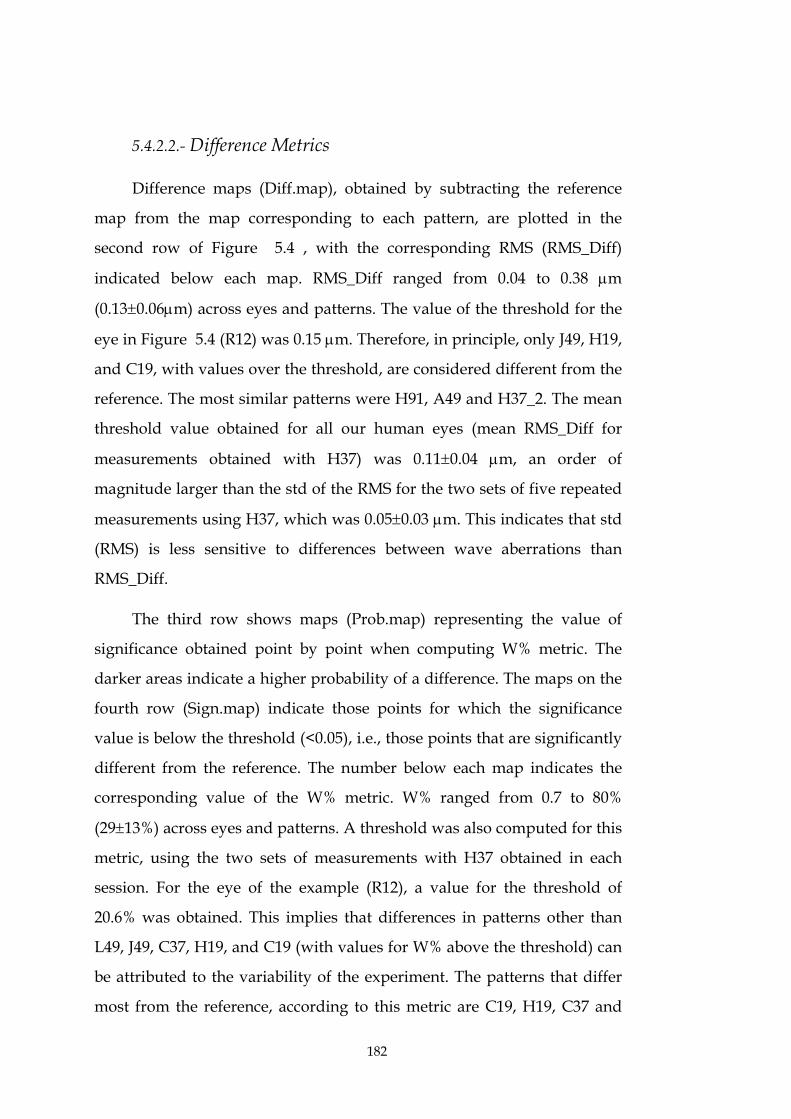
5.4.2.2.- Difference Metrics

Difference maps (Diff.map), obtained by subtracting the reference

map from the map corresponding to each pattern, are plotted in the

second row of Figure 5.4 , with the corresponding RMS (RMS_Diff)

indicated below each map. RMS_Diff ranged from 0.04 to 0.38 μm

(0.13±0.06μm) across eyes and patterns. The value of the threshold for the

eye in Figure 5.4 (R12) was 0.15 μm. Therefore, in principle, only J49, H19,

and C19, with values over the threshold, are considered different from the

reference. The most similar patterns were H91, A49 and H37_2. The mean

threshold value obtained for all our human eyes (mean RMS_Diff for

measurements obtained with H37) was 0.11±0.04 μm, an order of

magnitude larger than the std of the RMS for the two sets of five repeated

measurements using H37, which was 0.05±0.03 μm. This indicates that std

(RMS) is less sensitive to differences between wave aberrations than

RMS_Diff.

The third row shows maps (Prob.map) representing the value of

significance obtained point by point when computing W% metric. The

darker areas indicate a higher probability of a difference. The maps on the

fourth row (Sign.map) indicate those points for which the significance

value is below the threshold (<0.05), i.e., those points that are significantly

different from the reference. The number below each map indicates the

corresponding value of the W% metric. W% ranged from 0.7 to 80%

(29±13%) across eyes and patterns. A threshold was also computed for this

metric, using the two sets of measurements with H37 obtained in each

session. For the eye of the example (R12), a value for the threshold of

20.6% was obtained. This implies that differences in patterns other than

L49, J49, C37, H19, and C19 (with values for W% above the threshold) can

be attributed to the variability of the experiment. The patterns that differ

most from the reference, according to this metric are C19, H19, C37 and

183

J49. Although H37_2, C91 and A49 are the most similar patterns to the

reference, the differences are not significant, according to the threshold.

Figure 5.5 A and B show the results obtained for the metrics

RMS_Diff and W%, respectively, after Ranking across all the human eyes.

The scale for the y axis indicates the value that each pattern was assigned

in the Ranking. This means that the “best” possible score for the ordinate

(y) would be 12 (for a pattern that was the most similar to the reference for

each of the twelve eyes). Similarly, for a pattern being the least similar to

the reference for each of the twelve eyes, the ordinate value would be 120

(12 eyes*10 patterns). In both graphs, patterns are sorted from smallest to

greatest value of the metric, i.e., from most to least similarity with the

reference. The resulting order of the patterns is very similar for both

metrics, showing that the worst results are obtained for the 19-sample

patterns. The best results are obtained for H91, A49, L49 and H37. The H

patterns were found to provide in general better results than C patterns

(for thirty seven and nineteen samples), in the Ranking for both metrics.

Among the forty nine samples patterns, J49 produced the worst results.

184

Figure 5.5. Ranking values for RMS_Diff (A and D) and W% (B and E) corresponding to each sampling pattern across the measured and simulated human eyes, respectively, and. dendrograms from the HCA for the measured (C) and simulated (F) human eyes. Solid green, dashed amber and red dotted lines indicate “good”, “medium” and “bad “ clusters, according to the classification obtained from the metrics. “Dist.” stands for “Distance”.

185

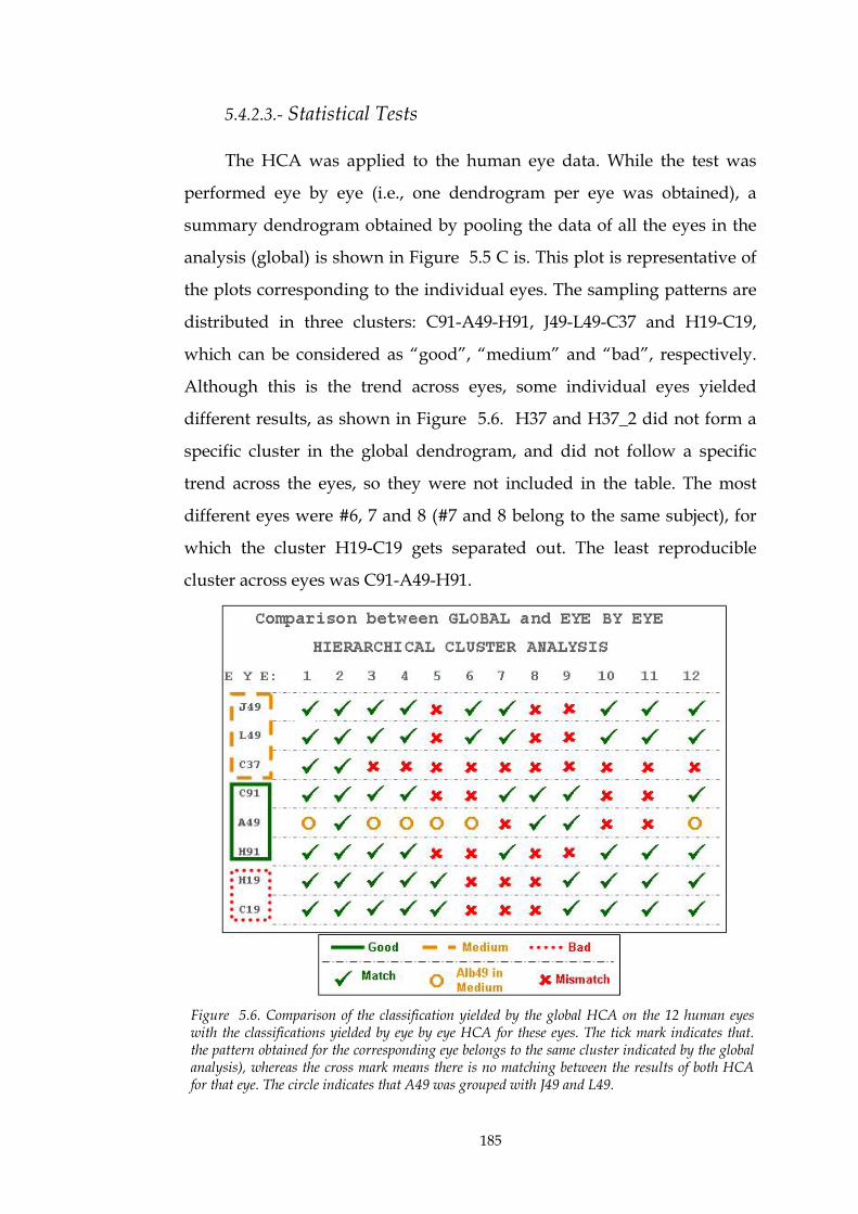
5.4.2.3.- Statistical Tests

The HCA was applied to the human eye data. While the test was

performed eye by eye (i.e., one dendrogram per eye was obtained), a

summary dendrogram obtained by pooling the data of all the eyes in the

analysis (global) is shown in Figure 5.5 C is. This plot is representative of

the plots corresponding to the individual eyes. The sampling patterns are

distributed in three clusters: C91-A49-H91, J49-L49-C37 and H19-C19,

which can be considered as “good”, “medium” and “bad”, respectively.

Although this is the trend across eyes, some individual eyes yielded

different results, as shown in Figure 5.6. H37 and H37_2 did not form a

specific cluster in the global dendrogram, and did not follow a specific

trend across the eyes, so they were not included in the table. The most

different eyes were #6, 7 and 8 (#7 and 8 belong to the same subject), for

which the cluster H19-C19 gets separated out. The least reproducible

cluster across eyes was C91-A49-H91.

Figure 5.6. Comparison of the classification yielded by the global HCA on the 12 human eyes with the classifications yielded by eye by eye HCA for these eyes. The tick mark indicates that. the pattern obtained for the corresponding eye belongs to the same cluster indicated by the global analysis), whereas the cross mark means there is no matching between the results of both HCA for that eye. The circle indicates that A49 was grouped with J49 and L49.

186

The patterns showing more differences according to the t-test were

C19 (4.7%) and H19 (6.4%), and those showing less differences were H37,

H91, C37 and C91 (1.01% each). Differences were found only for the

following coefficients: Z-37 (2.20%), Z-17 (3.30%), Z-15 (4.40%), Z04 (5.50%),

Z02 (12.09%), and Z06 (13.19%).

To summarize, similar results were obtained using both metrics

comparing the shape of the wave aberrations (which depends on our

reference) in consistency with the cluster analysis (which does not depend

on the reference): C91, A49 and H37 were the best patterns and C19, L49

and H37_2 the worst. However, the differences were of the order of the

variability in most cases. When computing the percentage of differing

patterns, those showing most differences were C19 and H19, whereas H37,

H91, C37 and C91 showed the least differences. Regarding Zernike

coefficients, only a few coefficients were significantly different: 37−Z , 1

7−Z ,

15−Z , 0

4Z , 02Z , and 0

6Z .

5.4.3.- NUMERICAL SIMULATIONS

Figure 5.5 D and E show the Ranking plot for RMS_Diff and for W%,

respectively, and Figure 5.5 F shows the dendrogram corresponding to

the global HCA (i.e. including all the eyes) for the simulated human eyes.

The results of the global HCA are presented, similar to the experimental

data, as a summary of the results for each of the twelve simulated eyes.

Similar trends to the measured human eyes are seen, with the main

clusters repeating, although individual pairings changed. As with the

measured human eyes, shown in Figure 5.5 C, H91, C91 and A49 are in

the “good” group, J49 and L49 belong to the “medium” group, and H37,

H19 and C19, although not clearly within any group, appear in borderline

positions. The pattern R177 was included in the “good” group.

Figure 5.7 shows the results obtained for the three simulated

pathological/surgical eyes, for RMS_Diff (A, B and C), for W% (D, E and

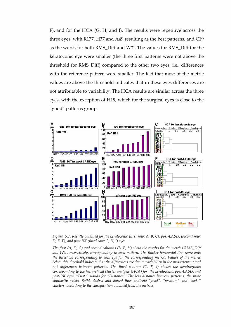
187

F), and for the HCA (G, H, and I). The results were repetitive across the

three eyes, with R177, H37 and A49 resulting as the best patterns, and C19

as the worst, for both RMS_Diff and W%. The values for RMS_Diff for the

keratoconic eye were smaller (the three first patterns were not above the

threshold for RMS_Diff) compared to the other two eyes, i.e., differences

with the reference pattern were smaller. The fact that most of the metric

values are above the threshold indicates that in these eyes differences are

not attributable to variability. The HCA results are similar across the three

eyes, with the exception of H19, which for the surgical eyes is close to the

“good” patterns group.

Figure 5.7. Results obtained for the keratoconic (first row: A, B, C), post-LASIK (second row: D, E, F), and post RK (third row: G, H, I) eyes.

The first (A, D, G) and second columns (B, E, H) show the results for the metrics RMS_Diff and W%, respectively, corresponding to each pattern. The thicker horizontal line represents the threshold corresponding to each eye for the corresponding metric. Values of the metric below this threshold indicate that the differences are due to variability in the measurement and not differences between patterns. The third column (C, F, I) shows the dendrograms corresponding to the hierarchical cluster analysis (HCA) for the keratoconic, post-LASIK and post-RK eyes. “Dist.” stands for “Distance”. The less distance between patterns, the more similarity exists. Solid, dashed and dotted lines indicate “good”, “medium” and “bad “ clusters, according to the classification obtained from the metrics.

188

5.5.- DISCUSSION

5.5.1.- ARTIFICIAL AND HUMAN EYES

Artificial eyes are a good starting point to study experimentally

differences in the sampling patterns for wavefront sensing because they

have fewer sources of variability (only those attributable to the

measurement system, such as thermal noise in the CCD, photon noise,

etc.) than real human eyes (including also variability due to the subject

such as eye movements or microfluctuations of accommodation). The

centroiding noise was estimated by computing the std of the coordinates

of the centroids for each sample across different repetitions for pattern

H37. The mean error averaged between x and y coordinates was 0.09 mrad

for artificial eyes (37 samples and three eyes) and 0.34 mrad for human

eyes (37 samples and twelve eyes). RMS_Diff seems to be a good metric

for artificial eyes, since it provides quantitative differences between the

patterns. However, it would be desirable to rely on an objective

independent reference for the computation of this metric, such as an

interferogram. The differences in the ordering observed with eye A2 (with

no higher terms than SA), where patterns with less samples gave slightly

better results than for the other eyes, supports the idea that the wave

aberrations present in each particular eye affect the optimum pattern, as

would be expected from sampling theory. This finding was fundamental

in previous theoretical work (Diaz-Santana et al., 2005, Soloviev and

Vdovin, 2005), where the statistics of the aberrations to be measured is an

input of the analytical models. The different sorting orders for repeated

measures of the same pattern (H37, H37_2, H37_3, and H37_4) indicate

that the differences of this magnitude are not significant. However, the

sorting of the different patterns is consistent across metrics and statistics

for each eye. To evaluate if sample density affects variability, the std of

189

RMS_Diff across eyes was computed for each pattern, and then the

patterns were sorted in descending order, according to their

corresponding variability. The worst patterns (C37, H19, C19, R21) also

showed a larger variability, indicating that they were less accurate when

sampling the aberrations pattern, in agreement with Diaz-Santana et al.

(2005).

Conclusions based on the artificial eyes have the advantage of

avoiding biological variability, but are restricted because they have very

different aberration structures than human eyes. In our human eyes, the

RMS_Diff metric allowed us to sort the patterns systematically, and the

values of the metric obtained for human and artificial eyes were of the

same order. The W% metric was consistent with RMS_Diff, and more

sensitive. The Ranking procedure was successful at summarizing

information obtained from the metrics, since the metric values are not as

important as sorting the patterns within each eye. However, the main

drawbacks of this procedure are that it does not provide information on

statistical significance (although the results for the same pattern, H37,

obtained for different measurements help to establish significant

differences), and that the conclusions are relative to our reference,

obtained in the same conditions as the assessed patterns, and therefore

these rankings might be dependant on the chosen reference. These

drawbacks are overcome by the HCA which classifies the patterns into

different groups according to the values of the corresponding vectors of

Zernike coefficients and therefore distinguishes between patterns yielding

different results. It also helps to place the results obtained from the metrics

in a more general context. Same as with the artificial eyes, the grouping of

the sampling patterns is consistent across metrics. The spatial distribution

of the samples is important, given that some patterns with the same

number of samples (49) fall into the same group or can even be worse than

patterns with a lower number of samples. Similarly, a “good” sampling

pattern (A49) is grouped with patterns with a larger number of samples.

190

However, for the real eyes, the conclusions are weaker than for artificial

eyes (only differences in patterns with 19 samples are significant),

presumably because biological variability plays a major role, and because

they have a discrete number of modes compared to human eyes, where

the magnitude of the modes keeps decreasing as the orders increase (see

Chapter 1, section 1.2.4.1). Overall, the undersampling patterns C19 and

H19 were consistently amongst the most variable patterns, and this was

confirmed by the ANOVA for Zernike coefficients. Long term drift was

not problematic in these eyes, since final H37 measurements were not

more variable than the standard measurements.

Measurement errors in human eyes prevented from finding

statistically significant differences between most sampling patterns.

However, stds of repeated measurements of this study were less or equal

to other studies. The mean variability across patterns and eyes for our

human eyes was 0.02 μm (average std across runs of the Zernike

coefficient, excluding tilts and piston) for Zernike coefficients. This value

is smaller than those obtained by Moreno-Barriuso et al. (2001a) on one

subject measured with a previous version of the LRT system (0.06 μm),

with a HS sensor (0.07 μm) and a Spatially Resolved Refractometer (0.08

μm), and than those obtained by Marcos et al. (2002b), using the same LRT

device (0.07 μm for 60 eyes), and a different HS sensor (0.04 μm for 11

eyes). A similar value (0.02 μm) is obtained when computing the average

of the std of the Zernike coefficients (excluding piston and tilts)

corresponding to the eye reported by Davies et al. (2003) using HS. The

negligible contribution of random pupil shifts during the measurements

on the wave aberration measurement and sampling pattern analysis was

further studied by examining the effective entry pupils obtained from

passive eye-tracking analysis. The most variable set of series (according to

std of RMS, and std of Zernike coefficients across series), which

corresponded to Eyes #1 (H19) and 2 (H37_2), respectively, was selected.

Absolute random pupil shifts across the measurements were less than 0.17

191

mm for coordinate x and 0.11 mm for coordinate y. The mean shift of the

pupil from the optical axis (i.e. centration errors, to which both sequential

and non-sequential aberrometers can be equally subject) was in general

larger than random variations. The estimates of the wave aberrations

obtained using the nominal entry pupils were compated to those obtained

using the actual pupil coordinates (obtained from passive eye tracking

routines). When pupil shifts were accounted for by using actual

coordinates, measurement variability remained practically constant both

in terms of RMS std (changing from 0.09 when nominal coordinates were

used to 0.07 μm when actual coordinates were used and from 0.14 to 0.13

μm for eyes #1 and 2 respectively), and in terms of average Zernike

coefficients std (changing from 0.06 when nominal coordinates were used

to 0.05 μm when actual coordinates were used and from 0.03 to 0.03 μm,

for eyes #1 and 2, respectively). On the other hand, the differences

between average RMS using nominal or actual entry locations (0.51 μm vs

0.49 μm for eye #1 and 0.61 μm vs 0.59 μm for eye #2) are negligible. Also,

RMS_Diff values (using the wave aberrations with nominal entry locations

as a reference, and wave aberrations with the actual entry locations as a

test), 0.02±0.01 μm for eye #1 (mean±std across repeated measurements for

the same pattern), and 0.04±0.02 μm for eye #2, are below the threshold for

these eyes.

5.5.2.- NUMERICAL SIMULATIONS

It has been shown with artificial eyes that sampling patterns with a

small number of samples (19) are good at sampling aberration patterns

with no higher order terms (eye A2), as expected from sampling theory.

When analyzing our ranking results on normal human eyes, remarkable

differences were found only in the patterns with a small number of

samples. This is due to the presence of higher order aberrations and larger

measurement variability in these eyes.

192

Due to the lack of a “gold standard” measurement, there are some

issues that have not been addressed in the experimental part of this work,

such as: 1) Does the magnitude of some particular aberrations determine

a specific pattern as more suitable than others to sample that particular

eye?; 2) Will eyes with aberration terms above the number of samples be

properly characterised using the different patterns?; 3) Will measurements

in eyes with aberration terms of larger magnitude than normal eyes yield

different results?. From the results shown in section 5.3.4.4.- it can be

concluded that the simulations provide a good estimate of the

performance of the repeated measurements using different sampling

schemes in real normal human eyes. Therefore, computer simulations

were used as a tool to address these issues.

From the results corresponding to the pathological/surgical eyes, it

should be noted that: 1) The pattern H37 is consistently classified as the

best pattern apparently because this is the pattern used to perform the

original measurement of aberrations from which the wave aberration was

computed for the simulations; 2) The variability values used in the

simulations were obtained from normal eyes, and they may be smaller

than those corresponding to pathological/surgical eyes; 3) The pattern

H19 was close to the “good” patterns group for the surgical eyes only,

what may be due to the predominance of SA, characteristic of these eyes..

Although the values of the metrics are larger for these

pathological/surgical eyes, the conclusions obtained from our real eyes

seem applicable to eyes with greater amounts of aberrations: even though

patterns with more samples tend to give better results, the spatial

distribution of the samples is important. While a large number of samples

helps (R177), the correct pattern at lower sampling was more efficient

(A49, H91) for eyes dominated by some specific aberrations.

It should be pointed out that the conclusions related to pathological

eyes displayed in this section are obtained from simulations, and should

193

be regarded as a preliminary approximation to the study of sampling

pattern in pathological eyes, which should include experimental data.

5.5.3.- COMPARISON TO PREVIOUS LITERATURE

Díaz-Santana et al.’s analytical model (Diaz-Santana et al., 2005),

previously described in the introduction of this chapter, allowed them to

test theoretically different sampling patterns using as a metric the RMS

introduced in wave aberration measurements by the different geometries.

This model uses as an input the second order statistics of the population

and hence it is bound to include the interactions reported by McLellan et

al. (2006), as long as the population sample and number of Zernike terms

are large enough to reflect all possible interactions. This fact also implies

that the conclusions of their model are strongly dependent on the

characteristics of the population. As an example, they applied their model

to a population of 93 healthy non-surgical eyes, with aberration terms up

to the 4th order, to compare square, hexagonal and polar geometries. They

found that, for their population, the sampling density did not influence

much RMS error for hexagonal and square grids, whereas lower sampling

densities produced a smaller error for polar grids. When comparing grids

with different geometries and similar densities they found, in agreement

with our results, that the polar geometry was best (in terms of smaller

error), followed by the hexagonal grid. Differences in performance

between patterns decreased as density increased.

Soloviev et al.’s analytic model (Soloviev and Vdovin, 2005) of

Kolmogorov’s statistics, indicates that random sampling produces better

results than regularly spaced ones. They also reported that aliasing error

increases dramatically for regular samplings for fits reconstructing more

modes, whereas the associated error of the HS sensor was smaller for

irregular masks (with 61 subapertures of 1/11 of the pupil diameter of

size), probably because an irregular geometry helps to avoid cross-

coupling. Our experimental study supports their conclusion that simply

194

increasing the number of samples does not necessarily decrease the error

of measurement, and that sampling geometry is important.

In the current study, the Zernike modal fitting was used to represent

the wave aberration because it is the standard for describing ocular

aberrations. Smolek and Klyce (Smolek and Klyce, 2003) questioned the

suitability of Zernike modal fitting to represent aberrations in eyes with a

high amount of aberrations (keratoconus and post-keratoplasty eyes),

reporting that the fit error had influence in the subject’s best corrected

spectacle visual acuity. Marsack et al. (2006) revisited this question

recently concluding that only in cases of severe keratoconus (with a

maximum corneal curvature over 60 D), Zernike modal fitting failed to

represent visually important aberrations. In the current study this

question was not addressed, but our conditions were rather restricted to

those more commonly encountered, and for which Zernike modal fitting is

expected to be adequate.

5.5.4.- CONCLUSIONS

From this study we can conclude:

1) Comparison of optical aberrations of healthy non surgical human

and artificial eyes measured using different sampling patterns allowed us

to examine the adequacy of two spatial metrics, the RMS of difference

maps and the wave aberration difference (W%) to compare estimates of

aberrations across sampling schemes.

2) For artificial eyes, there is an interaction of the aberrations present

and the ability of a given spatial sampling pattern to reliably measure the

aberrations. Simply increasing the number of samples was not always as

effective as choosing a better sampling pattern.

3) Moderate density sampling patterns based on the zeroes of

Albrecht’s cubature (A49) or hexagonal sampling performed relatively

well.

195

4) For normal human eyes individual variability in local slope

measurements was larger than the sampling effects, except, as expected,

for undersampling patterns (H19 and C19). However, in these eyes it has

also been found that the spatial distribution of the sampling can be more

important than the number of samples: A49 and H37 were a good

compromise between accuracy and density.

5) The numerical simulations are a useful tool to a priori assess the

performance of different sampling patterns when measuring specific

aberration patterns, since in general, the results are similar to those found

for our measured normal human eyes.

This study should be taken as a first experimental approach to the

problem of finding optimal patterns. Future studies on a larger number of

eyes and with very different aberration patterns should be carried out in

order to find the different patterns more suitable for different groups of

population (young eyes or myopic eyes for example) or specific conditions

(keratoconic or postsurgical eyes). However, finding a generic pattern that

performs relatively well for general population is also necessary for

screening and quick characterisation of the aberration pattern. Also, a

reference independent of any particular sampling pattern is desirable in

order to have a gold standard to compare to, rather than assume the

“goodness” of some patterns.

Finally, the implementation of some of the patterns presented in this

study in a HS, for example, would not be straight forward. Even if the

manufacturers could produce lenslets distributed according to Jacobi,

Legendre or Albrecht patterns, there are some issues such as the loss of

resolution in those locations where the lenslets are too close (leakage of

light from a lenslet into the pixels corresponding to the neighbour lenslet)

that should be solved.

196