CHAPTER 4 WAVELET ANALYSIS OF …shodhganga.inflibnet.ac.in/bitstream/10603/16353/9/09_chapter4.pdf · CHAPTER 4 WAVELET ANALYSIS OF ELECTROGASTROGRAM SIGNALS 4.1 INTRODUCTION Biosignals

79

CHAPTER 4

WAVELET ANALYSIS OF ELECTROGASTROGRAM

SIGNALS

4.1 INTRODUCTION

Biosignals are used in the biomedical field mostly for the

investigation of the subject’s biological system by extracting its features.

Electrogastrogram [EGG], a non-stationary signal acquired cutaneously is a

non-invasive method of detecting the disorders of a digestive system. The

physician may have this as a preliminary investigation before going for the

Endoscopic procedure. In this chapter, investigation is performed to identify

the digestive system disorders present in EGG signals using Wavelet

Transform. The signal is analyzed using Continuous Wavelet Transform

(CWT) and Discrete Wavelet Transform (DWT). In CWT, the subjects are

classified according to number of peaks obtained. In DWT, the EGG signal is

first decomposed and then it is reconstructed to find the threshold value to

classify the different digestive disorder subjects. The EGG signals are

subjected to 3 levels of decomposition using Daubechies mother wavelet.

Wavelet Transform (WT) was introduced at the beginning of the

1980s by Morlet et al Since then, various types of wavelet transforms have

been developed, and many other applications have been found (Burrus et al

1998). The continuous-time wavelet transform, also called the Integral

Wavelet Transform (IWT), finds most of its applications in data analysis,

where it yields an affine invariant time-frequency representation. DWT has

80

excellent signal compaction properties for many classes of real-world signals

while being computationally very efficient. Therefore, it has been applied to

almost all technical fields including image compression, denoising, numerical

integration, and pattern recognition.

WT has similarities with the Short-Time Fourier Transform, but it

also possesses a time-localization property that generally renders it superior

for analyzing non-stationary signals such as EGG. WT also decompose a

signal into a set of “frequency bands” (referred to as scales) by projecting the

signal onto an element of a set of basic functions. Although the scales do not

live in the frequency domain, projection of the signal onto different scales is

equivalent to bandpass filtering with a bank of constant-Q filters. The basic

functions are called wavelets. Wavelets in a basis are all similar to each other,

varying only by dilation and translation. In wavelet analysis, one looks at the

signals at different scales or resolution. A rough approximation of the signal

might look stationary; while at a detailed level when using small window,

discontinuities become evident.

4.2 LITERATURE REVIEW

Akhilesh Bijalwan et al (2012) deals with the threshold estimation

method for image denoising in the wavelet transform domain. The technique

is based upon the discrete wavelet transform analysis where the algorithm of

wavelet threshold is used to calculate the value of threshold. Experimental

results on several test images are compared with denoising techniques based

on Peak Signal to Noise ratio (PSNR), Root Mean Square Error (RMSE) and

Correlation of Coefficient (CoC). Rui Rodrigues and Paula Couto (2012)

proposed an ECG denoising method based on a feed forward neural network

with three hidden layers. Particularly useful for very noisy signals, this

approach uses the available ECG channels to reconstruct a noisy channel by

adding noise to an existing signal and measure the RMSE of the denoised

81

signal relative to the original signal. Shantanu Godbole (2012) has shown

various ways in which the notion of similarity amongst subsets of classes

from the confusion matrix can be exploited. First, the author has provided a

mechanism of generating more meaningful intermediate levels of hierarchies

in large at sets of classes. Secondly, the author has demonstrated on how large

multi-class classification tasks can be scaled up with the number of classes.

Barroso-Alvarado et al (2011) reported db4 wavelet analysis on

EGG database. Classical parameters namely mean, standard deviation,

dominant frequency and dominant power are analyzed. Suman et al (2011)

proposed the adaptive noise canceller that has been optimized with Modified

Memetic Algorithm (MMA) to remove power line interference in the ECG

signals. The performance of these algorithms has been analyzed on the basis

of parameters viz., improvement in signal to noise ratio, normalized

correlation coefficient (NCC) and root mean square error (RMSE).

Nagendra.H (2011) has provided an overview of some wavelet techniques

namely CWT, DWT, Stationary WT, Fractional WT. Performance is

evaluated using RMSE. Powers, D.M.W (2011) used evaluation measures

including Recall, Precision, F-Measure and Accuracy for concepts of

Informedness, Markedness, Correlation and Significance, as well as analyzed

the intuitive relationships of Recall and Precision, and outlined the extension

from the dichotomous case to the general multi-class case.

Curilem et al (2010) compared ANN and SVM for EGG analysis

and showed SVM classifier is faster, requires less memory than ANN. Wei

Ding et al (2010) utilized Electrogastrography to detect slow wave of gastric

digest motility after test meal and the authors used multiresolution method

with the Daubechies wavelet function to decompose EGG signal. Abdel-

Reman et al (2010) used the high pass filtering for noisy signal before

82

reconstruction by inverse discrete wavelet transform (IDWT). This algorithm

is very robust for noise removal in Electrocardiogram (ECG).

Chacon et al (2009) analyzed neural network structures to classify

the wavelet coefficient for healthy and dyspepsia patients. The classifier

achieved 78.6 % sensitivity and 92.9 % specificity and Classification

Accuracy of 82.1%. TanYun-fu et al (2009) used Daubechies and Symlet

wavelets for the removal of various kinds of noises present in the ECG signal

and reconstructed ECG signal with minimum distortion at a faster rate.

Saritha et al (2008) identified different types of abnormalities in ECG using

daubechies wavelets in MATLAB environment.

Wei Zhang et al (2008) used the multiresolution concept along with

adaptive filters to detect effectively, the weak ECG signal in strong noisy

environment. Cheng Peng et al (2007) applied independent component

analysis with references to separate the gastric signal from noises. Mahumut

Tokmakei (2007) analyzed EGG using discrete wavelet transform and

statistical methods to detect gastric dysrhytmia. Kania et al (2007) studied the

importance of the proper selection of mother wavelet with appropriate number

of decomposition levels for reducing the noise in ECG signal. The authors

claim that they obtained good quality signal for the wavelet db1 at first and

fourth level of decomposition and at fourth level of decomposition for sym3.

Dirgenali et al (2006) compared wavelet method and short-time

Fourier transform method to find abnormalities of EGG signals and showed

that WT sonograms can be used to classify patients successfully. Kara et al

(2006) developed a method for EGG classification based on DWT and ANN.

This method achieved 98.5% sensitivity and 94.5% specificity. Tchervensky

et al (2006) utilized wavelet-based decomposition technique to process

multichannel EGG signals. The authors considered this to be an effective

method for enhancing the clinical utility of EGG. Choukari et al (2006) used

83

second level decomposition for detecting QRS complex and fourth and fifth

level of decomposition for detecting P and T waves in ECG. Brij Singh and

Arvind Tiwari (2006) presented a selection procedure of mother wavelet

basis functions applied for denoising of the ECG signal in wavelet domain

while retaining the signal peaks close to their full amplitude. The obtained

wavelet based denoised ECG signals retain the necessary diagnostics

information contained in the original ECG signal. The experimental results

have revealed suitability of Daubechies mother wavelet of order 8 to be the

most appropriate wavelet basis function for the denoising application (Parmod

and Devanjali 2010).

Kara et al (2005) performed wavelet packet analysis of EGG

signals and estimated gastric rhythm differences of normal and diabetic

subjects. Liang (2005) used a combined method of stages combined method

with independent component analysis and adaptive signal enhancement for

extraction of gastric slow waves from EGG or to detect propagation of gastric

slow waves from multichannel EGG. Amit C. Patel and Mia K. Markey

(2005) empirically compared the methods that have been proposed to evaluate

the performance of N-class classifiers (N>2). Morteza Moazami-Goudarzi

(2005) assessed the functionality of the different multiwavelets in

compressing ECG signals, in addition to known factors such as Compression

Ratio (CR), Percent Root Difference (PRD), Distortion (D), and Root Mean

Square Error (RMSE) in compression literature.

De Sobral Cintra (2004) proposed that matching a wavelet to a

class of signals can be of interest in feature detection and classification based

on wavelet representation. The authors provided a quantitative approach and

wavelets generated from the optimal parameterization values were similar to

the standard db3 wavelet and were used to the problem of matching a wavelet

to EGG signals. Hualou Liang and Zhiyue Lin (2002) provided a description

84

of two multiresolution methods for electrogastric signal processing, namely,

wavelet transform and empirical mode decomposition in their paper. Zhenghu

et al (2000) developed a new method for processing EGG signals based on

wavelet transform which has a very good application perspective because it is

found to be simple and a convenient way to provide precise charts and

recognition about frequency characteristic to a refinement. Han-Chang Wu

(1998) considered EGG to be more important due to its non-invasive

measurement and the authors have developed a new method based on discrete

wavelet transform (DWT) to analyze the power distribution of the EGG

signals. Jie Liang (1997) applied Nonorthogonal Multiresolution Wavelet

Analysis (NOMRWA) on EGG noise detection and denoising.

4.3 CONTINUOUS WAVELET TRANSFORM

Continuous Wavelet Transform (CWT) was developed as an

alternative approach to the FT to reduce the difficulty in extracting

information from the signals. The term wavelet means a small wave. The

smallness refers to the condition that this function is of finite length. The

wave refers to the condition that this function is oscillatory. For getting the

CWT of a signal, the signal is multiplied with a function (wavelet), and the

transform is computed separately for different segments of the time domain

signal.

Continuous Wavelet Transform is defined by Equation (4.1)

dts

ttxs

ssCWT xx

*1,, (4.1)

where,

τ : translation parameter

85

s : scaling parameter

(t) : mother wavelet

tx : input signal

The transformed signal is a function of two variables ‘τ’ and ‘s’,

the translation and scale parameters, respectively. Thus, the wavelet transform

is computed as the inner product of x (t) and translated and scaled versions of

a single function (t), which is called wavelet. (t) is the transforming

function, and it is called the mother wavelet. The term mother implies that the

functions with different region of support that are used in the transformation

process are derived from one main function, or the mother wavelet. The

mother wavelet is a prototype for generating the other window functions. The

term translation refers to the location of the window, as the window is shifted

through the signal.

In wavelet analysis, high scales correspond to a non-detailed view

of the signal, and low scales correspond to a detailed view. Similarly, in terms

of frequency, low frequencies (high scales) correspond to a global

information of a signal (that usually spans the entire signal), whereas high

frequencies (low scales) correspond to a detailed information of a hidden

pattern in the signal (that usually lasts a relatively short time).

In most of the bio-signals, low scales (high frequencies) do not last

for the entire duration of the signal, but they usually appear from time to time

as short bursts, or spikes. High scales (low frequencies) usually last for the

entire duration of the signal. Scaling, as a mathematical operation, either

dilates or compresses a signal. Larger scales correspond to dilated (or

stretched out) signals and small scales correspond to compressed signals.

86

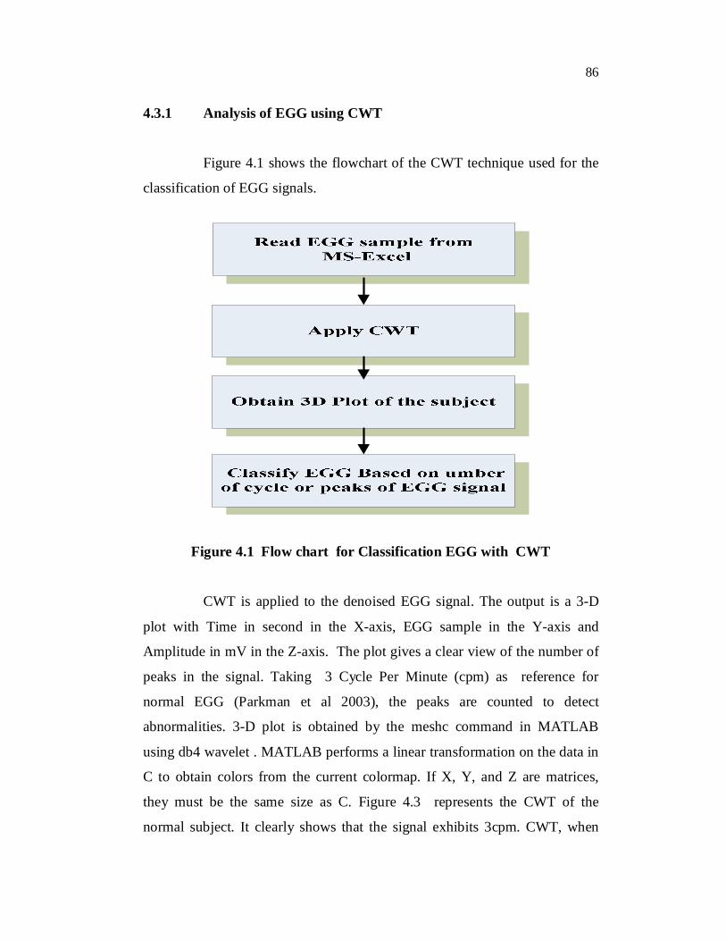
4.3.1 Analysis of EGG using CWT

Figure 4.1 shows the flowchart of the CWT technique used for the

classification of EGG signals.

Figure 4.1 Flow chart for Classification EGG with CWT

CWT is applied to the denoised EGG signal. The output is a 3-D

plot with Time in second in the X-axis, EGG sample in the Y-axis and

Amplitude in mV in the Z-axis. The plot gives a clear view of the number of

peaks in the signal. Taking 3 Cycle Per Minute (cpm) as reference for

normal EGG (Parkman et al 2003), the peaks are counted to detect

abnormalities. 3-D plot is obtained by the meshc command in MATLAB

using db4 wavelet . MATLAB performs a linear transformation on the data in

C to obtain colors from the current colormap. If X, Y, and Z are matrices,

they must be the same size as C. Figure 4.3 represents the CWT of the

normal subject. It clearly shows that the signal exhibits 3cpm. CWT, when

87

applied to raw EGG data and showed unclear peaks for normal EGG as in

Figure 4.2. Due to the presence of unclear peaks, the Classification Accuracy

was found to be 61.71% for normal EGG. Hence all the signal were denoised

and then analysed.

Figure 4.2 CWT of raw EGG for Normal Subject

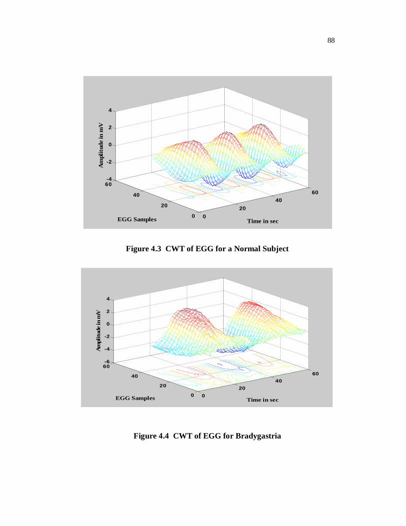
The reference signal obtained from the physician for normal and

dysarrthymic EGG signals when subjected to CWT analysis showed distinct

peaks for each type of EGG as depicted in Figure.4.3 for normal subjects,

Figure.4.4 for bradygastria subjects, Figure.4.5 for dyspepsia subjects,

Figure.4.6 for nausea subjects , Figure.4.7 for ulcer subjects , Figure.4.8 for

tachygastria subjects and Figure.4.9 for vomiting subjects. The cpm

determined by the the 3-D plot for various disorders is tabulated in Table 4.1

and this is used for the classification of disorders.

010

2030

4050

6070

010

2030

4050-3

-2

-1

0

1

2

Time in sec EGG Samples

Am

plitu

de in

mV

88

Figure 4.3 CWT of EGG for a Normal Subject

Figure 4.4 CWT of EGG for Bradygastria

020

4060

0

20

40

60-4

-2

0

2

4

Time in secEGG Samples

Am

plitu

de in

mV

020

4060

0

20

40

60-6

-4

-2

0

2

4


Am

plitu

de in

mV

89

Figure 4.5 CWT of EGG for Dyspepsia

Figure 4.6 CWT of EGG for Nausea

020

4060

0

20

40

60-4

-2

0

2

4


Am

plitu

de in

mV

020

4060

0

20

40

60-3

-2

-1

0

1

2

3


Am

plitu

de in

mV

90

Figure 4.7 CWT of EGG for Tachygastria

Figure 4.8 CWT of EGG for Ulcer

020

4060

0

20

40

60-2

-1

0

1

2


Am

plitu

de in

mV

020

4060

0

20

40

60-3

-2

-1

0

1

2


Am

plitu

de in

mV

91

Figure 4.9 CWT of EGG for Vomiting Condition

Table 4.1 EGG Classification using CWT

Sl.No. EGG Number of peaks ( cpm)

1. Normal 3 2. Bradygastria 1.5 3. Dyspepsia 4 4. Nausea 3.5 5. Tachygastria 8 6. Ulcer 7 7. Vomiting 6

Denoised EGG signal is obtained using filters as given in chapter 2

and these signals are considered for further analysis.

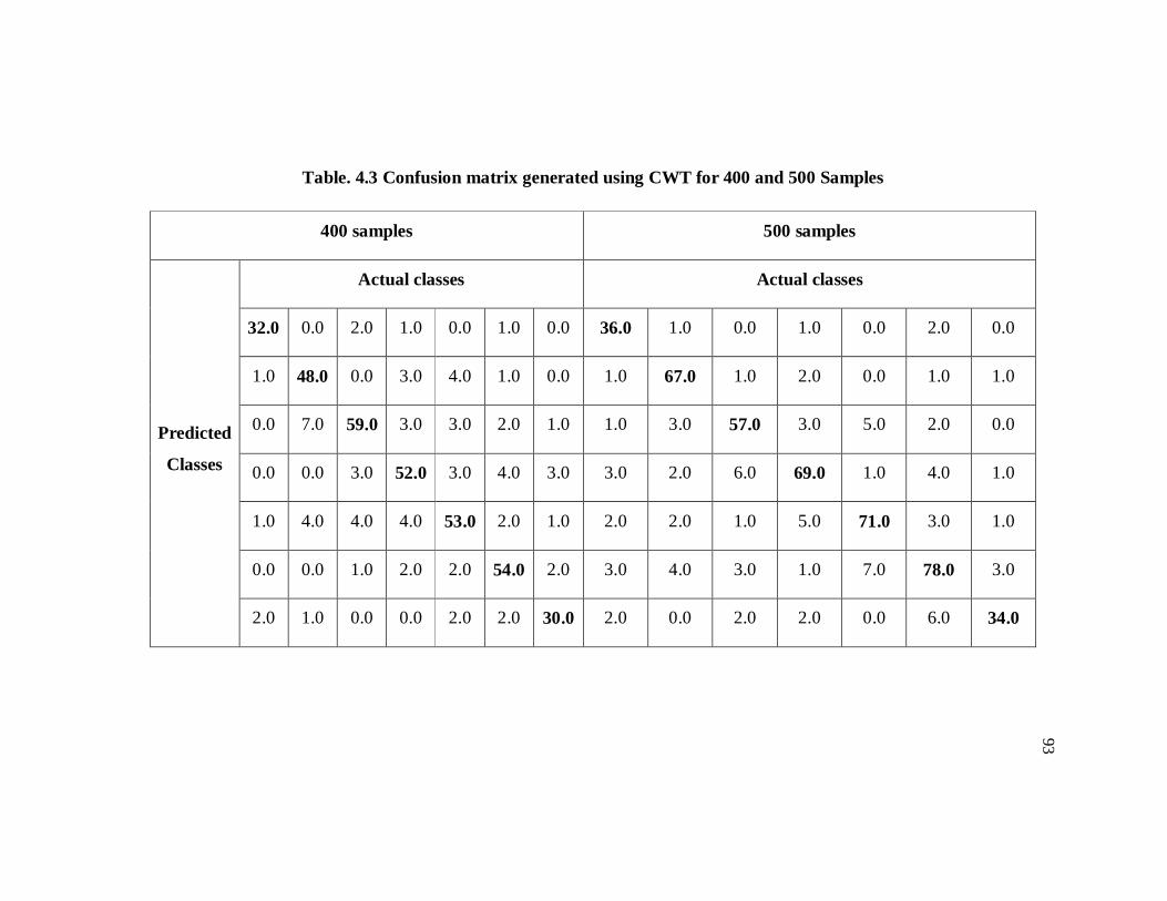
4.3.2 Confusion Matrix for CWT

Confusion matrix is formed for the signals acquired in the

laboratory setup with different composition as in Table 3.5 are tabulated in

Table 4.2 and Table 4.3 for different sample sets.

010

2030

4050

60

0

20

40

60-4

-2

0

2

4


Am

plit

ude

in m

V

92

Table. 4.2 Confusion matrix generated using CWT for 200 and 300 Samples

200 samples 300 samples

Predicted

Classes

Actual classes Actual classes

15.0 0.0 0.0 2.0 0.0 2.0 0.0 14.0 2.0 0.0 2.0 0.0 1.0 0.0

1.0 27.0 3.0 1.0 0.0 1.0 1.0 1.0 41.0 1.0 2.0 1.0 2.0 2.0

0.0 0.0 18.0 1.0 0.0 2.0 0.0 1.0 4.0 46.0 1.0 2.0 1.0 2.0

1.0 0.0 3.0 30.0 3.0 2.0 0.0 0.0 3.0 2.0 35.0 0.0 1.0 0.0

0.0 0.0 2.0 3.0 25.0 1.0 0.0 0.0 1.0 4.0 4.0 45.0 0.0 1.0

0.0 3.0 1.0 0.0 2.0 28.0 2.0 0.0 1.0 2.0 1.0 4.0 41.0 0.0

0.0 2.0 0.0 0.0 0.0 1.0 17.0 0.0 1.0 1.0 0.0 0.0 5.0 21.0

93

Table. 4.3 Confusion matrix generated using CWT for 400 and 500 Samples


Predicted

Classes


32.0 0.0 2.0 1.0 0.0 1.0 0.0 36.0 1.0 0.0 1.0 0.0 2.0 0.0

1.0 48.0 0.0 3.0 4.0 1.0 0.0 1.0 67.0 1.0 2.0 0.0 1.0 1.0

0.0 7.0 59.0 3.0 3.0 2.0 1.0 1.0 3.0 57.0 3.0 5.0 2.0 0.0

0.0 0.0 3.0 52.0 3.0 4.0 3.0 3.0 2.0 6.0 69.0 1.0 4.0 1.0

1.0 4.0 4.0 4.0 53.0 2.0 1.0 2.0 2.0 1.0 5.0 71.0 3.0 1.0

0.0 0.0 1.0 2.0 2.0 54.0 2.0 3.0 4.0 3.0 1.0 7.0 78.0 3.0

2.0 1.0 0.0 0.0 2.0 2.0 30.0 2.0 0.0 2.0 2.0 0.0 6.0 34.0

94

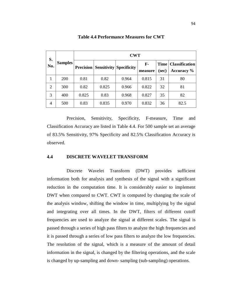
Table 4.4 Performance Measures for CWT

S. No.

Samples

CWT

Precision Sensitivity Specificity F-

measure Time (sec)

Classification Accuracy %

1 200 0.81 0.82 0.964 0.815 31 80

2 300 0.82 0.825 0.966 0.822 32 81

3 400 0.825 0.83 0.968 0.827 35 82

4 500 0.83 0.835 0.970 0.832 36 82.5

Precision, Sensitivity, Specificity, F-measure, Time and

Classification Accuracy are listed in Table 4.4. For 500 sample set an average

of 83.5% Sensitivity, 97% Specificity and 82.5% Classification Accuracy is

observed.

4.4 DISCRETE WAVELET TRANSFORM

Discrete Wavelet Transform (DWT) provides sufficient

information both for analysis and synthesis of the signal with a significant

reduction in the computation time. It is considerably easier to implement

DWT when compared to CWT. CWT is computed by changing the scale of

the analysis window, shifting the window in time, multiplying by the signal

and integrating over all times. In the DWT, filters of different cutoff

frequencies are used to analyze the signal at different scales. The signal is

passed through a series of high pass filters to analyze the high frequencies and

it is passed through a series of low pass filters to analyze the low frequencies.

The resolution of the signal, which is a measure of the amount of detail

information in the signal, is changed by the filtering operations, and the scale

is changed by up-sampling and down- sampling (sub-sampling) operations.

95

Discrete Wavelet Transform analyses the signal at different

frequency bands with different resolutions by decomposing the signal into

coarse approximation and detail information. DWT employs two sets of

functions, called scaling functions and wavelet functions, which are

associated with low pass and high pass filters, respectively (West et al 2006).

The decomposition of the signal into different frequency bands is simply

obtained by successive high pass and low pass filtering of the time domain

signal. The original signal x[n] is first passed through a half band high pass

filter g[n] and a low pass filter h[n]. After filtering, half of the samples can be

eliminated. The signal is then sub sampled by 2, simply by discarding every

other sample. This constitutes one level of decomposition and is mathematically expressed as in Equations (4.2) and (4.3).

nk2gnxky

nhigh (4.2)

nk2hnxkyn

low (4.3)

kyhigh and kylow are the outputs of the high pass and low pass

filters, respectively, after sub-sampling by 2. This decomposition halves the

time resolution since only half the numbers of samples now characterize the

entire signal. But this operation doubles the frequency resolution, since the

frequency band of the signal now spans only half the previous frequency

band, effectively reducing the uncertainty in the frequency by half. This

procedure, also known as the sub-band coding, is repeated for further decomposition.

Multiresolution wavelet description provides for the analysis of the

signal into low pass components at each level of resolution called coarse

signals through C operators (Mallat 1989). At the same time, the detail

component through the D operator provides information regarding bandpass

96

components. With each decreasing resolution level, different signal approximations are made to capture unique signal features.

The flow chart for multiresolution algorithm showing how coarse

and detail component of resolution level j are generated from higher

resolution level 1j is shown in Figure 4.10.

1 jj

fDdj2

fC dj 12

fC dj2

1 jJ

Figure 4.10 Flowchart of Multiresolution Algorithm

Step 1 : Start with N samples of EGG signal x (t) at resolution level j=0.

Step 2 : Convolve the signal with the scaling function φ (t) to find C1f

with j=0.

Step 3 : Find the coarse signal at successive resolution levels, J,.......3,2,1j

Step 4 : Find the detail signal at successive resolution levels,

J,.......3,2,1j : Keep other sample of the output.

Step 5 : Decrease j and repeat steps 3 through 5 until j=-J, where j is

the smallest scaling index.

97

~0f

~

2f

2~0 f

2~

4f

4~

8f

4~0 f

8~0 f

Figure 4.11 Sub-band Decomposition

At every level, the filtering and sub-sampling results in half the

number of samples (and hence half the time resolution) and half the frequency

band spanned (and hence doubles the frequency resolution). Figure 4.11

illustrates this procedure, where x[n] is the original signal to be decomposed,

h[n] and g[n] is high pass and low pass filters respectively. The bandwidth of

the signal at every level is marked as f.

With respect to the Figure 4.11, a signal (S) is segregated into an

approximation (A) and a detail (D) for three level of decomposition and is

given by Equation (4.4).

98

3D2D1D3A2D1D2A1D1AS (4.4)

The approximations are the high-scale, low-frequency components

of the signal. The details are the low-scale, high-frequency components. The

approximation is then itself split into a second-level approximation and detail,

and the process is repeated. For n-level decomposition, there are n+1possible

ways to decompose or encode the signal.

This procedure offers a good time resolution at high frequencies

and good frequency resolution at low frequencies. The frequency bands that

are not very prominent in the original signal have very low amplitudes, and

that part of the DWT signal is discarded without any major loss of

information, allowing data reduction.

4.4.1 Analysis of EGG using DWT

DWT analyzes the EGG signal at different frequency bands with

different resolutions by decomposing the signal into a coarse approximation

and detail information. DWT employs two sets of functions called scaling

functions and wavelet functions, which are associated with low-pass and

high-pass filters, respectively. The decomposition of the signal into the

different frequency bands is simply obtained by successive high-pass and

low-pass filtering of the time domain signal. Figure 4.12 depicts the

classification process with DWT.

Selection of wavelet and number of levels

In DWT signal analysis, the selection of suitable wavelet and the

number of levels of decomposition is very important. A unique way is to have

visual inspection of data, if the data are kind of discontinuous, Haar or other

sharp wavelet functions are adopted otherwise a smoother wavelet can be

99

employed as reported by Subasi (2004). The tests are performed with five

different types of wavelets namely db1, db4, db10, coif5 and sym8 and the

Mean Square Error (MSE) of different levels is tabulated as shown in Table

4.5. From table it is observed that the wavelet function ‘db4’ provides the

reduced MSE values for the different levels.

Figure 4.12 Flow chart for Classification EGG with DWT

Specifically at level 3, db4 has the lowest MSE value compared to

coiflet and symlet. So the wavelet function ‘db4’ is used to decompose the

EGG signal upto level 3.

100

Table 4.5 Selection of Wavelet for DWT

Wavelet MSE

Level 1 Level 2 Level 3 Level 4 Level 5 db1 0.0116 0.0120 0.0136 0.0156 0.0201 db4 0.0113 0.0110 0.0107 0.0117 0.0116

db10 0.0201 0.0243 0.0276 0.0311 0.0309 coif5 0.0152 0.0147 0.0132 0.0142 0.0167 sym8 0.0118 0.0116 0.0117 0.0122 0.0120

The number of levels of decomposition is chosen based on the

dominant frequency components of the signal. The levels are chosen such that

those parts of the signal that correlate well with the frequencies required for

classification of the signal are retained in the wavelet coefficients. In EGG

signals the high level decomposition degrades the value of the signal i.e. for

level above 3 there is no information about the signal so the number of levels

is chosen to be 3. Thus the signal is decomposed into the details D1–D3 and

one final approximation, A3.

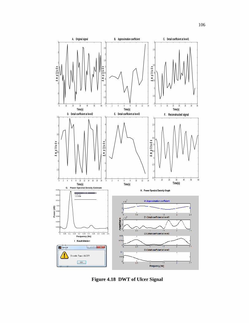
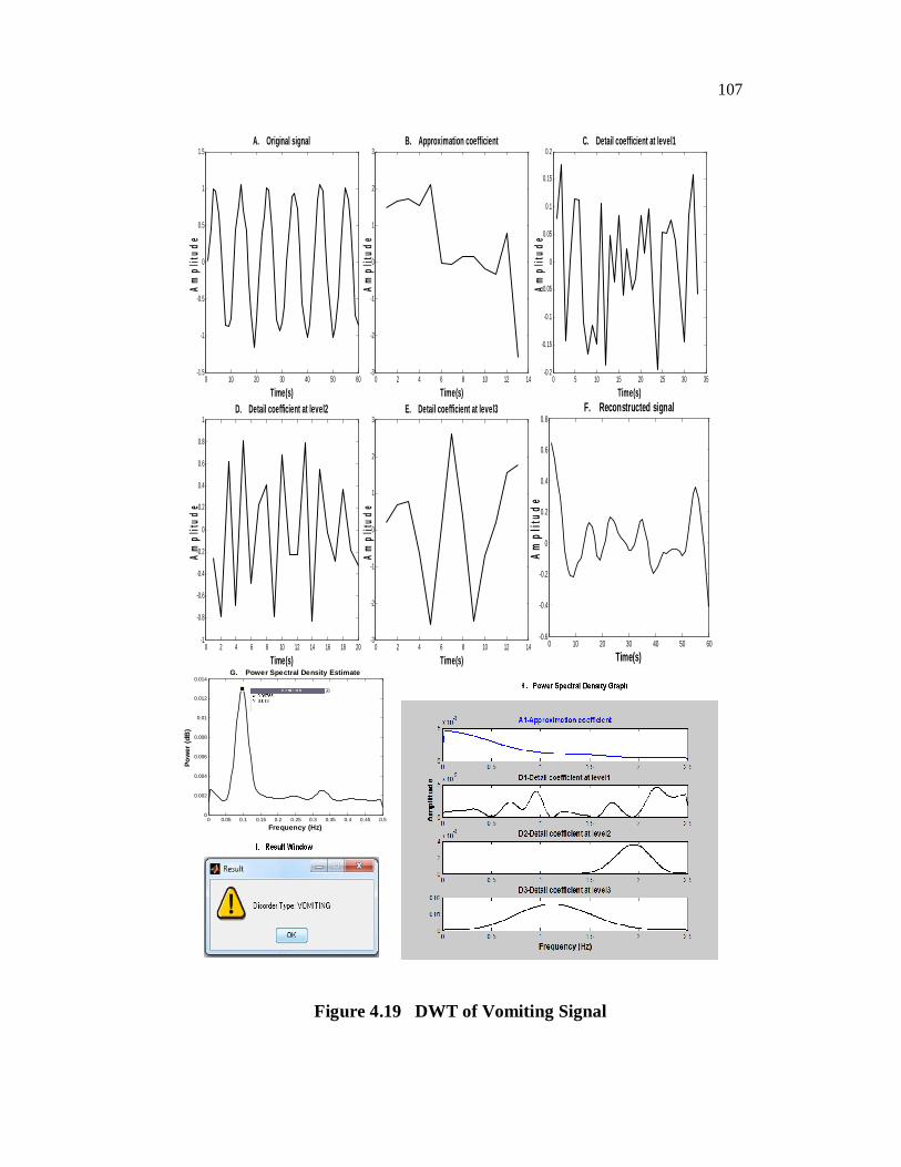
Daubechies (db4) wavelet transform is applied to the EGG signals

of normal subjects and abnormal subjects namely bradygastria, dyspepsia,

nausea, tachygastria, ulcer and vomiting. Figure 4.13 to Figure 4.19 show

original signal identified by ‘A’, third level approximation coefficients (A3)

identified by ‘B’ and details (D1-D3) as identified by ‘C’, ‘D’, ‘E’,

reconstructed signal is identified by ‘F’, power spectral estimate is identified

by ‘G’, power spectral density graph of decomposed EGG is identified by ‘H’ for

normal, bradygastria, dyspepsia, nausea, tachygastria, ulcer, and vomiting

subjects.

These approximation and detail records are reconstructed from the

wavelet coefficients. Approximation A2 is obtained by superimposing details

D3 on approximation A3. Approximation A1 is obtained by superimposing

101

details D2 on approximation A2. Finally, the reconstructed signal is obtained

by superimposing details D1 on approximation A1. ‘I’ shows the result

window which displays the type of EGG.

0 10 20 30 40 50 60-1.5

-1

-0.5

0

0.5

1

1.5

Time(s)

Am

plitu

de

A. Original signal

0 2 4 6 8 10 12 14-3

-2

-1

0

1

2

3B. Approximation coefficient

Time(s)

Am

plitu

de

0 5 10 15 20 25 30 35-0.12

-0.1

-0.08

-0.06

-0.04

-0.02

0

0.02

0.04

0.06

0.08C. Detail coefficient at level1

Time(s)

Am

plitu

de

0 2 4 6 8 10 12 14 16 18 20-0.4

-0.3

-0.2

-0.1

0

0.1

0.2

0.3

0.4

0.5D. Detail coefficient at level2

Time(s)

Am

plitu

de

0 2 4 6 8 10 12 14-1.5

-1

-0.5

0

0.5

1

1.5

2E. Detail coefficient at level3

Time(s)

Am

plitu

de

0 0.05 0.1 0.15 0.2 0.25 0.3 0.35 0.4 0.45 0.50

0.002

0.004

0.006

0.008

0.01

0.012

0.014G. Power Spectral Density Estimate

Frequency (Hz)

Pow

er (d

B)

0 10 20 30 40 50 60-1.5

-1

-0.5

0

0.5

1

1.5F. Reconstructed signal

Time(s)

Ampl

itude

Figure 4.13 DWT of Normal EGG

102

0 0.05 0.1 0.15 0.2 0.25 0.3 0.35 0.4 0.45 0.50

0.001

0.002

0.003

0.004

0.005

0.006

0.007

0.008

0.009


Frequency (Hz)

Pow

er (d

B)

0 10 20 30 40 50 60-1.5

-1

-0.5

0

0.5

1

1.5

Time(s)

Am

plitu

de

A. Original signal

0 2 4 6 8 10 12 14-3

-2

-1

0

1

2


Time(s)A

mpl

itude

0 5 10 15 20 25 30 35-0.6

-0.4

-0.2

0

0.2

0.4

0.6


Time(s)

Am

plitu

de

0 2 4 6 8 10 12 14 16 18 20-1

-0.8

-0.6

-0.4

-0.2

0

0.2

0.4

0.6


Time(s)

Am

plitu

de

0 2 4 6 8 10 12 14-0.6

-0.4

-0.2

0

0.2

0.4

0.6

0.8

1

1.2E. Detail coefficient at level3

Time(s)

Am

plitu

de

0 10 20 30 40 50 60-1

-0.5

0

0.5

1


Time(s)

Am

plitu

de

Figure 4.14 DWT of Bradygastria Signal .

103

0 10 20 30 40 50 60-1.5

-1

-0.5

0

0.5

1

1.5

Time(s)

Am

plitu

de

A. Original signal

0 2 4 6 8 10 12 14-2.5

-2

-1.5

-1

-0.5

0

0.5

1

1.5

2

2.5B. Approximation coefficient

Time(s)

Am

plitu

de0 5 10 15 20 25 30 35

-0.2

-0.15

-0.1

-0.05

0

0.05

0.1


Time(s)

Am

plitu

de

0 2 4 6 8 10 12 14 16 18 20-0.8

-0.6

-0.4

-0.2

0

0.2

0.4


Time(s)

Am

plitu

de

0 2 4 6 8 10 12 14-1.5

-1

-0.5

0

0.5

1

1.5E. Detail coefficient at level3

Time(s)

Am

plitu

de

0 0.05 0.1 0.15 0.2 0.25 0.3 0.35 0.4 0.45 0.50

0.002

0.004

0.006

0.008

0.01


Frequency (Hz)

Pow

er (d

B)

0 10 20 30 40 50 60-1.5

-1

-0.5

0

0.5

1


Time(s)

Am

plitu

de

Figure 4.15 DWT of Dyspepsia Signal

104

0 0.05 0.1 0.15 0.2 0.25 0.3 0.35 0.4 0.45 0.50

0.005

0.01


Frequency (Hz)

Pow

er (d

B)

0 2 4 6 8 10 12 14-4

-3

-2

-1

0

1

2

3


Time(s)

Am

plitu

de

0 2 4 6 8 10 12 14 16 18 20-1.5

-1

-0.5

0

0.5

1

1.5

2D. Detail coefficient at level2

Time(s)

Am

plitu

de

0 5 10 15 20 25 30 35-1.5

-1

-0.5

0

0.5

1C. Detail coefficient at level1

Time(s)

Am

plitu

de

0 2 4 6 8 10 12 14-1

-0.5

0

0.5

1

1.5

2

2.5

3


Time(s)A

mpl

itude

0 10 20 30 40 50 60-2

-1.5

-1

-0.5

0

0.5

1

1.5

2

Time(s)

Am

plitu

de

A. Original signal

0 10 20 30 40 50 60-2

-1.5

-1

-0.5

0

0.5

1

1.5

2F. Reconstructed signal

Time(s)

Ampl

itude

Figure 4.16 DWT of Nausea Signal

105

0 0.05 0.1 0.15 0.2 0.25 0.3 0.35 0.4 0.45 0.50

0.002

0.004

0.006

0.008

0.01

0.012


Frequency (Hz)

Pow

er (d

B)

0 10 20 30 40 50 60-2

-1.5

-1

-0.5

0

0.5

1

1.5

2

2.5

Time(s)

Am

plitu

de

A. Original signal

0 2 4 6 8 10 12 14-1.5

-1

-0.5

0

0.5

1

1.5

2

2.5

3


Time(s)

Am

plitu

de0 5 10 15 20 25 30 35

-1

-0.8

-0.6

-0.4

-0.2

0

0.2

0.4

0.6

0.8


Time(s)

Am

plitu

de

0 2 4 6 8 10 12 14 16 18 20-2

-1.5

-1

-0.5

0

0.5

1


Time(s)

Am

plitu

de

0 2 4 6 8 10 12 14-3

-2

-1

0

1

2

3


Time(s)

Am

plitu

de

0 10 20 30 40 50 60-0.8

-0.6

-0.4

-0.2

0

0.2

0.4

0.6

0.8


Time(s)

Am

plitu

de

Figure 4.17 DWT of Tacygastria Signal

106

0 10 20 30 40 50 60-3

-2

-1

0

1

2

3

Time(s)

Am

plitu

de

A. Original signal

0 2 4 6 8 10 12 14-2

-1.5

-1

-0.5

0

0.5

1

1.5

2

2.5


Time(s)

Am

plitu

de0 5 10 15 20 25 30 35

-2

-1.5

-1

-0.5

0

0.5

1

1.5


Time(s)

Am

plitu

de

0 2 4 6 8 10 12 14 16 18 20-2

-1.5

-1

-0.5

0

0.5

1


Time(s)

Am

plitu

de

0 2 4 6 8 10 12 14-3

-2

-1

0

1

2

3

4


Time(s)

Am

plitu

de

0 0.05 0.1 0.15 0.2 0.25 0.3 0.35 0.4 0.45 0.50

0.002

0.004

0.006

0.008

0.01

0.012

0.014


Frequency (Hz)

Pow

er (d

B)

0 10 20 30 40 50 60-2.5

-2

-1.5

-1

-0.5

0

0.5

1

1.5


Time(s)

Am

plitu

de

Figure 4.18 DWT of Ulcer Signal

107

0 10 20 30 40 50 60-1.5

-1

-0.5

0

0.5

1

1.5

Time(s)

Am

plitu

de

A. Original signal

0 5 10 15 20 25 30 35-0.2

-0.15

-0.1

-0.05

0

0.05

0.1

0.15


Time(s)

Am

plitu

de

0 2 4 6 8 10 12 14-3

-2

-1

0

1

2


Time(s)

Am

plitu

de

0 2 4 6 8 10 12 14 16 18 20-1

-0.8

-0.6

-0.4

-0.2

0

0.2

0.4

0.6

0.8

1D. Detail coefficient at level2

Time(s)

Am

plitu

de

0 2 4 6 8 10 12 14-3

-2

-1

0

1

2


Time(s)

Am

plitu

de

0 0.05 0.1 0.15 0.2 0.25 0.3 0.35 0.4 0.45 0.50

0.002

0.004

0.006

0.008

0.01

0.012


Frequency (Hz)

Pow

er (d

B)

0 10 20 30 40 50 60-0.6

-0.4

-0.2

0

0.2

0.4

0.6


Time(s)

Am

plitu

de

Figure 4.19 DWT of Vomiting Signal

108

Table 4.6 represents the threshold levels for different symptoms in

EGG by computing Mean square error between the original and the

reconstructed signal (Jaffery et al 2010). This table is used as reference for

formation of confusion matrix.

Table 4.6 MSE range for different EGG

Sl. No. EGG Threshold Range

1 Normal 0.0221-0.0425

2 Bradygastria 0.0077-0.0217

3 Dyspepsia 0.0514-0.0520

4 Nausea 0.0426-0.0513

5 Tachygastria 0.0527-0.0593

6 Ulcer 0.0608-0.0755

7 Vomiting 0.0594-0.0607

4.4.2 Confusion Matrix for DWT

Confusion matrix formed for the signals acquired in the laboratory

setup with different composition as in Table 3.5 are tabulated in Table 4.7 and

Table 4.8 for different sample sets.

109

Table. 4.7 Confusion matrix generated using DWT for 200 and 300 Samples


Predicted

Classes


13.0 0.0 0.0 1.0 1.0 0.0 1.0 13.0 0.0 0.0 1.0 0.0 0.0 0.0

1.0 30.0 0.0 1.0 0.0 1.0 1.0 1.0 48.0 1.0 2.0 0.0 0.0 0.0

1.0 0.0 24.0 2.0 0.0 1.0 0.0 0.0 3.0 46.0 0.0 2.0 2.0 2.0

0.0 2.0 2.0 29.0 0.0 1.0 0.0 0.0 0.0 5.0 37.0 0.0 0.0 0.0

0.0 0.0 0.0 3.0 27.0 1.0 2.0 1.0 2.0 1.0 2.0 46.0 2.0 0.0

1.0 1.0 2.0 0.0 1.0 31.0 0.0 1.0 2.0 2.0 1.0 2.0 44.0 1.0

1.0 0.0 0.0 0.0 1.0 1.0 16.0 0.0 1.0 1.0 2.0 1.0 1.0 24.0

110

Table. 4.8 Confusion matrix generated using DWT for 400 and 500 Samples


Predicted

Classes


33.0 0.0 1.0 1.0 1.0 1.0 0.0 39.0 0.0 1.0 0.0 1.0 3.0 0.0

0.0 52.0 1.0 2.0 3.0 3.0 1.0 1.0 68.0 1.0 3.0 2.0 2.0 0.0

0.0 4.0 61.0 0.0 3.0 2.0 1.0 2.0 5.0 59.0 2.0 1.0 0.0 0.0

0.0 2.0 3.0 55.0 0.0 2.0 0.0 5.0 1.0 4.0 76.0 3.0 5.0 0.0

3.0 1.0 4.0 4.0 58.0 0.0 1.0 1.0 3.0 2.0 3.0 72.0 0.0 1.0

0.0 1.0 1.0 1.0 0.0 55.0 2.0 0.0 2.0 2.0 1.0 2.0 86.0 1.0

0.0 0.0 0.0 2.0 0.0 3.0 32.0 0.0 0.0 1.0 2.0 0.0 2.0 35.0

111

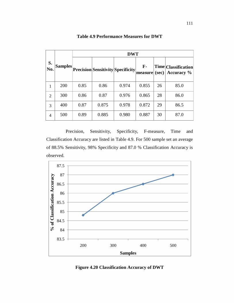
Table 4.9 Performance Measures for DWT

S. No.

Samples

DWT

Precision Sensitivity Specificity F-

measure Time (sec)

Classification Accuracy %

1 200 0.85 0.86 0.974 0.855 26 85.0

2 300 0.86 0.87 0.976 0.865 28 86.0

3 400 0.87 0.875 0.978 0.872 29 86.5

4 500 0.89 0.885 0.980 0.887 30 87.0

Precision, Sensitivity, Specificity, F-measure, Time and

Classification Accuracy are listed in Table 4.9. For 500 sample set an average

of 88.5% Sensitivity, 98% Specificity and 87.0 % Classification Accuracy is

observed.

Figure 4.20 Classification Accuracy of DWT

83.5

84

84.5

85

85.5

86

86.5

87

87.5

200 300 400 500

% o

f Cla

ssifi

catio

n A

ccur

acy

Samples

112

1.5 CONCLUSION

In this chapter, Continuous Wavelet Transform and Discrete

Wavelet Transform analysis is performed on EGG signals to detect the

disorders. This study shows that it is possible to show significant difference

between subjects who are normal and dysarrhythmic. Chacon et al (2009)

used NN classifier using wavelet coefficient for healthy and dyspepsia

subjects and has reported 78.6% Sensitivity, 92.9% Specificity and 82.1%

Classification Accuracy. The DWT based approach used in this thesis gave

88.5% Sensitivity, 98 % Specificity and 87% Classification Accuracy,

whereas in CWT 83.5% Sensitivity, 97 % Specificity and 82.5%

Classification Accuracy were observed. Based on the investigation carried out

in this chapter it is found that DWT method is very useful in the analysis of

EGG recordings especially in detecting normal events and arrhythmic in

EGG.

Investigation carried out using wavelet transform show 5%, 0.4%

improvement in classification with DWT and CWT respectively when

compared with Chacon et al (2009).

Documents

CHAPTER 4 WAVELET ANALYSIS OF …shodhganga.inflibnet.ac.in/bitstream/10603/16353/9/09_chapter4.pdf · CHAPTER 4 WAVELET ANALYSIS OF ELECTROGASTROGRAM SIGNALS 4.1 INTRODUCTION Biosignals