65

Chapter 4. Vibrational and Rotational States Notes: • Most of the material presented in this chapter is taken from Bunker and Jensen

(2005), Chaps. 4 and 5, Bunker and Jensen (1998), Chap. 11, and Kroto1, Chap. 3.

4.1 Vibrational States From equation (3.107) we can write the quantum mechanical harmonic oscillator Hamiltonian to be

Hvib0 =

12

Pk2 + !kQk

2( )k=1

3N "6

# , (4.1)

which is one part of the more general vibrational Hamiltonian Hvib = Hvib

0 +VN,nanh . (4.2)

For what will follow, we will mainly focus on the harmonic oscillator approximation with equation (4.1).

4.1.1 The Non-degenerate Harmonic Oscillator In cases where all the eigenvalues !k are different (i.e., there is no degeneracy) the Hamiltonian is composed of 3N ! 6 independent harmonic oscillators, thus its name. The one-dimensional harmonic oscillator wave equation is given by

Hho ! =12P2 + "Q2( ) ! = E! ! , (4.3)

where we will write !" Q( ) = Q " for the wave (eigen)function of energy (eigenvalue) E! . It will be useful for the analysis that follows to introduce the following operators

R± =12P ± i!1 2Q( ). (4.4)

It is also interesting to calculate the commutators

Hho ,R±!" #$ =

12 2

±i%1 2 P2 ,Q!" #$ + % Q2 , P!" #${ }=

12 2

±i%1 2 &2i!P( ) + % 2i!Q( ){ } = ±!%1 2R± . (4.5)

1 Kroto, H. W. 1992, Molecular Rotation Spectra (New York: Dover).

66

Because of this relation, it is easy to show that

Hho R± !( ) = E! ± !"

1 2( ) R± ! . (4.6) This implies that R± ! is also an eigenvector of the Hamiltonian, but this new eigenvector has its energy level shifted by ±!!

1 2 from that of ! . For this reason

R+ and R! are called ladder operators. As will be shown below, starting with any ket ! we can span the whole set of eigenvectors by successive application of R+ and R! .

The Hamiltonian can also be expressed as a function of the operators with

Hho = R

± R! ±12"!1 2 . (4.7)

In order to identify the set of eigenvectors and their associated energy levels, we need to determine ! (or !1 2 ). To do so, let’s consider the following relation

!"# Q( ) R± R!( )!" Q( )dQ$ = R!!" Q( )%& '(

#R!!" Q( )%& '(dQ$

= R!!" Q( ) 2 dQ$ > 0, (4.8)

which implies that R± R! is Hermitian with real and positive eigenvalues. Since the Hamiltonian is also Hermitian with real eigenvalues, we deduce from equation (4.7) that !1 2 (and by the same token ! ) must be real. We further define !1 2 to be positive, as this is equivalent to defining R+ and R! in equations (4.4). It is therefore apparent from equation (4.7) that the eigenvalues of the Hamiltonian are not only real, but also positive. We will denote the minimum energy value by E0 with an associated wave function !0 Q( ) , and since R! decreases the energy we must have

R!"0 Q( ) = 1

2!i! #

#Q! i$1 2Q

%&'

()*"0 Q( ) = 0. (4.9)

This first order differential equation can be solved to give (with a given convention for normalization)

!0 Q( ) = "1 2

#!$%&

'()

1 4

e*"1 2Q2

2! . (4.10)

It is costmary to set !

1 2 " !# , so that

67

!0 Q( ) = "#

$%&

'()1 4

e*"Q2

2 . (4.11)

Furthermore, with the combination of equations (4.7) and (4.9) we have

R+ R!"0 Q( )#$ %& = Hho !

12!2'(

)*+,-"0 Q( ) = 0, (4.12)

and

E0 =

12!2! . (4.13)

Since from equation (4.6) every application of R+ on !0 Q( ) will increase the energy by

!2! , then we find that

E! = ! +

12

"#$

%&'!2( . (4.14)

In a similar fashion, given a wave vector ! we can determine ! ±1 with ! !1 = N! R

! ! , (4.15) where N! is normalization factor to be determined. To do so we consider

! !1! !1 = N!2! R± R! !

= N!2! Hvib

0 !12"2"#

$%&'( !

= N!2! + 1

2!12

#$%

&'( "

2"

= 1,

(4.16)

where equation (4.7) was used for the second step. The normalization factor N± can easily be determined with this equation. The choice of the phase for N± is usually chosen so that

N± = !i ! +

12±12

"#$

%&'"2()

*+,-.

/1 2

. (4.17)

68

With this result and starting with equation (4.11), while using equations (4.4), one can show that

!" Q( ) = N"H" # 1 2Q( )e$#Q2

2 , (4.18) where

N! =" 1 4

2!# 1 2!! (4.19)

and H! " 1 2Q( ) are the so-called Hermite polynomials. For example, it can be shown that

H0 ! 1 2Q( ) = 1H1 ! 1 2Q( ) = 2! 1 2QH2 ! 1 2Q( ) = 4!Q2 " 2

H 3 ! 1 2Q( ) = 8! 3 2Q3 "12! 1 2Q,

(4.20)

and so on. In summary, for a molecule, whose vibrational Hamiltonian (with no degeneracy) is given by

Hvib0 =

12

Pk2 + !kQk

2( )k=1

3N "6

# , (4.21)

the wave functions associated with this Hamiltonian are given by

!vib = !"1Q1( )!"2

Q2( )!!"3N#6Q3N #6( )

= exp #12

$ jQj2

j=1

3N #6

%&

'()

*+N"k

H"k$ k1 2Q( )

k=1

3N #6

, , (4.22)

with corresponding energy levels

Evib = !k +

12

"#$

%&'!2( k

k=1

3N )6

* . (4.23)

It is important to realize that if such a molecule were left on its own (i.e., there are no perturbations to the Hamiltonian), then the wave functions representing its states would never mix. This is because these wave functions form the basis that diagonalizes the Hamiltonian. That is, if we calculate the elements of the Hamiltonian “matrix” we find that

69

! Hvib

0 "! = E "! ! "! = E "! #! "! . (4.24) This result shows that there are no elements “off the diagonal of the matrix”, and there are therefore no interaction between the different states. But of course, this is a highly idealized situation. For example, using the more general vibrational Hamiltonian of equation (4.2) we find that

! Hvib "! = ! Hvib

0 +VN,nanh( ) "!

= E "! #! "! + ! VN,nanh "! .

(4.25)

Therefore, depending on the exact nature of VN,n

anh it is possible that the last term on the right hand side of this equation be not zero, even when ! " #! . Let’s consider the simple case of a molecule that has only one normal mode of vibration, and where the anharmonic potential (a perturbation) can be approximated by VN,n

anh = aQ3, (4.26) with a some constant. To see the effect that this cubic term has on the molecule we will need to consider the following expression (easily derived from equations (4.4))

Q =

12i!!

R+ " R"( ). (4.27)

Incidentally, it is also true that

P =12R+ + R!( ). (4.28)

We now use the completeness relation twice (see equation (1.16)) to calculate

! VN,n

anh "! = a ! Q3 "!

= a ! Q µ µ Q # # Q "!µ ,#$ , (4.29)

which we further transform with the information contained in equation (4.27)

! VN,nanh "! = a ! Q ! #1 ! #1 Q ! # 2 ! # 2 Q "!$%

+ ! Q ! #1 ! #1 Q ! ! Q "!+ ! Q ! +1 ! +1 Q ! ! Q "!

+ ! Q ! +1 ! +1 Q ! + 2 ! + 2 Q "! &'.

(4.30)

70

This shows that the states satisfying the conditions ! " 2 = #! ±1 , ! = "! ±1, or ! + 2 = "! ±1 (or alternatively ! = "! ±1 or ! = "! ± 3 ) can mix. As will be emphasized in later chapters, this is the basic process through which a molecule changes states. For example, the interaction of molecule with a radiation field will be modeled by introducing a perturbation Hamiltonian that will connect different states in a manner similar to what was detailed with equations (4.29) and (4.30). If a molecule absorbs a photon, it must make a transition from its initial state to a final state that will satisfy mixing relations (the so-called selection rules) established by the detailed nature of the perturbation (or interaction) Hamiltonian.

Finally, it can be shown that the non-vanishing matrix elements of Q and P are

! +1Q ! = ! +1( ) 2"( ), ! +1 P ! = i! ! +1( )" 2,

! #1Q ! = ! 2"( ), ! #1 P ! = #i! !" 2. (4.31)

4.1.2 The Two-dimensional (Degenerate) Harmonic Oscillator

If it happens that two eigenvectors !a and !b of a harmonic oscillator have a common energy such that ! a = ! b " ! , then it is not possible to completely specify the states of the system using only its total energy. That is, the total energy of this two-dimensional oscillator is given by

E !a ,!b( ) = !a +

12

"#$

%&'+ !b +

12

"#$

%&'

()*

+,-!2. , (4.32)

and it is clear that

E 0,1( ) = E 1,0( ) = 2!2!E 0,2( ) = E 1,1( ) = E 2,0( ) = 3!2! ,

(4.33)

and so on. Continuation of this process would show that each energy level has degeneracy of !a +!b +1( ) . The complete specification of the state of the oscillator would require the knowledge both !a and !b .

On the other hand, we are not restricted to using these two quantum numbers. We could introduce different coordinates to formulate the problem, along the appropriate eigenvectors, and labels needed to specify the state of the oscillator. To make this clearer, consider the new coordinates Q and ! such that

Qa = Qcos !( )Qb = Qsin !( ). (4.34)

71

For what will follow, it will be necessary to express the two-dimensional harmonic oscillator Hamiltonian H tdho with these coordinates. Since Q and ! are basically ordinary polar coordinates, it should be clear that in coordinate space

P2 = Pa2 + Pb

2 = !!2" #"

= !!2$2

$Q2 +Q!1 $$Q

+ Q!1( )2 $2

$% 2

&

'(

)

*+

Vtdho =12!2, 2 Qa

2 +Qb2( ) = !2, 2Q2 ,

(4.35)

and therefore

H tdho =

!2

2!

"2

"Q2 +Q!1 ""Q

+ Q!1( )2 "2

"# 2

$

%&

'

() + *

2Q2+,-.

/01.. (4.36)

The new states we are seeking must still be eigenvectors for this Hamiltonian, and will have a quantum number, say, ! , associated with them. From equation (4.32) we can write E! = ! +1( )!2" , (4.37) or ! = !a +!b = 0,1,2,… . We would like to find another operator that would share the same set of eigenvectors with H tdho , and therefore commutes with it, to which we could attach a new label, say, l . The idea is that specifying ! and l would completely determine the state of the oscillator. Consider the following operator (making use of the chain rule)

M = !i! ""#

= !i! "Qa

"#"

"Qa

+"Qb

"#"

"Qb

$%&

'()

= !i! !Qsin #( ) ""Qa

+Qcos #( ) ""Qb

*

+,

-

./

= QaPb !QbPa ,

(4.38)

which has the units of a vibrational angular momentum operator. Because of its simple form (i.e., M = !i!" "# ), it is obvious that this operator commutes with H tdho (as expressed through equation (4.36)). We can therefore write, with !,l the new eigenvectors,

72

H tdho !,l = ! +1( )!2" !,l

M !,l = l! !,l , (4.39)

where the vibrational angular quantum number l still needs to be suitable defined. However, because of the last of equations (4.39) it is already possible to assess that

!" ,l Q,#( ) = Q,# ",l

= F" ,l Q( )eil# , (4.40)

where F! ,l Q( ) is a function of Q only. If we use the usual definition for the momentum, i.e.,

P = !i! "

"Q, (4.41)

and further introduce

Q± = Qa ±Qb = Qe

± i!

P± = Pa ± Pb = e± i! P ± iQ"1M( ), (4.42)

then we can write

H tdho =12P2 ! i!Q!1P +Q!2M + !2" 2Q2( )

=12P+P! + !2" 2Q+Q!( ).

(4.43)

In a manner similar to what was done for the non-degenerate case, ladder operators can be defined with

R± ±( ) = e ±( )i! P ± i!"Q ±( )iQ#1M$% &'= P ±( ) ± i!"Q ±( )

(4.44)

where the ± and ±( ) are respectively correlated on either side of the equality sign. There are, therefore, four different ladder operators. It is not too difficult to derive the following commutation relations

H tdho , R± ±( )!" #$ = ±!2% R± ±( )

M , R± ±( )!" #$ = ±( )!R± ±( ), (4.45)

73

which implies that the operators have the following effect on the quantum numbers for the energy and the vibrational angular momentum R± ±( ) : transforms ! "! ±1 and l" l ±( )1. (4.46) Using a technique akin to the one used for the one-dimensional harmonic oscillator, it also possible to show that

! 0,0 Q( ) = "

#e$"Q2

2

!% ,l Q,&( )' R+ $( )() *+%$ l( ) 2

R+ +( )() *+%+ l( ) 2

! 0,0 Q( ), (4.47)

with l = !,! " 2,…,"! . The different states can be coupled by the normal coordinates and momenta operators through the ladder operators, as can be asserted using the following relations

Qa =

12Q+ +Q!( ), Qb =

12i

Q+ !Q!( ),

Pa =12P+ + P!( ), Pb =

12i

P+ ! P!( ), (4.48)

and

Q ±( ) =12i!!

R± ±( ) " R" ±( )#$ %&

P ±( ) =12R± ±( ) + R" ±( )#$ %&.

(4.49)

For the sake of completeness we will state that in the case of a triply degenerated normal mode the wave functions are specified with three quantum numbers !" ,l ,n Q,#,$( ) ( l and n are vibrational quantum numbers related to the ! and " angles, respectively), while the energy is given by

E! = ! +

32

"#$

%&'!2( , (4.50)

where ! = 0,1,2,… . Finally, the other two quantum numbers take the values

l = !,! " 2,! " 4, …,1 or 0n = "l,"l +1, …,l "1,l.

(4.51)

74

Figure 4-1 – The energy vibration levels for four molecules.

Using the results from the analyses performed in this section, it is possible to plot the vibrational energy levels for molecules in the harmonic oscillator approximation. A few examples are shown in Figure 4-1. Note that the levels are regularly spaced when there is only one normal mode (see equation (4.14)), as is the case for CO, but the spectra take a much more convoluted appearance when more than one mode are present.

4.2 Rotational States From equation (3.107), we can write the quantum mechanical rigid rotator Hamiltonian to be

H rot

0 =12

µ!!e J!

2

!"

= Ae Ja2 + Be Jb

2 + Ce Jc2 ,

(4.52)

where

Ae =12Iaa

e , Be =12Ibb

e , and Ce =12Icc

e . (4.53)

The principal axes a, b, and c (in the equilibrium configuration using the molecular-fixed coordinate system) are always defined such that Ae ! Be ! Ce , and whether the molecular fixed z-axis is identified with the a, b, and c index the situation is usually defined as

75

type I, II, or III. A r or l superscript can be added to the type depending if one works with a right or left handed coordinate system; we will only consider right handed systems.

4.2.1 Space-fixed Angular Momentum We have already discussed the space-fixed angular momentum operators in Chapter 1, as well as some of their commutation properties. So, given J! , J" , and J# we have

J j , Jk!" #$ = i!% jkl Jl , (4.54)

with j, k, l = !, ", or # . We also know that J 2 , the square of the total orbital angular momentum, possesses the following commutation relations J 2 , Jk!" #$ = 0, (4.55) which implies that it will be possible to set up rotational wave functions !rot that will be simultaneous eigenfunctions of J 2 and J! (we could have chosen J! or J! instead of

J! , but it is the convention to chose the latter). We will, for the moment, denote the kets

associated with these wave functions by J 2 ,m , where J 2!2 and m! are the eigenvalues

of J 2 and J! , respectively.

We now introduce the operators Js

± = J! ± iJ" , (4.56) for which the following commutation relations can easily be established

J! , Js

±"# $% = ±!Js± . (4.57)

Using equation (4.57) we can calculate that

J! Js± J 2 ,m = Js

± J! ± !Js±( ) J 2 ,m

= m ±1( )!Js± J 2 ,m , (4.58)

which implies that whenever Js

± acts on a eigenvector it transforms it to another eigenvector of eigenvalue m ±1( )! . It is therefore apparent that Js

± are ladders operators that will allow us to span the whole set of eigenvectors associated to a given eigenvalue J 2!2 . Moreover, we deduce that m must have lower and upper bounds, since the following relation must be obeyed

76

m! ! J 2!2 . (4.59) If we denote the upper and lower bounds of m as m+ and m! , respectively, then we can write Js

± J 2 ,m± = 0. (4.60) Furthermore, we have

Js! Js

± J 2 ,m± = J!2 + J"

2 ± i J! , J"#$ %&( ) J 2 ,m±

= J 2 ' J(2 ! "J(( ) J 2 ,m±

= J 2 ' m±2 ! m±( )"2 J 2 ,m±

= 0.

(4.61)

From this result we obtain the two equations

J 2 ! m!

2 + m! = 0J 2 ! m+

2 ! m+ = 0, (4.62)

from which we can take the difference, and transform it to m+ + m!( ) m+ ! m! +1( ) = 0. (4.63) The term within the second set of parentheses must be greater than zero because m+ ! m" , which implies that the term within the first set of parentheses must cancel and

m+ = !m!

m+ ! m! = 2 j, (4.64)

where 2 j has to be some positive integer number, since m+ !m! corresponds to the number of times (i.e., 2 j times) Jm

± is applied to J2,m! to span the whole set of kets.

It is now clear from equations (4.62) and (4.64) that m+ = j and J 2 = j j +1( ). (4.65) Furthermore, the second of equation (4.64) tell us that m is quantized and can either be integer or half-integer, so that m = j, j !1,…,1,0,!1,…,! j (4.66)

77

or

m = j, j !1,…, 1

2,! 12,…,! j. (4.67)

It can be shown, using equations (3.1), (3.2), and (3.73), that the angular momentum operators take the following form in coordinate space

J! = "i! cos #( ) " cot $( ) %%#

+1

sin $( )%%&

'

()

*

+, " sin #( ) %

%$-./

0/

12/

3/

J4 = "i! sin #( ) " cot $( ) %%#

+1

sin $( )%%&

'

()

*

+, + cos #( ) %

%$-./

0/

12/

3/

J5 = "i! %%#

Js± = "i!e± i# " cot $( ) %

%#+

1sin $( )

%%&

±%%$

'

()

*

+,

J 2 = "!21

sin $( )%%$

sin $( ) %%$

'()

*+,+

1sin2 $( )

%2

%# 2+

%2

%& 2 " 2cos $( ) %2

%#%&'

()

*

+,

-.0/

123/.

(4.68)

4.2.2 Molecule-fixed Angular Momentum Since the rotation Hamiltonian of equation (4.52) is expressed using the molecule-fixed coordinates x, y and z , it is also important to derive the commutation relations for the angular momentum operators expressed in this coordinate system. Furthermore, the wave functions associated with the Hamiltonian are a function of the three Euler angles; we will then require one more operator besides J 2 and J! (which commutes with J 2 ) to completely specify the state of rotation of the molecule. Because we know from equations (4.68) that J 2 depends on all three angles, while J! is a function of only ! , we will benefit from using an operator with the simplest dependency, i.e., either on ! or ! . We will, therefore, make the educated guess that a good operator for this task is Jz , as will be justified by our analysis. Because the molecule-fixed components of the angular momentum operators can be expressed as a linear combination of the space-fixed components through the Euler matrix (see equations (3.1) and (3.2)), it is straightforward to show, from equation (4.55), that J 2 , Jk!" #$ = 0, (4.69)

78

with k = x, y, or z . On the other hand, careful use of the same transformation relations between the molecule- and space-fixed angular momentum components will yield the following commutation relations

J j , Jk!" #$ = %i!& jkl Jl , (4.70)

where j, k, l = x, y, or z . Take notice of the sign difference on the right hand side of equations (4.54) and (4.70). Just as was previously done for the space-fixed operators we introduce the ladder operators Jm

± = Jx ± iJy , (4.71) for which the following commutation relations can easily be established

Jz , Jm

±!" #$ = !"Jm± . (4.72)

Again, take note of the sign difference relative to equation (4.57). Going through the same process that was used for the space-fixed operators we find that we can add a new quantum number k to define the eigenvectors such that Jz J,k,m = k! J,k,m , (4.73) where we have also replaced J 2 by J in the ket to specify the eigenvalue of J 2 (that of J! , i.e., m , is unchanged). Also, because of the sign difference of equations (4.70) and (4.72) we find that the roles of the ladder operators are inverted. That is, we now have Jz Jm

± J,k,m = k !1( )"Jm± J,k,m . (4.74) Note that k covers the same range of values as m does (see equations (4.66) and (4.67), with j! J ). It can be shown, using equations (3.73), that the angular momenta operators take the following form in coordinate space

Jx = !i! cos "( ) cot #( ) $$"

!1

sin #( )$$%

&

'(

)

*+ + sin "( ) $

$#,-.

/.

01.

2.

Jy = i! sin "( ) cot #( ) $$"

!1

sin #( )$$%

&

'(

)

*+ ! cos "( ) $

$#,-.

/.

01.

2.

Jz = !i!$$",

(4.75)

79

and

Jm± = i!e" i! " cot #( ) $

$%+

1sin #( )

$$!"

$$#

&

'(

)

*+

J 2 = "!21

sin #( )$$#

sin #( ) $$#

&'(

)*++

1sin2 #( )

$2

$! 2+

$2

$% 2 " 2cos #( ) $2

$!$%&

'(

)

*+

,-./

012/. (4.76)

Finally, we write down the matrix elements for some of the angular momentum operators (space- and molecular-fixed)

J,k,m J 2 J,k,m = J J +1( )!2

J,k,m Jz J,k,m = k!

J,k "1,m Jm± J,k,m = ! J J +1( ) ! k k "1( )

J,k,m J" J,k,m = m!

J,k,m ±1 Js± J,k,m = ! J J +1( ) ! m m ±1( ).

(4.77)

4.2.3 The Eigenfunctions of the Angular Momentum Operators We will define the eigenfunctions of the angular momentum operators in coordinate space with

!rot ",#,$( ) = ",#,$ J,k,m

= %Jkm "( )!m #( )&k $( ), (4.78)

where the last equation indicates that we are expecting to obtain a solution through a separation of the variables. As a first step, we note that applying J! and Jz (see the third of equations (4.68) and (4.75)) to equation (4.78) will simply yield

!i! ""#

$m #( ) = m!$m #( )

!i! ""%

&k %( ) = k!&k %( ), (4.79)

with the results that (including normalization)

!m "( ) = 12#

eim" , $k %( ) = 12#

eik% . (4.80)

80

With these equations, and the application of J 2 to the eigenfunctions using the last of equations (4.76) we get

!1

sin "( )##"

sin "( ) ##"

$%&

'()!

m2 + k2 ! 2mk cos "( )$% '(sin2 "( )

*+,

-,

./,

0,1Jkm "( ) = J J +1( )1Jkm "( ). (4.81)

We could attempt to solve this equation as it stands, but it is simpler to first solve it for k = m = 0 and then apply J! and Jz to find the more general expressions for arbitrary values of k and m . Therefore, setting x = cos !( ) and k = m = 0 in equation (4.81) we are left with the so-called Legendre equation

1! x2( ) d2

dx2! 2x d

dx+ J J +1( )"

#$

%

&'(J 0 0 x( ) = 0, (4.82)

for which the Legendre polynomials PJ x( ) are the solution. In our case we have

!J 0 0 cos "( )#$ %& = J + 12PJ cos "( )#$ %&. (4.83)

For example, here are the first four Legendre polynomials

P0 cos !( )"# $% = 1

P1 cos !( )"# $% = cos !( )

P2 cos !( )"# $% =123cos2 !( ) &1"# $%

P3 cos !( )"# $% =125cos3 !( ) & 3cos !( )"# $%.

(4.84)

The successive application of J! and Jz yields

J,k,m = !N+ Jm"( )k Js

+( )m J,0,0

J,"k,"m = !N" Jm+( )k Js

"( )m J,0,0

J,k,"m = !!N+ Jm"( )k Js

"( )m J,0,0

J,"k,m = !!N" Jm+( )k Js

+( )m J,0,0 ,

(4.85)

where !N± and !!N± are some positive normalization constants. Through the projection of these kets on !,",# it is found that the explicit form of the wave functions is given by

81

!rot ",#,$( ) = %Jkm "( )!m #( )&k $( )

= N '1( )( cos " 2( ))* +,2J + k'm'2(

' sin " 2( ))* +,m' k+2(

( ! J ' m ' (( )! m ' k +(( )! J + k ' (( )!(-

./0

10

230

40eim#eik$ ,

(4.86)

with

N =1

2 2!J + m( )! J " m( )! J + k( )! J " k( )! 2J +1( ). (4.87)

In equation (4.86) the range of values for the summation index ! starts from the larger of 0 and k ! m( ) , and ends at the smaller of J ! m( ) and J + k( ) . Alternatively, these

wave functions are often expressed using the so-called rotation matrices DmkJ( ) !,",#( )

with

!rot ",#,$( ) = 2J +18% 2 Dmk

J( ) ",#,$( )&' ()*. (4.88)

4.2.4 Solutions to the Rigid Rotator Hamiltonian We shouldn’t lose sight of our goal, which is to find the eigenvalues and eigenfunctions of the rigid rotator Hamiltonian of equation (4.52). That is, we want to solve H rot

0 ! rot = Erot ! rot . (4.89) As we already know, H rot

0 commutes with J 2 and J! , which implies that we will be able

to build the eigenvectors ! rot using the set of J,k,m kets as a basis. In fact, in some cases we will find that ! rot = J,k,m . This will not be true in general, however, since

H rot0 does not always commute with Jz . It follows from this that the matrix representing

H rot0 will always be diagonal in J , but not necessarily in k . A given energy of rotation

will generally be associated with a level J , and a corresponding wave function expressible as follows (with ck

J ,m some coefficients) ! rot = ck

J ,m J,k,mk" . (4.90)

It is convenient to separate this problem in different classes, which depend on the relative values of the principal moments of inertia (see equations (4.52) and (4.53), and the discussion that follows). The following types of rotators are therefore defined

82

1. Spherical tops Iaae = Ibb

e = Icce CH4

2. Symmetric tops, a) prolate Iaae < Ibb

e = Icce CH3D

b) oblate Iaae = Ibb

e < Icce H3

+, NH3

3. Linear molecules Iaae = 0, Ibb

e = Icce CO, HCN

4. Asymmetric tops Iaae < Ibb

e < Icce H2O

4.2.4.1 Spherical Top Molecules Since the principal moments of inertia are all equal for a spherical top, then Ae = Be = Ce and the Schrödinger equation becomes Be J

2 ! rot = Erot ! rot , (4.91) with Erot = BeJ J +1( )!2 . (4.92) It should also be clear that ! rot = J,k,m . (4.93) That is, the wave functions are the eigenfunctions of J 2 (as well as those of J! and Jz ).

4.2.4.2 Symmetric Top Molecules For a prolate symmetric top molecule the rigid rotor Schrödinger equation is Ae Ja

2 + Be Jb2 + Jc

2( )!"

#$ % rot = Erot % rot . (4.94)

If we choose to work with a type Ir rotor, then we identify the a, b, and c indices with z, x, and y , respectively, and equation (4.94) transforms to Be J

2 + Ae ! Be( ) Jz2"# $% & rot = Erot & rot , (4.95) remember that Ae ! Be always. It is easy to see with this last form for the Schrödinger equation that the Hamiltonian is completely defined by J 2 and Jz . It therefore commutes with both of these operators, and shares their eigenfunctions. That is, ! rot = J,k,m , (4.96) and the energy is

83

Erot = BeJ J +1( ) + Ae ! Be( )K 2"# $%!2 , (4.97)

with J = 0, 1, 2,… , K = k , and k = 0, ±1, ± 2,…, J .

In a similar manner, it can be shown that for an oblate symmetric top molecule the Schrödinger equation is Be J

2 ! Be ! Ce( ) Jz2"# $% J,k,m = Erot J,k,m , (4.98) with ! rot = J,k,m for a type IIIr rotator (i.e., we identified the a, b, and c indices with x, y, and z ) the energy is Erot = BeJ J +1( ) ! Be ! Ce( )K 2"# $%!

2 . (4.99) Unlike the case of the spherical top, the energy or rotation of a symmetric top is dependent on K ; it increases with K for a prolate molecule, while it decreases with K for an oblate molecule.

4.2.4.3 Linear Molecules Although linear molecules constitute, in a way, the simplest type of rigid rotator, there are some aspects associated with their Hamiltonian that require special attention when analyzing their rotational spectroscopy (Bunker and Jensen (1998) dedicates one full chapter to the subject). We will not deal with these details and simply treat these molecules as the extreme case of a prolate symmetrical top molecule (it turns out that this treatment is perfectly adequate). With this approximation, equations (4.95) and (4.97) become (setting Ae = 0 is adequate, as there cannot be any energy of rotation about the corresponding axis) Be J

2 ! Jz2( ) J,k,m = Erot J,k,m , (4.100)

and Erot = Be J J +1( ) ! K 2"# $%!

2 . (4.101) But the question remains as to what value(s) can K take? This question is certainly relevant since there can be no nuclear rotational contribution to the orbital angular momentum about the z-axis . Some authors will therefore set K = 0 (e.g., Kroto, op.cit.), but our analysis will be more accurate if we take into account other sources of orbital angular momentum about the axis of symmetry. It can be shown that linear molecules composed of N atoms (and therefore having 3N ! 5 vibrational degrees of freedom) have N !1 one-dimensional stretching normal modes, and N ! 2 two-dimensional bending normal modes. Such bending modes can be treated as was shown in Section 4.1.2, where the vibrational angular momentum operator

84

and quantum number were introduced (see the second of equations (4.39)). Each mode will contribute to the total vibrational angular momentum l! about the symmetry axis according to

l! = lk!

k=1

N !2

" , (4.102)

where lk! is the vibrational angular momentum associated with the kth two-dimensional bending mode. Furthermore, the total electronic angular momentum about the symmetry axis Lz can also be shown to commute with the electronic Hamiltonian H elec for a linear molecule, with the result that Lz !elec = " !elec , (4.103) where !elec an eigenvector of H elec . The total orbital angular momentum about the z-axis is therefore l + ! , and it follows that the quantum number K , as well as k , is restricted by this value. That is, k = l + !. (4.104)

4.2.4.4 Asymmetric Top Molecules The asymmetric top rotator Hamiltonian can be written

H rot

0 = ax Jx2 + byJy

2 + cz Jz2

=12ax + by( ) Jx2 + Jy2( ) + cz Jz2 + 12 ax ! by( ) Jx2 ! Jy2( ), (4.105)

where the set ax ,by ,cz{ } takes on some arrangement of Ae , Be , and Ce . For example, if

we choose the Ir type, then ax = Be , by = Ce , and cz = Ae . Equation (4.105) can be advantageously transformed to

H rot0 = ! J 2 + " Jz

2 + # Jm+( )2 + Jm

$( )2%&'

()*, (4.106)

with

85

! =12ax + by( )

" = cz #12ax + by( )

$ =14ax # by( ).

(4.107)

A comparison with equations (4.95) and (4.98) for the Hamiltonians of the symmetric tops makes it clear that the ! term destroys any potential symmetric top appearance in equation (4.106). It is obvious from the presence of Jm

± in equation (4.106) that (unlike the cases of the symmetric tops, spherical tops, and linear molecules) H rot

0 will not commute with Jz . The kets J,k,m will therefore not be the eigenvectors for the asymmetric top Hamiltonian. However, since we will want to diagonalize the Hamiltonian using suitable linear combinations of these same kets (i.e., J,k,m ), we would do well to set up the problem so as to minimize ! , or rather its ratio to ! or " , as this will reduce the amount of mixing between kets of different k values. To do so, one would go through the different choices available (i.e., the six types I

r , Il , …, IIIr , IIIl ) to find the optimum axes configuration. Using the first three of equations (4.77), it is easy to show that the non-vanishing elements of the Hamiltonian of equation (4.106) result from

J,k,m J 2 J,k,m = J J +1( )!2

J,k,m Jz2 J,k,m = k2!2

J,k " 2,m Jm±( )2 J,k,m = !2 J J +1( ) ! k "1( ) k " 2( )"# $% J J +1( ) ! k k "1( )"# $%,

(4.108)

where the quantum number k is associated to the chosen axes convention. For example, for the type Ir ( IIIr ) k! is the angular momentum about the a-axis ( c-axis ), and is therefore often written ka ( kc ). It is apparent from equations (4.108) that there are no non-vanishing elements between kets exhibiting different values of J and m , and the Hamiltonian matrix will therefore be “block-diagonal” in appearance (each block of dimension 2J +1), as shown in Figure 4-2. Moreover, only states having the same k values or k values differing by two can mix. This implies even and odd values of k will not combine. Example To make things clearer, let’s work out the energies and eigenvectors for an asymmetric top molecule using a type Ir convention for the J = 0, 1 and 2 states.

86

Figure 4-2 – The block-diagonal appearance of (part of) the asymmetric rotator Hamiltonian matrix.

Solution First, we note that in the absence of an external field (electric of magnetic) the quantum number m does not affect the energy; we will therefore omit it and write J,k for the symmetric top eigenvectors. Second, for this type of rotator the expression for the Hamiltonian is that spelled out in equation (4.106), i.e.,

H rot0 = ! J 2 + " Jz

2 + # Jm+( )2 + Jm

$( )2%&'

()*, (4.109)

with

! =12Be + Ce( )

" = Ae #12Be + Ce( )

$ =14Be # Ce( ).

(4.110)

For J = 0 , the corresponding block of the Hamiltonian matrix consists of a single element involving only the 0,0 ket, which is therefore the eigenvector for this state. From equations (4.108)-(4.110) we find that Erot J = 0( ) = 0 .

For J = 1, the block is a 3! 3 block involving the 1,!1 , 1,0 , and 1,1 kets. Because of the aforementioned fact that kets with even and odd values of k do not mix, we need only build linear combinations of kets with like parity. We will denote in general (i.e., for any value of J ) the even combinations by J,Ka ,E

+ and J,Ka ,E! , where E stands

87

for “even” and + (! ) indicates that the corresponding ket stems from the addition (subtraction) of two kets. Likewise, we will denote by J,Ka ,O

+ and J,Ka ,O! the

combinations of “odd” kets. It should be clear from this and equation (4.109) that J,Ka ,A

+ H rot0 J,Ka ,A

! = 0, (4.111)

with A = E or O . Correspondingly, we write

1,1,O+ =

121,1 + 1,!1( )

1,1,O! =121,1 ! 1,!1( ),

(4.112)

and 1,0,E+ = 1,0 . (4.113) It can be verified with equations (4.108) that these kets have no off-diagonal elements between them. The diagonal elements therefore correspond to eigenvalues of the Hamiltonian with

Erot 1,O+( ) = 1,1,O+ H rot

0 1,1,O+

=121,1 H rot

0 1,1 + 1,!1 H rot0 1,!1 + 1,1 H rot

0 1,!1 + 1,!1 H rot0 1,1( )

=!2

2Ae +

12Be + Ce( )"

#$%&'+ Ae +

12Be + Ce( )"

#$%&'

()*

+12Be ! Ce( )"

#$%&'+12Be ! Ce( )"

#$%&'+,-

= !2 Ae + Be( ),

(4.114)

and similarly

Erot 1,O!( ) = !2 Ae + Ce( )

Erot 1,E+( ) = !2 Be + Ce( ).

(4.115)

For J = 2 the needed basis functions are

88

2,2,E+ =122,2 + 2,!2( )

2,2,E! =122,2 ! 2,!2( )

2,1,O+ =122,1 + 2,!1( )

2,1,O! =122,1 ! 2,!1( )

2,0,E+ = 2,0 .

(4.116)

The only non-vanishing off diagonal elements for the Hamiltonian is between 2,2,E+

and 2,0,E+ , as shown here

2,0,E+ 2,2,E+

2,0,E+ 3 Be + Ce( )!2 3 Be ! Ce( )!22,2,E+ 3 Be ! Ce( )!2 4Ae + Be + Ce( )!2

This sub-matrix can be diagonalized using equation (1.90), (1.91), (1.95), and (1.96) to yield for the eigenvalues

Erot! 2,E+( ) = !2 3 Be + Ce( ) ! S"# $%

Erot+ 2,E+( ) = !2 4Ae + Be + Ce + S( ),

(4.117)

with

S = 3 Be ! Ce( )2 + 4 Ae ! Be + Ce( ) 2"# $%2! 2 Ae ! Be + Ce( ) 2"# $%, (4.118)

and the eigenvectors

! rot

" 2,E+( ) = c+ 2,0,E+ " c" 2,2,E+

! rot+ 2,E+( ) = c+ 2,2,E+ + c" 2,0,E+ ,

(4.119)

where

c± = 121±

2Ae ! Be ! Ce( )3 Be ! Ce( )2 + 2Ae ! Be ! Ce( )2

"

#

$$

%

&

''

1 2

. (4.120)

89

The energies corresponding to the three other eigenvectors are

Erot 2,E!( ) = !2 4Ae + Be + Ce( )

Erot 2,O+( ) = !2 Ae + 4Be + Ce( )

Erot 2,O!( ) = !2 Ae + Be + 4Ce( ).

(4.121)

The same procedure can be repeated for a type IIIr asymmetric rotator configuration where the Hamiltonian is

H rot0 = ! J 2 + " Jz

2 + # Jm+( )2 + Jm

$( )2%&'

()*, (4.122)

with

! =12Ae + Be( )

" = Ce #12Ae + Be( )

$ =14Ae # Be( ).

(4.123)

We would then find the same form for the eigenvectors (expressed using J,kc ,m instead of J,ka ,m ) and energies, but with the following substitutions

Ae ! Ce

Be ! AeCe ! Be .

(4.124)

For a given molecule, it is instructive to consider the two limits, i.e., the prolate and oblate cases. This is done as follows. For the solution of type Ir we let Be take the value of Ce and calculate the energy levels Erot J,Ka( ) for each eigenvector J,ka . For the type IIIr solution, we calculate the Erot J,Kc( ) corresponding to J,kc by letting Be take the value of Ae . Usually, these energy levels are plotted together on a single graph, as the prolate and oblate limits, as a function of the degree of asymmetry defined by

! =2Be " Ae " Ce

Ae " Ce

. (4.125)

90

Figure 4-3 – The correlation of the J = 0, 1, and 2 energy levels of the water molecule. This molecule is an asymmetric rotator of degree ! = "0.42 ; it is therefore more prolate than oblate in nature. The value of Be (= 14.6 cm!1 ) was changed from being equal to Ce (= 9.5 cm!1 ) in the prolate case (! = "1), and to being equal to Ae (= 27.2 cm!1) in the oblate case (! = 1). The prolate limit corresponds to ! = "1 , while the oblate limit has ! = 1. The actual asymmetric top molecule will have a value of ! located somewhere between these two extremes. An example corresponding to the case of the water molecule (! = "0.42 ) is shown in Figure 4-3. For symmetric top molecules the energy levels can be completely determined and labeled with J,Ka( ) or J,Kc( ) , depending on the case, and these quantum numbers are therefore called good quantum numbers. Obviously, this is not the case for an asymmetric top molecule. Despite of this fact, it is still useful to use these numbers to label energy levels. The 2J +1( ) energy levels corresponding to some value J are therefore denoted by JKaKc

, where the Ka and Kc indices indicate the values of K that correspond, respectively, to the prolate and oblate limiting levels to which they correlate. These levels are called “ee”, “eo”, “oe”, or “oo” depending on whether Ka and Kc are even or odd.

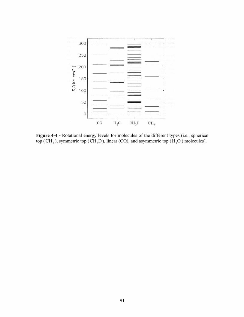
Finally, possible rotational energy levels for molecules of the different types (i.e., spherical top, symmetrical top, linear, and asymmetric top molecules) are shown in Figure 4-4.

91

Figure 4-4 - Rotational energy levels for molecules of the different types (i.e., spherical top (CH4 ), symmetric top (CH3D ), linear (CO), and asymmetric top (H2O ) molecules).