Embed Size (px)
Citation preview

Chapter 4
The quantum theory of light
In this chapter we study the quantum theory of interaction between light and mat-ter. Historically the understanding how light is created and absorbed by atomswas central for development of quantum theory, starting with Planck’s revolution-ary idea of energy quanta in the description of black body radiation. Even if nowthe theoretical understanding of the quantum theory of light is embedded withinthe more complete quantum field theory with applications to the physics of el-ementary particles, the quantum theory of light and atoms has continued to beimportant and to be developed further. We will study the quantum description ofthe free electromagnetic field and the description of single photon processes. Butwe will also examine some coherent many-photon processes that are important inthe application of quantum optics today.
4.1 Classical electromagnetism
The Maxwell theory of electromagnetism is the basis for the classical as wellas the quantum description of radiation. With some modifications due to gaugeinvariance and to the fact that this is a field theory (with an infinite number ofdegrees of freedom) the quantum theory can be derived from classical theory bythe standard route of canonical quantization. In this approach the natural choiceof generalized coordinates correspond to the field amplitudes.
In this section we make a summary of the classical theory and show how a La-grangian and Hamiltonian formulation of electromagnetic fields interacting withpoint charges can be given. At the next step this forms the basis for the quantumdescription of interacting fields and charges.
105
106 CHAPTER 4. THE QUANTUM THEORY OF LIGHT
4.1.1 Maxwell’s equations
Maxwell’s equations (in Heaviside-Lorentz units) are
∇ · E = ρ
∇ × B − 1
c
∂E
∂t=
1
cj
∇ · B = 0
∇ × E +1
c
∂B
∂t= 0 (4.1)
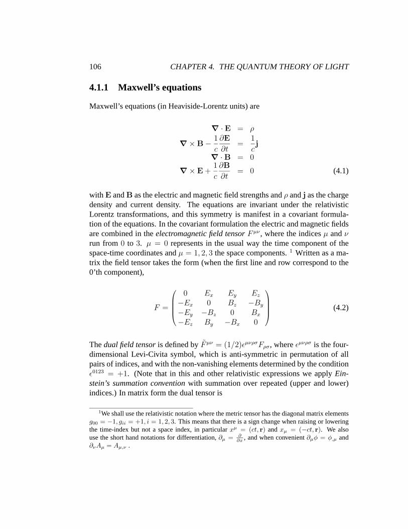
with E and B as the electric and magnetic field strengths and ρ and j as the chargedensity and current density. The equations are invariant under the relativisticLorentz transformations, and this symmetry is manifest in a covariant formula-tion of the equations. In the covariant formulation the electric and magnetic fieldsare combined in the electromagnetic field tensor F µν , where the indices µ and νrun from 0 to 3. µ = 0 represents in the usual way the time component of thespace-time coordinates and µ = 1, 2, 3 the space components. 1 Written as a ma-trix the field tensor takes the form (when the first line and row correspond to the0’th component),
F =
0 Ex Ey Ez
−Ex 0 Bz −By
−Ey −Bz 0 Bx
−Ez By −Bx 0
(4.2)
The dual field tensor is defined by F µν = (1/2)εµνρσFρσ, where εµνρσ is the four-dimensional Levi-Civita symbol, which is anti-symmetric in permutation of allpairs of indices, and with the non-vanishing elements determined by the conditionε0123 = +1. (Note that in this and other relativistic expressions we apply Ein-stein’s summation convention with summation over repeated (upper and lower)indices.) In matrix form the dual tensor is
1We shall use the relativistic notation where the metric tensor has the diagonal matrix elementsg00 = −1, gii = +1, i = 1, 2, 3. This means that there is a sign change when raising or loweringthe time-index but not a space index, in particular xµ = (ct, r) and xµ = (−ct, r). We alsouse the short hand notations for differentiation, ∂µ = ∂
∂x , and when convenient ∂µφ = φ,µ and∂νAµ = Aµ,ν .

4.1. CLASSICAL ELECTROMAGNETISM 107
F =
0 Bx By Bz
−Bx 0 −Ez Ey
−By Ez 0 −Ex
−Bz −Ey Ex 0
(4.3)
When written in terms of the field tensors and the and the 4-vector current densityjµ = (c ρ, j) Maxwell’s equations gets the following compact form
∂νFµν =
1
cjµ
∂νFµν = 0 (4.4)
The Maxwell equations are, except for the presence of source terms, sym-metric under the duality transformation F µν → F µν , which corresponds to thefollowing interchange of electric and magnetic fields
E → B , B → −E (4.5)
In fact, the equations for the free fields are invariant under a continuous electric-magnetic transformation, which is an extension of the discrete duality transfor-mation,
E → cos θE + sin θB
B → − sin θE + cos θB (4.6)
This symmetry is broken by the source terms of the Maxwell equation.Formally the symmetry can be restored by introducing magnetic charge and
magnetic current in addition to electric charge and current. In such an extendedtheory there would be two kinds of sources for electromagnetic fields, electriccharge and magnetic charge, and in the classical theory such an extension wouldbe unproblematic. However for the corresponding quantum theory, some interest-ing complications would arise. The standard theory is based on the use of elec-tromagnetic potentials, which depend on the “magnetic equations” being sourcefree.
A consistent quantum theory can however be formulated with magnetic charges,provided both electric and magnetic charges are associated with point particles and
108 CHAPTER 4. THE QUANTUM THEORY OF LIGHT
provided they satisfy a quantization condition.2 This is interesting, since such aconsistence requirement would give a fundamental explanation for the observedquantization of electric charge. Theoretical considerations like this have, over theyears, lead to extensive searches for magnetic charges (or magnetic monopoles),but at this stage there is no evidence for the existence of magnetic charges innature.
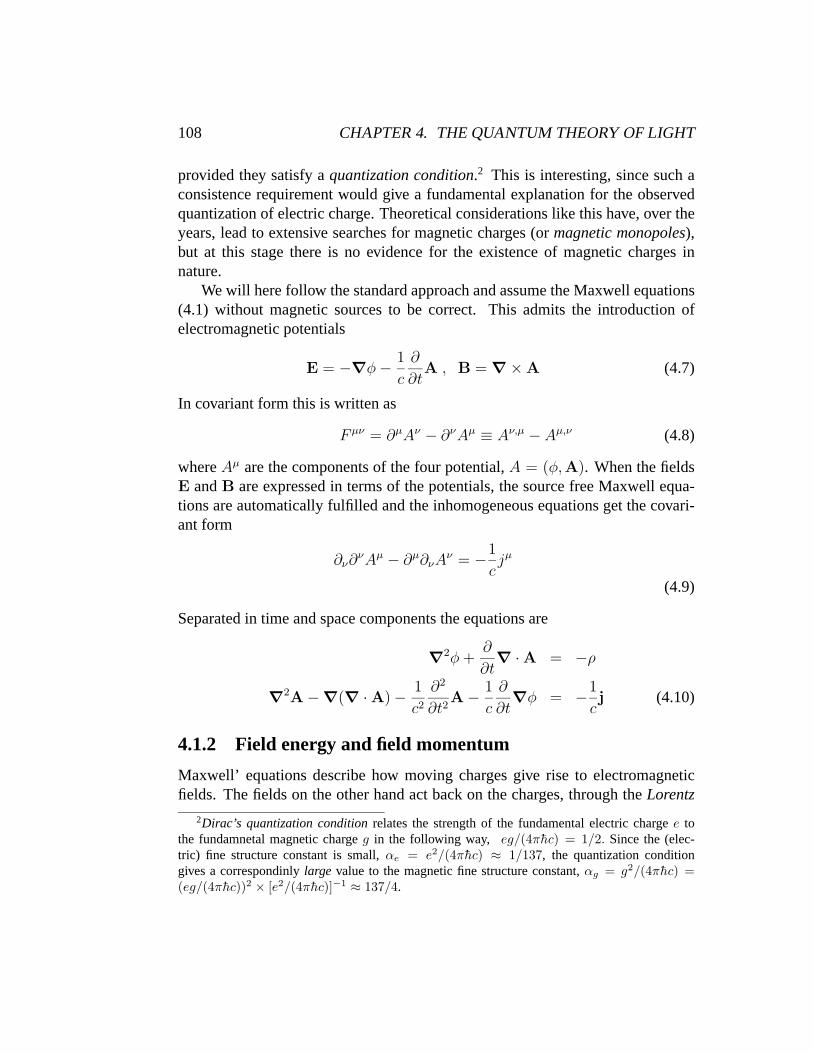
We will here follow the standard approach and assume the Maxwell equations(4.1) without magnetic sources to be correct. This admits the introduction ofelectromagnetic potentials
E = −∇φ − 1
c
∂
∂tA , B = ∇ × A (4.7)
In covariant form this is written as
F µν = ∂µAν − ∂νAµ ≡ Aν,µ − Aµ,ν (4.8)
where Aµ are the components of the four potential, A = (φ,A). When the fieldsE and B are expressed in terms of the potentials, the source free Maxwell equa-tions are automatically fulfilled and the inhomogeneous equations get the covari-ant form
∂ν∂νAµ − ∂µ∂νA
ν = −1
cjµ
(4.9)
Separated in time and space components the equations are
∇2φ +∂
∂t∇ · A = −ρ
∇2A − ∇(∇ · A) − 1
c2
∂2
∂t2A − 1
c
∂
∂t∇φ = −1
cj (4.10)
4.1.2 Field energy and field momentum
Maxwell’ equations describe how moving charges give rise to electromagneticfields. The fields on the other hand act back on the charges, through the Lorentz
2Dirac’s quantization condition relates the strength of the fundamental electric charge e tothe fundamnetal magnetic charge g in the following way, eg/(4πhc) = 1/2. Since the (elec-tric) fine structure constant is small, αe = e2/(4πhc) ≈ 1/137, the quantization conditiongives a correspondinly large value to the magnetic fine structure constant, αg = g2/(4πhc) =(eg/(4πhc))2 × [e2/(4πhc)]−1 ≈ 137/4.

4.1. CLASSICAL ELECTROMAGNETISM 109
force, which for a pointlike charge q it has the form
F = q(E +v
c× B) (4.11)
When the field is acting with a force on the charged particles this implies thatenergy and momentum is transferred between the field and the particles. Thus, theelectromagnetic field carries energy and momentum, and the form of the energyand momentum density can be determined from Maxwell’s equation and the formof the Lorentz force, by assuming conservation of energy and conservation ofmomentum.
To demonstrate this we consider a single pointlike particle is affected by thefield, and the charge and momentum density therefore can be expressed as
ρ(r, t) = q δ(r − r(t))
j(r, t) = q v(t) δ(r − r(t)) (4.12)
where r(t) and v(t) describe the posision and velocity of the particle of the particleas functions of time. The time derivative of the field energy E will equal the effectof the work performed on the particle
d
dtE = −F · v = −qv · E (4.13)
By use of the field equations we re-write it in the following way
d
dtE = −
∫d3r j · E
= −∫
d3r[cE · (∇ × B) − E · ∂E
∂t
]
=∫
d3r[E · ∂E
∂t+ B · ∂B
∂t− c∇ · (E × B)
]
=d
dt
1
2
∫d3r
[E2 + B2
](4.14)
where in the last step surface terms in the integral have been disregarded, since wemay assume that the fields fall off sufficiently rapid at infinity. The correspondingexpression for the energy is
E =∫
d3r1
2
[E2 + B2
](4.15)
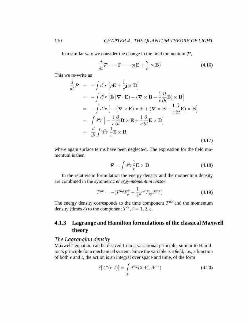
110 CHAPTER 4. THE QUANTUM THEORY OF LIGHT
In a similar way we consider the change in the field momentum P ,
d
dtP = −F = −q(E +
v
c× B) (4.16)
This we re-write as
d
dtP = −
∫d3r
[ρE +
1
cj × B
]
= −∫
d3r[E (∇ · E) + (∇ × B − 1
c
∂
∂tE) × B
]
= −∫
d3r[− (∇ × E) × E + (∇ × B − 1
c
∂
∂tE) × B
]
=∫
d3r[− 1
c
∂
∂tB × E +
1
c
∂
∂tE × B
]
=d
dt
∫d3r
1
cE × B
(4.17)
where again surface terms have been neglected. The expression for the field mo-mentum is then
P =∫
d3r1
cE × B (4.18)
In the relativistic formulation the energy density and the momentum densityare combined in the symmetric energy-momentum tensor,
T µν = −(F µρF νρ +
1
4gµνFρσF ρσ) (4.19)
The energy density corresponds to the time component T 00 and the momentumdensity (times c) to the component T 0i, i = 1, 2, 3.
4.1.3 Lagrange and Hamilton formulations of the classical Maxwelltheory
The Lagrangian densityMaxwell’ equation can be derived from a variational principle, similar to Hamil-ton’s principle for a mechanical system. Since the variable is a field, i.e., a functionof both r and t, the action is an integral over space and time, of the form
S[Aµ(r, t)] =∫
Ω
d4xL(Aµ, Aµ,ν) (4.20)
4.1. CLASSICAL ELECTROMAGNETISM 111
where L is the Lagrangian density and Ω is the chosen space-time region. TheLagrangian density is a local function of the field variable Aµ and its derivative,
L = −1
4FµνF
µν +1
cAµjµ (4.21)
with F µν = Aν,µ − Aµ,ν treated as a derivative of the field variable.A dynamical field, i.e., a solution of Maxwell’s equations for given boundary
conditions (on the boundary of Ω), corresponds to a solution of the variationalequation,
δS = 0 (4.22)
where this condition should be fulfilled for arbitrary variations in the field vari-ables, with fixed values on the boundary of Ω. The equivalence between this vari-ational equation and the differential (Maxwell) equations is shown in the sameway as for the equation of motion of a mechnical system, with a discrete set ofcoordinates.
The variation in S is, to first order in the variation of the field variable Aµ,given by
δS =∫
Ω
d4x[ ∂L∂Aµ
− ∂ν
( ∂L∂Aµ,ν
)]δAµ (4.23)
where in this expression we have made a partial integration and used the factthat δAµ vanishes on the boundary of Ω. Since the variation should otherwisebe free, the variational equation (4.22) is satisfied only if the field satisfies theEuler-Lagrange equation
∂L∂Aµ
− ∂ν
( ∂L∂Aµ,ν
)= 0 (4.24)
With L given by (4.21) it is straight forward to check that the Euler-Lagrangeequation reproduces the inhomogeneous Maxwell equations.
The canonical field momentumThe Lagrange and Hamilton formulations give equivalent descriptions of the dy-namics in analytical mechanics. Also in the case of field theories, a Hamiltoniancan be derived from the Lagrangian density, but with electromagnetism there aresome complications to be dealt with. We first note that the Lagrangian formu-lation is well suited to fit the relativistic invariance of the theory, since it makes

112 CHAPTER 4. THE QUANTUM THEORY OF LIGHT
no difference in the treatment of the space and time coordinates. That is not sofor the Hamiltonian formulation, which does distinguish the time direction. Thiscarries over to the (standard) quantum description, where time is distinguished inthe Schrodinger equation. This does not mean that relativistic invariance cannotbe incorporated in the Hamiltonian description, but it is not as explicit as in theLagrange formulation.
To define the Hamiltonian we first need to identify a set of independent vari-ables and their corresponding canonical momenta. As field variables we tenta-tively use the potential Aµ(r), where r can be viewed as a continuous and µ as adiscrete index for the field coordinate. (For a mechanical system r and µ corre-spond to the discrete index k which labels the independent generalized coordinatesqk.) Like the field variable, the canonical momentum now is a field, πµ = πµ(r).It is defined by
πµ =∂L∂Aµ
=1
c
∂L∂Aµ,0
(4.25)
We note here the different treatment of the time and space coordinate.The Lagrangian density (4.21) gives the following expression for the canonical
field momentum
πµ =1
c
∂
∂Aµ,0
[− 1
2(Aµ,νA
µ,ν − Aµ,νAν,µ) − 1
cAµjµ
]
=1
cF µ0 (4.26)
The space part (µ = 1, 2, 3) is proportional to the electric field, but note thatthe time component vanishes, π0 = 0. Also note that the canonical momen-tum defined by the Lagrangian is this way is not directly related to the physicalmomentum carried by the electromagnetic field, as earlier has been found frommomentum conservation.
The fact that there is no canonical momentum corresponding to the field com-ponent A0 indicates that the choice we have made for the generalized coordinatesof the electromagnetic field is not complitely satisfactory. The field amplitudesAµ cannot all be seen as describing independent degrees of freedom. This has todo with the gauge invariance of the theory, and we proceed to discuss how thisproblem can be handled.
Gauge invariance and gauge fixing

4.1. CLASSICAL ELECTROMAGNETISM 113
We consider the following transformation of the electromagnetic potentials
A → A′ = A + ∇χ , φ → φ′ = φ +1
c
∂
∂tχ (4.27)
where χ is a (scalar) function of space and time. In covariant form it is
Aµ → Aµ′ = Aµ + ∂µχ (4.28)
This is a gauge transformation of the potentials, and it is straight forward to showthat such a transformation leaves the field strengths E and B invariant. The usualway to view the invariance of the fields under this transformation is that it reflectsthe presence of a non-physical degree of freedom in the potentials. The poten-tials define an overcomplete set of variables for the electromagnetic field. Forthe Hamiltonian formulation to work it is necessary to identify the independent,physical degrees of freedom.
There are two different constraints, or gauge conditions, that are often used toremove the unphysical degree of freedom associated with gauge invariance. TheCoulomb (or radiation) gauge condition is
∇ · A = 0 (4.29)
and the Lorentz (or covariant) gauge condition is
∂µAµ = 0 (4.30)
The first one is often used when the interaction between radiation and atoms isconsidered, since the electrons then move non-relativistically and therefore thereis no need for a covariant form of the gauge condition. This is the condition wewill use here. The Lorentz gauge condition is often used in the description of in-teraction between radiation and relativistic electrons and other charged particles.The relativistic form of the field equations then are not explicitely broken by thegauge condition, but the prize to pay is that in the quantum description one has toinclude unphysical photon states.
Hamiltonian in the Coulomb gaugeIn Coulomb gauge Maxwell’s (inhomogeneous) equations reduce to the followingform
∇2φ = −ρ (4.31)
(1
c2
∂2
∂t2− ∇2)A =
1
cjT (4.32)

114 CHAPTER 4. THE QUANTUM THEORY OF LIGHT
Where
jT = j − ∂
∂t∇φ (4.33)
is the transverse component of th current density.3 It satisfies the transversalitycondition as a consequence of the continuity equation for charge,
∇ · jT = ∇ · j − ∂
∂t∇2φ
= ∇ · j +∂
∂tρ
= 0 (4.34)
We note that the equation for the scalar field φ contains no time derivatives, andcan be solved in tems of the charge distribution,
φ(r, t) =∫
d3r′ρ(r′, t)
4π|r − r′| (4.35)
This is the electrostatic (Coulomb) potential of a stationary charge distributionwhich coincides with the true charge distribution ρ(r, t) at time t. Note that the rel-ativistic retardation effects associated with the motion of charges are not present,and the vector potential A is therefore needed to give the correct relativistic formof the electromagnetic field set up by the charges.
The φ-field carries no independent degrees of freedom of the electromagneticfield, it is fully determined by the position of the charges. The dynamics of theMaxwell field is then carried solely by the vector potential A. In the quantumdescription the photons are therefore associated only with the field amplitude Aand not with φ.4
3Any vector field j(r) can be written as j = jT + jL, where ∇ · jT = 0 and ∇×jL = 0. jT isreferred to as the transverse or solenoidal part of the field and jL as the longitudinal or irrotationalpart of the field. In the present case, with jL = −∇φ the irrotational form of jL follows directly,while the transversality of jT follows from charge conservation.
4A curious consequence is that whereas for a stationary charge there are no photons present,only the non-dynamical Coulomb field, for a uniformly moving charge there will be a ”cloud” ofphotons present to give the field the right Lorentz transformed form. This is so even if there isno radiation from the charge. We may see this as a consequence of the Coulomb gauge conditionand our separation of the system into field degrees of freedom (photons) and particle degrees offreedom. In reality, for the interacting system of charges and fields this separation is not so clear,since on one hand the Coulomb field is non-dynamically coupled to the charges, and on the otherhand is dynamically coupled to the radiation field.

4.1. CLASSICAL ELECTROMAGNETISM 115
Expressed in terms of the dynamical A field the Lagrangian density gets theform
L = −1
4FµνF
µν +1
cjµA
µ
=1
2c2A2 +
1
cA · ∇φ +
1
2(∇φ)2 − 1
2(∇ × A)2 +
1
cj · A − ρφ(4.36)
Two of the terms we re-write as
1
cA · ∇φ =
1
c∇ · (Aφ) − 1
cφ∇ · A
=1
c∇ · (Aφ) (4.37)
and
1
2(∇φ)2 =
1
2∇ · (φ∇φ) − 1
2(φ∇2φ)
=1
2∇ · (φ∇φ) +
1
2ρφ (4.38)
where the Coulomb gauge condition has been used in the first equation. We notethat the divergences in these expressions give unessential contributions to the La-grangian and can be deleted. This is so since divergences only give rise to surfaceterms in the action integral and therefore do not affect the field equations.
With the divergence terms neglected the Lagrangian density gets the form 5
L =1
2c2A2 − 1
2(∇ × A)2 +
1
cj · A − 1
2ρφ (4.39)
The field degrees of freedom are now carried by the components of the vectorfield, which still has to satisfy the constraint equation ∇ · A = 0. The conjugatemomentum is
π =1
c2· A ≡ −1
cET (4.40)
5In this expression we have used the freedom to replace the transverse current jT with the fullcurrent j, which is possible since the difference gives rise to an irrelevant derivative term. Note,however, that when the full current is used, the transversality condition ∇ ·A has to be imposed asa constraint to derive the correct field equations from the Lagrangian. When the A-field is coupledto the transverse current, that is not needed.

116 CHAPTER 4. THE QUANTUM THEORY OF LIGHT
where ET denotes the transverse part of the electric field, the part where −∇φ isnot included.
So far we have not worried about the degrees of freedom associated with thecharges. We will now include them in the description by assuming the charges tobe carried by point particles. This means that we express the charge density andcurrent as
ρ(r, t) =∑
i
eiδ(r − ri(t))
j(r, t) =∑
i
eivi(t)δ(r − ri(t)) (4.41)
where the sum is over all the particles with ri(t) and vi(t) as the position andvelocity of particle i as functions of time. The action integral of the full interactingsystem we write as
S =∫
d3rL =∫
d3r(Lfield + Lint + Lpart) (4.42)
where Lfield + Lint is the space integral of the Lagrangian density (4.39) andLpart is the standard Lagrangian of free non-relativisic particles. By performingthe space integral over the charge density and current, we find the following ex-pression for the Lagrangian,6
L =∫
d3r[ 1
2c2A2 − 1
2(∇ × A)
]+
∑i
ei
cvi · A(ri)
−1
2
∑i=j
eiej
4π[ri − rj|+
∑i
1
2miv
2i (4.43)
The corresponding Hamiltonian is found by performing a (Legendre) transforma-tion of the Lagrangian in the standard way
H =∫
d3r π · A +∑
i
pi · vi − L
=∫
d3r (E2T + B2) +
∑i<j
eiej
4π[ri − rj|+
∑i
1
2mi
(p − ei
cA(ri))
2
(4.44)6For point charges an ill-defined self energy contribution may seem to appear from the
Coulomb interaction term. It is here viewed as irrelevant since it gives no contribution to theinteraction between the particles and is therefore not included. In a more complete field theo-retic treatment of the interaction of charges and fields such problems will reappear and have to behandled within the framework of renormalization theory.

4.2. PHOTONS – THE QUANTA OF LIGHT 117
This expression for the Hamiltonian is derived for the classical system of inter-acting fields and particles, but it has the same form as the Hamiltonian operatorthat is used to describe the quantum system of non-relativistic electrons interact-ing with the electromagnetic field. However, to include correctly the effect of themagnetic dipole moment of the electrons, a spin contribution has to be added tothe Hamiltonian. It has the standard form of a magnetic dipole term,
Hspin = −∑
i
giei
2micSi · B(ri) (4.45)
where gi is the g-factor of particle i, which is close to 2 for electrons. Oftenthe spin term is small corresponding to the other interaction terms and can beneglected.
4.2 Photons – the quanta of light
With the degrees of freedom of the electromagnetic field and of the electronsdisentangled, we may consider the space of states of the full quantum system asthe product space of a field-state space and a particle-state space,
H = Hfield ⊗Hparticle (4.46)
In this section we focus on the quantum description of the free electromagneticfield, which defines the space Hfield and the operators (observables) acting there.The energy eigen states of the free field are the photon states. When we as anext step include interactions, these will introduce processes where photons areemitted and absorbed.
4.2.1 Constructing Fock space
Since the field amplitude A is constrained by the transversality condition ∇ ·A = 0 it is convenient to make a Fourier transform to plane wave amplitudes.In a standard way we introduce a periodicity condition on the components of thespace coordinate r, so that the Fourier variable ki = 2πni/L with L as a (large)periodic length and ni as a set of integers for the components i = 1, 2, 3. The fieldamplitude then can be written as a discrete Fourier sum
A(r, t) =1√V
∑k
2∑a=1
Aka(t)εkaeik·r (4.47)

118 CHAPTER 4. THE QUANTUM THEORY OF LIGHT
where the V = L3 is the normalization volume and the vectors εka are unit vectorswhich satisfy the transversality condition k·εka = 0. There is no further constrainton the transverse amplitudes Aka, which can be taken to represent the independentdegrees of freedom of the field.
We note that the corresponding solutions of the classical field equations arethe normal modes of the field, which in free space are the plane wave solutions,
Aka(t) = A0kae
±iωkt , ωk = ck (k = |k|) (4.48)
They represent waves of monochromatic, polarized light. The two vectors εka arethe polarization vectors, which may be taken to be two orthonormal, real vectorsperpendicular to k. The two field modes then correspond to linearly polarizedplane waves. The polarization vectors may also be taken as complex superposi-tions of the two real vectors, in which case they correspond to circularly, or moregenerally to elliptically polarized light.
The Lagrangian of the free electromagnetic field expressed in terms of theFourier amplitudes is
L =1
2
∑ka
[ 1
c2A∗
kaAka − k2A∗kaAka
](4.49)
We note that there is no coupling between the different Fourier components, andfor each component the Lagrangian has the same form as for a harmonic oscil-lator of frequency ω = ck. The variables are however complex rather than real,since reality of the field A(r) gives a relation between Fourier components withdifferent values of k,
A∗ka = A−ka (4.50)
where a is defined by εka = ε−ka. Thus, the variables in (4.49) correspond tothe complex coordinate z of the harmonic oscillator rather than the real x. Arewriting of the Lagrangian in tems of real variables is straight forward, but it ismore convenient to continue to work with the complex variables.
The conjugate momentum to the variable Aka is
Πka =1
c2A∗
ka = −1
cE∗
ka (4.51)
where Eka is the Fourier component of the electric field. From this the form ofthe free field Hamiltonian is found
H =∑ka
ΠkaAka − L

4.2. PHOTONS – THE QUANTA OF LIGHT 119
=∑ka
1
2(E∗
kaEka + k2A∗kaAka) (4.52)
which is consistent with the earlier expression found for the Hamiltonian of theelectromagnetic field (4.44).
Quantization of the theory means that the classical field amplitude and fieldstrength are now replaced by operators, which satisfy the canonical commutationrelations
[E†
ka, Ak′b
]= −1
c
[˙A
†ka, Ak′b
]= −ihc δkk′ δab (4.53)
It is convenient to change to new variables,
Aka = c
√h
2ωk
(aka + a†−ka)
Eka = i
√h
2ωk
(aka − a†−ka) (4.54)
where the reality condition (4.50) has been made explicit. In tems of the newvariables the Hamiltonian takes the form
H =∑ka
1
2hωk(akaa
†ka + a†
kaaka) (4.55)
and the canonical commutation relations are[aka, a
†k′b
]= δkk′δab
[aka, ak′b] = 0 (4.56)
Expressed in this way the Hamiltonian has exactly the form of a collection ofindependent quantum oscillator, one for each field mode, with aka as lowering op-erator and a†
ka as raising operator in the energy spectrum of the oscillator labelledby (ka).
It is convenient to work, in the following, in the Heisenberg picture, where theobservables are time dependent. In this picture the field amplitude, which is nowa field operator, and the electric field get the following form,
A(r, t) =∑ka
c
√h
2V ωk
[akaεkae
i(k·r−ωkt) + a†kaε
∗kae
−i(k·r−ωkt)]
E(r, t) = i∑ka
√hωk
2V
[akaεkae
i(k·r−ωkt) − a†kaε
∗kae
−i(k·r−ωkt)]
(4.57)

120 CHAPTER 4. THE QUANTUM THEORY OF LIGHT
The state space of the free electromagnetic field then can be viewed as a prod-uct space of harmonic oscillator spaces, one for each normal mode of the field.The vacuum state is defined as the ground state of the Hamiltonian (4.55), whichmeans that it is the state where all oscillators are unexcited,
aka|0〉 = 0 (4.58)
The operator a†ka, which excites one of the oscillators, is interpreted as a creation
operator which creates one photon from the vacuum,
a†ka|0〉 = |1ka〉 (4.59)
An arbitrary number of photons can be created in the same state (ka),
(a†ka)
n|0〉 =√
nka! |nka〉 (4.60)
and this shows that the photons are bosons. The operator aka is an annihilationoperator which reduces the number of photons in the state ka,
aka|nka〉 =√
nka |nka − 1〉(4.61)
The photon number operator is
Nka = a†kaaka (4.62)
It counts the number of photons present in the state (ka),
Nka|nka〉 = nka |nka〉 (4.63)
The general photon state, often referred to as a Fock state, is a product statewith a well-defined number of photons for each set of quantum nubers (ka). It isspecified by a set of occupation numbers nka for the single-photon states. Theset of Fock states |nka〉 form a basis of orthonormal states that span the statespace, the Fock space, of the quantized field. Thus a general quantum state of thefree electromagnetic field is a linear superposition of Fock states,
|ψ〉 =∑
nkac(nka)|nka〉 (4.64)

4.2. PHOTONS – THE QUANTA OF LIGHT 121
The energy operator, which is identical to the Hamiltonian, has the same formas the classical field energy. It is diagonal in the Fock basis and can be expressedin terms of the photon number operator
H =∫
d3r1
2(E2 + B2)
=∑ka
1
2hωk(a
†kaaka + akaa
†ka)
=∑ka
hωk(Nka +1
2) (4.65)
One should note that the vacuum energy is formally infinite, since the sum over theground state energy 1
2ωk for all the oscillators diverges. However, since this is an
additive constant which is common for all states it can be regarded as unphysicaland simply be subtracted. The vacuum energy is on the other hand related tovacuum fluctuations and in this way it is connected to properties of the quantumtheory that has real, physical effects.
In a similar way the classical field momentum is replaced by an operator ofthe same form,
P =∫
d3r1
c(E × B)
=∑ka
1
2hk(a†
kaaka + akaa†ka)
=∑ka
hkNka (4.66)
The energy-momentum relation for a single photon, hωk = h|k|, shows that thephotons behave like massless particles.
4.2.2 Coherent and incoherent photon states
In the same way as for the quantum description of single particles, we may viewexpectation values of the fields to represent classical field configurations withinthe quantum description. The fields will not be sharply defined since there willin general be quantum fluctuations around the expectation values. In particularwe note that the expectation value of the electric field takes the usual form of aclassical field expanded in plane wave components
⟨E(r, t)
⟩= i
∑ka
√hωk
2V
[αkaεkae
i(k·r−ωkt) − α∗kaε
∗kae
−i(k·r−ωkt)]
(4.67)
122 CHAPTER 4. THE QUANTUM THEORY OF LIGHT
where αka and α∗ka are expectation values of the annihilation and creation opera-
tors.
αka = 〈aka〉 , α∗ka =
⟨a†ka
⟩(4.68)
We note from these expressions the curious fact that for Fock states, with asharply defined set of photon numbers, the expectation values vanish. Such stateswhich may be highly excited in energy, but still with vanishing expectation valuesfor electric and magnetic fields are highly non-classical states. Classical fields, onthe other hand, correspond to states with a high degree of coherence, in the form ofsuperposition between Fock states. As already discussed for the one-dimensionalharmonic oscillator, the coherent states are minimum uncertainty states in thephase spase variables. Here these variables are represented by the field amplitudeA(r, t) and the electric field strength E(r, t). For a single field mode the coherentstate has the form as discussed in section (1.3.3) for the harmonic oscillator
|αka〉 =∑nka
e−12|αka|2 (αka)
nka
√nka!
|nka〉 (4.69)
where αka is related to the expectation values of aka and a†ka as in (4.68). The full
coherent state of the electromagnetic field is then a product state of the form
|ψ〉 =∏ka
|αka〉 (4.70)
and the expectation value of the electric field is given by (4.67).The fluctuations in the electric field for the coherent state can be evaluated in
terms of the following correlation function
Cij(r − r′) ≡ 〈Ei(r)Ej(r′)〉 − 〈Ei(r)〉 〈Ej(r
′)〉
=∑ka
hωk
2Veik·(r−r′)(δij −
kikj
k2)
→ ch
2(2π)3
∫d3kkeik·(r−r′)(δij −
kikj
k2) (4.71)
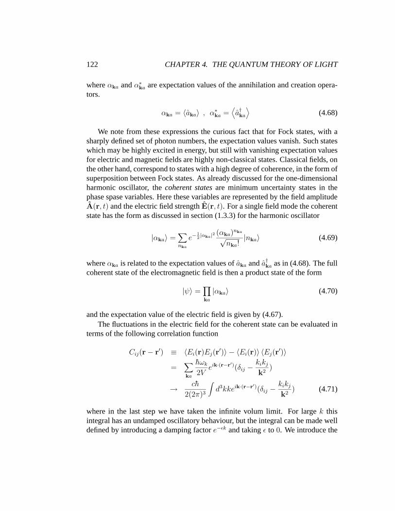
where in the last step we have taken the infinite volum limit. For large k thisintegral has an undamped oscillatory behaviour, but the integral can be made welldefined by introducing a damping factor e−εk and taking ε to 0. We introduce the
4.2. PHOTONS – THE QUANTA OF LIGHT 123
1.5 2 2.5 3 3.5 4
0.2
0.4
0.6
0.8
1
C
|r-r'|
Figure 4.1: The correlation function for the electric field in a coherent state,Cij(r − r′) ≡ 〈Ei(r)Ej(r
′)〉 − 〈Ei(r)〉 〈Ej(r′)〉. The form of the non-vanishing
elements, i = j, is shown as the function of distance r− r′ between two points inspace.
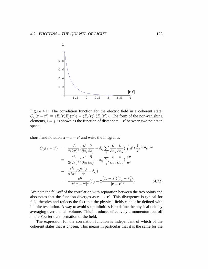
short hand notation a = r − r′ and write the integral as
Cij(r − r′) =ch
2(2π)3(
∂
∂ai
∂
∂aj
− δij
∑k
∂
∂ak
∂
∂ak
)∫
d3k1
keik·ae−εk
=ch
2(2π)3(
∂
∂ai
∂
∂aj
− δij
∑k
∂
∂ak
∂
∂ak
)4π
a2
=ch
π2a4(2
aiaj
a2− δij)
= − ch
π2|r − r′|4 (δij − 2(xi − x′
i)(xj − x′j)
|r − r′|2 ) (4.72)
We note the fall-off of the correlation with separation between the two points andalso notes that the function diverges as r → r′. This divergence is typical forfield theories and reflects the fact that the physical fields cannot be defined withinfinite resolution. A way to avoid such infinities is to define the physical field byaveraging over a small volume. This introduces effectively a momentum cut-offin the Fourier transformation of the field.
The expression for the correlation function is independent of which of thecoherent states that is chosen. This means in particular that it is the same for the

124 CHAPTER 4. THE QUANTUM THEORY OF LIGHT
vacuum state and can be viewed as demonstrating the presence of the vacuumfluctuations of the electric field.
A similar calculation for the magnetic field shows that the correlation functionis the same as for the electric field. This is typical for the coherent state whichis symmetric in its dependence of the field variable and its conjugate momentum.Since A and E are conjugate variables, the electric and magnetic fields do notcommute as operator fields. Formally the commutator is
[Bi(r), Ej(r′)] = δij∇ × δ(r − r′) (4.73)
where one should express it in terms of the Fourier transformed fields in orderto give it a more precise meaning. There are states where the fluctuations in theE-field are supressed relative to that of the vacuum state, but due to the non-vanishing of the commutator with B, the fluctuations in the B-field will then belarger than that of the vacuum. States with reduced fluctuations in one of thefields, and which still satisfy the condition of minimum (Heisenberg) uncertaintyfor conjugate variables, are often referred to as squeezed states.
Radio waves, produced by oscillating currents in an antenna, can clearly beregarded as classical electromagnetic waves and are well described as coherentstates of the electromagnetic field within the quantum theory of radiation. Themean value of the fields at the receiver antenna induces the secondary currentthat creates the electric signal to the receiver. Also for shorter wavelengths in themicrowave and the optical regimes coherent states of the electromagnetic can becreated, but not by oscillating macroscopic currents. In masers and lasers the in-trinsic tendency of atoms to correlate their behaviour in a strong electromagneticfield is used to create a monocromatic beam with a high degree of coherence.Ordinary light, on the other hand, as emitted by a hot source is highly incoher-ent, since the emission from different atoms only to a low degree is correlated.This means that normal light is highly non-classical in the sense that it cannot beassociated with a classical wave with oscillating (macroscopic) values of E andB.
To demonstrate explicitely the non-classical form on the radiation from a hotsource, we consider light in a thermal state described by a density operator of theform
ρ = N e−βH , N = (Tr e−βH)−1 , β = (kBT )−1
(4.74)
We first calculate the expectation value of the photon numbers
nka ≡⟨Nka
⟩

4.2. PHOTONS – THE QUANTA OF LIGHT 125
= N Tr (e−βhωa†ka
aka a†kaaka)
= N Tr(e−βhωa†ka
aka a†kae
βhωa†ka
aka e−βhωa†ka
aka aka)
= N Tr(e−βhω a†ka e−βhωa†
kaaka aka)
= e−βhωN Tr( e−βhωa†ka
aka akaa†ka)
= e−βhωN Tr(e−βhωa†ka
aka(a†kaaka + 1))
= e−βhω(nka + 1) (4.75)
which gives
nka =1
eβhω − 1(4.76)
This is the well-known Bose-Einstein distribution for photons in thermal equilib-rium with a heat bath. From this distribution the Planck spectrum can be deter-mined. The total radiation energy is
E =∑ka
hωknka
→ 2V
(2π)3
∫d3k
hωk
eβhωk − 1
=V h
π2c3
∫dω
ω3
eβhω − 1(4.77)
This corresponds to the following energy density per frequency unit to be
u(ω) =h
π2c3
ω3
eβhω − 1(4.78)
which displays the form of the Planck spectrum.We now consider the expectation values of the photon annihilation and cre-
ation operators. A similar calculation as for the number operator gives⟨a†ka
⟩= N Tr(e−βhωa†
kaaka a†
ka)
= N Tr(e−βhωa†ka
aka a†kae
βhωa†ka
aka e−βhωa†ka
aka)
= N Tr(e−βhω a†ka e−βhωa†
kaaka)
= e−βhωN Tr( e−βhωa†ka
aka a†ka)
= e−βhω⟨a†ka
⟩(4.79)

126 CHAPTER 4. THE QUANTUM THEORY OF LIGHT
radiation
2000 K
1500 K
1000 K
wave length [nm]
2000 4000 6000heat bath
cavity
detector inte
nsi
ty
Figure 4.2: The Planck spectrum. A schematic experimental set up is shownwhere thermal light is created in a cavity surrounded by a heat bath (an oven).The radiation escapes through a narrow hole and can be analyzed in a detector.The right part of the figure shows the intensity (energy density) of the radiation asa function of wave length for three different temperatures.
This shows that the expectation value of the creation operator vanishes. A similarreasoning applies to the annihilation operator, so that
⟨a†ka
⟩= 〈aka〉 = 0 (4.80)
As a consequence the expectation value of the electric and magnetic field vanishidentically
〈E(r, t)〉 = 〈B(r, t)〉 = 0 (4.81)
The last result for the expectation values of the electric and magnetic fieldstrengths may be expected since thermal ligth is unpolarized. Due to rotationalinvariance no direction can be distinguished, which means that the expectationvalues for the vector fields E and B should vanish. We note that in a classical de-scription the E and B fields cannot vanish identically unless there is no radiationpresent. Rotational invariance can therefore be restored for a classical radiationfield only by introducing statistical fluctuatuations in the fields which averageout the field without setting E2 and B2 to zero. However, the form of the den-sity matrix (4.74) shows that the vanishing of the expectation values is not dueto statistical averaging over classical configurations. The density matrix can be

4.2. PHOTONS – THE QUANTA OF LIGHT 127
interpreted as describing an incoherent mixture (i.e., a statistical ensemble) of en-ergy eigenstates, where each of these is a Fock state with vanishing expectationvalues for the electromagnetic field strengths. The vanishing of the expectationvalues therefore is due to quantum fluctuations of the fields rather than statisticalfluctuations.
This view of light, that it cannot be seen as (a statitistical mixture of), classicalfield configurations may seem to be problematic when confronted with the classi-cal demonstrations of the wave nature of light, in particular Young’s interferenceexperiments. This experiment seems to confirm the picture of light as (classical)waves that can interfere constructively or destructvely, depending on the relativephases of partial waves of light. However, one should remember that interferenceis not depending of coherent behavior of many photons. We may compare thiswith the double slit experiment for electrons where interference can be seen as asingle particle effect. Many electrons are needed to build up the interference pat-tern, but no coherent effect between the states of different electrons is needed. Theinterference can be seen as a single-electron effect, but the geometry of the exper-iment introduces a correlation in space between the pattern associated with eachparticle so that a macroscopic pattern can be built. In the same way we may in-terprete interference in incoherent light to be a single-photon effect. Each photoninterfers with itself, without any coherence with other photons. But they all seethe same geometrical structure of the slits and this creates a correlated interferencepattern.
4.2.3 Photon emission and photon absorption
We shall in the following consider processes where only a single electron is in-volved. To be more specific we may consider transitions in alkali atoms, with asingle electron in the outermost shell, where the electron either absorbs or emits aphoton. The full Hamiltonian has the form
H = Hfield0 + Hatom
0 + Hint (4.82)
where
Hatom0 =
p2
2m+ V (r) (4.83)
is the unperturbed Hamiltonian of the electron, which moves in the electrostaticpotential V from the charges of the atom. The transitions are induced by the

128 CHAPTER 4. THE QUANTUM THEORY OF LIGHT
interaction part of the Hamiltonian of the electron and electromagnetic field,
Hint = − e
mcA(r) · p +
e2
2mcA(r)2 − e
mcS · B(r) (4.84)
where r is the electron coordinate and p is the (conjugate) momentum operator.The g-factor of the electron has here been set to 2.
The two first terms in Hint are charge interaction terms which describe in-teractions between the charge of the electron and the electromagnetic field. Thethird term is the spin interaction term, which describes interactions between themagnetic dipole moment of the electron and the magnetic field. We note thatto lowest order in perturbation expansion, the the first and third term of the in-teraction Hamiltonian (4.84) describe processes where a single photon is eitherabsorbed or emitted. The second term describe scattering processes for a singlephoton and two-photon emission and absorption processes. The second term isgenerally smaller than the first term and in a perturbative treatment it is naturalto collect first order contributions from the second term with second order con-tributions from the first term. This means that we treat the perturbation series asan expansion in powers or the charge e (or rather the dimensionles fine-structureconstant) rather than in the the interaction Hint.
The spin interaction term is also generally smaller than the first (charge in-teraction) term. However there are different selection rules for the transitionsinduced by these two terms, and when the direct contribution from the first termis forbidden the spin term may give an important contribution to the transition.However, we shall in the following restrict the discussion to transitions wherethe contribution from the first term is dominant. For simplicity we use the samenotation Hint when only the first term is included.
The interaction Hamiltonian we may now separated in a creation (emmision)part and an annihilation (absorption) part
Hint = Hemis + Habs (4.85)
Separately they are are non-hermitian with H†emis = Habs. Expressed in terms of
photon creation and annihilation operators they are
Hemis = − em
∑ka
√h
2V ωkp · ε∗kaa
†kae
−i(k·r−ωkt)
Habs = − em
∑ka
√h
2V ωkp · εkaakae
i(k·r−ωkt) (4.86)
4.2. PHOTONS – THE QUANTA OF LIGHT 129
Note that when written in this way the operators are expressed in the interactionpicture where the time evolution is determined by the free (non-interacting) the-ory. The time evolution of the state vectors are in this picture determined by theinteraction Hamiltonian only, not by the free (unperturbed) Hamiltonian. Thispicture is most conveniently used in a perturbative expansion, as already given asEquation (1.56) in section (1.1).
From the above expressions we can find the interaction matrix elements corre-sponding to emission and absorption of a single photon. We write the initial andfinal states as
|i〉 = |A, nka〉|f〉 = |B, nka ± 1〉 (4.87)
where |A〉 is the (unspecified) initial state of the atom (i.e., the electron state), |B〉is the final state of the atom, and nka is the photon number of the initial state. Thismeans that we consider transitions between Fock states of the electromagneticfield.
For absorption the matrix element is
〈B, nka − 1|Hint|A, nka〉 = 〈B, nka − 1|Habs|A, nka〉
= − e
m
√h
2V ωk
〈B, nka − 1|p · εkaakaei(k·r−ωkt)|A, nka〉
= − e
m
√hnka
2V ωk
εka · 〈B|peik·r|A〉e−iωkt (4.88)
and the corresponding expression for photon emission is
〈B, nka + 1|Hint|A, nka〉 = 〈B, nka + 1|Hemis|A, nka〉
= − e
m
√h
2V ωk
〈B, nka + 1|p · ε∗kaa†kae
−i(k·r−ωkt)|A, nka〉
= − e
m
√h(nka + 1)
2V ωk
ε∗ka · 〈B|pe−ik·r|A〉eiωkt (4.89)
In the final expressions of both (4.88) and (4.147) note that only the matrix ele-ments for the electron operator between the initial and final states A and B remain,while the effect of the photon operators is absorbed in the prefactor, which nowdepends on the photon number of the initial state.

130 CHAPTER 4. THE QUANTUM THEORY OF LIGHT
It is of interest to note that the electron matrix elements found for the interac-tions with a quantized electromagnetic field is quite analugous to those found forinteraction with a classical time-dependent electromagnetic field of the form
A(r, t) = A0 ei(k·r−ωkt) + A∗0 e−i(k·r−ωkt) (4.90)
where the positive frequency part of the field (i.e., the term proportional to e−iωkt))corresponds to the absorption part of the matrix element and the negative fre-quency part (proportional to eiωkt)) corresponds to the emission part. The use ofthis expression for the A-field gives a semi-classical approach to radiation theory,which in many cases is completely satisfactory. It works well for effects like stim-ulated emission where the classical field corresponds to a large value of the photonnumber in the initial state and where the relation between the amplitude of the os-cillating field and the photon number is given by (4.88) and (4.147). However,for small photon numbers one note the difference in amplitude for emission andabsorption. This difference is not reflected in the classical amplitude (4.90). In thecase of spontaneous emission, with nka = 0 in the initial state, the quantum theorycorrectly describes the transition of the electron from an excited state by emissionof a photon, whereas a semiclassical description does not, since electronic transi-tions in this approach depends on the presence of an oscillating electromagneticfield.
4.2.4 Dipole approximation and selection rules
For radiation from an atom, the wave length of the radiation field is typically muchlarger than the dimension of the atom. This difference is exemplified by the wavelength of blue light and the Bohr radius of the hydrogen atom
λblue ≈ 400nm , a0 = 4πh2
me2≈ 0.05nm (4.91)
This means that the effect of spacial variations in the electromagnetic field overthe dimensions of an atom are small, and therefore the time-variations rather thanthe space variations of the field are important. In the expression for the transitionmatrix elements (4.88) and (4.147) this justifies an expansion of the phase factorsin powers of k · r,
e±ik·r = 1 ± ik · r − 1
2(k · r)2 + ... (4.92)

4.2. PHOTONS – THE QUANTA OF LIGHT 131
where the first term is dominant. The approximation where only this term is keptis referred to as the dipole approximation. The other terms give rise to higher mul-tipole contributions. These may give important contributions to atomic transitionsonly when the contribution from the first term vanishes due to a selection rule.However the transitions dominated by higher multipole terms are normally muchslower than the ones dominated by the dipole contribution.
When the dipole approximation is valid, the matrix elements of the interactionHamiltonian simplify to
〈B, nka − 1|Habs|A, nka〉 = − e
m
√hnka
2V ωk
εka · pBA e−iωkt
〈B, nka + 1|Hemis|A, nka〉 = − e
m
√h(nka + 1)
2V ωk
ε∗ka · pBA eiωkt (4.93)
where pBA is the matrix element of the operator p between the states |A〉 and |B〉.It is convenient to re-express it in terms of the matrix elements of the positionoperator r, which can be done by use of the form of the (unperturbed) electronHamiltonian,
Hatom0 =
p2
2m+ V (r) (4.94)
where V (r) is the (Coulomb) potential felt by the electron. This gives
[Hatom
0 , r]
= −ih
mp (4.95)
With the initial state |a〉 and the final state |B〉 as eigenstates of He0 , with eigen-
values EA and EB, we find for the matrix element of the momentum operatorbetween the two states
pBA = im
h(EB − EA)rBA ≡ imωBA rBA (4.96)
Note that in the expression for the interaction the change from pBA to rBA corre-sponds to a transformation
− e
mcA · p → e
cr · A = er · E (4.97)
where the last term is identified as the electric dipole energy of the electron.

132 CHAPTER 4. THE QUANTUM THEORY OF LIGHT
By use of the identity (4.96) the interaction matrix elements are finally writtenas
〈B, nka − 1|Habs|A, nka〉 = ie
√hnkaωBA
2Vεka · rBA e−iωkt
〈B, nka + 1|Hemis|A, nka〉 = −ie
√h(nka + 1)ωAB
2Vε∗ka · rBA eiωkt
(4.98)
In these expressions we have used energy conservation, by setting ωk = ωBA forphoton absorption and ωk = ωAB for photon emission.
Selection rulesThe matrix elements
rBA = 〈B |r|A〉 (4.99)
are subject to certain selection rules which follow from conservation of spin andparity. Thus, the operator r transforms as a vector under rotation and changes signunder space inversion. Since a vector is a spin 1 quantity, the operator can changethe spin of the state |A〉 by maximally one unit of spin. Physically we interpretthis as due to the spin carried by the photon. The change in sign under spaceinversion corresponds to the parity of the photon being −1. This change impliesthat the parity of the final state is opposite that of the initial state.
Let us specifically consider the states of an electron in a hydrogen (or hydrogen-like) atom. We assume that the state A is characterized by a spin lA and a spincomponent in the z-direction mA, while the parity is PA = (−1)lA . The corre-sponding quantities for the state B are lB, mA and PB = (−1)lB . We note that thechange in parity forces the angular moment to change by one unit (lA = lB). Theselection rules for the electric dipole transitions (referred to as E1 transitions) are
∆l = ±1 (lA = 0) , ∆l ≡ lB − lA
∆l = +1 (lA = 0)
∆m = 0,±1 , ∆m ≡ mB − mA (4.100)
The transitions that do not follow these rules are “forbidden” in the sense thatthe interaction matrix element vanishes in the dipole approximation. Neverthelesssuch transitions may take place, but as a much slower rate than the E1 transitions.

4.3. PHOTON EMISSION FROM EXCITED ATOM 133
They may be induced by higher multipole terms in the expansion (4.92), or byhigher order terms in A which give rise to multi-photon processes. The multipoleterms include higher powers in the components of the position operator, and theseterms transform differently under rotation and space inversion than the vector r.As a consequence they are restricted by other selection rules. Physically we mayconsider the higher multipole transitions as corresponding to non-central photonemmision and absorption, where the total spin transferred is not only due to theintrinsic spin but also orbital angular momentum of the photon.
4.3 Photon emission from excited atom
In this section we examine the photon emission process for an excited atom insome more detail. We make the assumption that the atom at a given instant t = tiis in an excited state |A〉 and consider the amplitude for making a transition to astate |B〉 at a later time t = tf by emission of a single photon. The amplitude isdetermined to first order in the interaction, and the transition probability per unittime and and unit solid angle for emission of the photon in a certain direction isevaluated and expressed in terms of the dipole matrix element. We subsequentlydiscuss the effect of decay of the initial atomic state and its relation to the forma-tion of a line width for the photon emission line.
4.3.1 First order transition and Fermi’s golden rule
The perturbation expansion of the time evolution operator in the interaction pic-ture is (see Eq. (1.56))
Uint(tf , ti) = 1 − i
h
tf∫
ti
dtHint(t) +1
2(− i
h)2
tf∫
ti
dt
t∫
ti
dt′Hint(t)Hint(t′) + ...
(4.101)
where the time evolution of the interaction Hamiltonian is
H int(t) = eih
H0tHinte− i
hH0t (4.102)
with H0 as the unperturbed Hamiltonian. The transition matrix element betweenan initial state |i〉 at time ti and final state |f〉 at time tf is
〈f |Uint(tf , ti)|i〉 = 〈f |i〉 − i
h〈f |Hint|i〉
tf∫
ti
dteih(Ef−Ei)t

134 CHAPTER 4. THE QUANTUM THEORY OF LIGHT
+1
2(− i
h)2
∑m
〈f |Hint|m〉〈m|Hint|i〉tf∫
ti
dt
t∫
ti
dt′eih(Ef−Em)te
ih(Em−Ei)t
′+ ...
(4.103)
In this expressions we have assumed that the initial state |i〉 and the final state|f〉 as well as a complete set of intermediate states |m〉 are eigenstates of theunperturbed Hamiltonian H0. The corresponding eigenvalues are Ei, Ef and Em.We perform the time integrals, and in order to simplify expressions we introducethe notation ωfi = (Ef −Ei)/h, T = tf − ti and t = (ti + tf )/2. To second orderin the interaction the transition matrix element is
〈f |Uint(tf , ti)|i〉 = 〈f |i〉
−isin[1
2ωfiT ]
hωfi
eiωfi t[〈f |Hint|i〉 −
∑m
〈f |Hint|m〉〈m|Hint|i〉hωmi
+ ...]
−ieiωfi t∑m
sin[1
2ωfmT ]eiωmiT
〈f |Hint|m〉〈m|Hint|i〉h2ωfm ωmi
+ ...
(4.104)
where we assume the diagonal matrix elements of Hint to vanish in order to avoidill-defined terms in the expansion. The factor depending on t is unimportant andcan be absorbed in a redefinition of the time coordinate so, that t = 0. (Theinteresting time dependence lies in the relative coordinate T = tf − ti.) Thelast term in (4.121) does not contribute (at average) to low order due to rapidoscillations. Without this term the result simplifies to
〈f |Uint(tf , ti)|i〉 = 〈f |i〉 − isin[1
2ωfi T ]
hωfi
eiωfi t Tfi (4.105)
where Tfi is the T-matrix element
Tfi =[〈f |Hint|i〉 −
∑m
〈f |Hint|m〉〈m|Hint|i〉hωmi
+ ...]
(4.106)
The transition probability for f = i is
Wfi =
(sin[1
2ωfi T ]
hωfi
)2
|Tfi|2 (4.107)

4.3. PHOTON EMISSION FROM EXCITED ATOM 135
-15 -10 -5 5 10 15
0.2
0.4
0.6
0.8
1
x
f(x)
Figure 4.3: Frequency dependence of the transition probability. For finite tran-sition time T the function has a non-vanishing width. In the limit T → ∞ thefunction tends to a delta-function.
Also this is an oscillating function, but for large T it gives a contribution propor-tional to T . To see this we consider the function
f(x) =(
sin x
x
)2
(4.108)
The function is shown in fig.(4.3.1). It is localized around x = 0 with oscillationsthat are damped like 1/x2 for large x. The integral of the function is
∞∫
−∞
f(x) = π (4.109)
The prefactor of (4.118) can be expressed in terms of the function f(x) as(
sin[12ωfi T ]
hωfi
)2
=T 2
4h2f(1
2ωfi T ) (4.110)
When regarded as a function of ωfi it gets increasingly localized around ωfi = 0 asT increases. In the limit T → ∞ it approaches a delta function, with the strengthof the delta function being determined by the (normalization) integral (4.109),
(sin[1
2ωfi T ]
hωfi
)2
→ 1
2πhTδ(hωfi) (4.111)
This gives a constant transition rate
wfi =Wfi
T=
2π
h|Tfi|2δ(Ef − Ei) (4.112)
136 CHAPTER 4. THE QUANTUM THEORY OF LIGHT
where Tfi to lowest order in the interaction is simply the interaction matrix ele-ment. When applied to transitions in atoms the epression (4.112) for the transitionrate is often referred to as Fermi’s golden rule. The delta function expresses en-ergy conservation in the process. Note, however, that only in the limit T → ∞ theenergy dependent function is really a delta function. For finite time intervals thereis a certain width of the function which means that Ef can deviate slightly fromEi. This apparent breaking of energy conservation for finite times may happensince Ef and Ei are eigenvalues of the unperturbed Hamiltonian rather than thefull Hamiltonian. In reality the time T cannot be taken to infinity for an atomicemission process, since the excited state has a finite life time. The width of theenergy-function then has a physical interpretation in terms of a line width for theemission line.
4.3.2 Emission rate
We consider now the case where initially the atom is in an excited state A andfinally in a state B with a photon being emitted. The inital and final states of thefull quantum system are
|i〉 = |A, 0〉 , |f〉 = |B, 1ka〉 (4.113)
where 0 in the initial state indicates the photon vacuum, while 1ka indicates onephoton with quantum numbers ka. We will be interested in finding an expressionfor the differential transition rate, i.e., the transition probability per unit time andunit solid angle, as well as the total transition rate.
We write the transition rate summed over all final states of the photon as
wBA =∑ka
2π
h|〈B, 1ka|Hemis|A, 0〉|2δ(EA − EB − hωk)
→ V
(2π)3
∫d3k
∑a
2π
h|〈B, 1ka|Hemis|A, 0〉|2δ(EA − EB − hωk)
=V
(2π)3h
∫dΩ
∞∫
0
dkk2∑a
|〈B, 1ka|Hemis|A, 0〉|2δ(EA − EB − hωk)
=V ω2
BA
(2π)2c3h2
∫dΩ
∑a
|〈B, 1ka|Hemis|A, 0〉|2
(4.114)

4.3. PHOTON EMISSION FROM EXCITED ATOM 137
where in the integration over k the delta function fixes the frequency of the emittedphoton to match the atomic frequecy ωk = ωAB = (EA − EB)/h. The integrandgives the differential emission rate, which in the dipole approximation is
dwBA
dΩ=
e2ω3AB
8π2hc3(rBA · ε∗ka)
2
(4.115)
where εka is the polarization vector of the emitted photon.Summed over photon states we have
∑a
(rBA · εka)2 = r2
BA − (rBA · k)2
k2(4.116)
From this we find the total transition rate into all final states of the photon,
wBA =e2ω3
AB
8π2hc3
∫dΩ
[r2
BA − (rBA · k)2
k2
]
=e2ω3
AB
4πhc3r2
BA
π∫
0
dθ sin θ(1 − cos2 θ)
=e2ω3
AB
4πhc3r2
BA
+1∫
−1
du(1 − u2)
=e2ω3
AB
3πhc3r2
BA
=4α
3c2w3
ABr2BA (4.117)
where α is the fine structure constant. This expression shows how the transitionrate depends on the dipole matrix element and on the energy released in the tran-sition.
The formalism employed here for the case of spontaneous emission can alsobe used to describe photon absorption processes and scattering of photons onatoms. In the latter case the amplitude should be calculated to second order in theelectric charge, and that would involve the A · A-term as well as the A · p-termof the interaction. We note from the expression (4.117) that the emission rateincreases strongly with the energy of the emitted photon. To a part that can beseen as a density of states effect, since for high energy photons many more statesare avaliable (within an energy interval) than for low energy photons. This is

138 CHAPTER 4. THE QUANTUM THEORY OF LIGHT
shown explicitely in (4.114). A similar effect takes place when light scattering isconsidered. This gives a qualitative explanation for why blue light is more readilyscattered than red light, and thereby why the sky is blue and the sunset is red.
4.3.3 Life time and line width
Fermi’s golden rule which gives a constant transition rate from the excited to thelower energy level of the atom can be correct only in an approximate sense. Thus,if the probability for a transition A → B is proportional to time t
PA→B(t) ≈ twBA (4.118)
then the probability for the atom to remain in state A after time t is
PA(t) = 1 −∑B
PA→B(t)
≈ 1 − t∑B
wBA
≡ 1 − t/τA (4.119)
where the sum is over all final states B to which a transition can take place. Ob-viously this expression can be correct only for times t << τA. If we assumeexponential decay of the excited level, we may interpret the expression (4.119) asthe first terms in the expansion
PA(t) = e−t/τA = 1 − t/τA + ... (4.120)
where τA = (∑B
wBA)−1 gives the life time of the excited state.
The decay of the initial state can be built into the expressions for the thetransitions to lower energy states in a simple way by including a damping fac-tor exp(−t/2τA) as a normalization factor in the amplitude. For the transitionamplitude this gives a correction
〈f |Uint(tf , ti)|i〉 = − i
h〈f |Hint|i〉
tf∫
ti
dteih(Ef−Ei)te
− (t−ti)
2τA + ...
≡ − i
h〈f |Hint|i〉eti/τA
tf∫
ti
dteih(Ef−Ei+
i2ΓA)t + ...

4.3. PHOTON EMISSION FROM EXCITED ATOM 139
-10 -5 5 10
0.2
0.4
0.6
0.8
1
Figure 4.4: Level broadening. The emission probability given by Wfi =
|〈f |Hint|i〉|2/[(hωfi)2 + 1
4Γ2
A] is shown as a function of ωfi.
= − 〈f |Hint|i〉Ef − Ei + i
2ΓA
(eih(Ef−Ei)tf e−
1hΓA)(tf−ti) − e
ih(Ef−Ei)ti) + ...
→ 〈f |Hint|i〉Ef − Ei + i
2ΓA
eih(Ef−Ei)ti + ... (4.121)
We have here introduced ΓA = h/τA and at the last step assumed tf − ti >> τA.As before the initial state is |i〉 = |A, 0〉 and the final state is |f〉 = |B; 1ka〉. Forthe transition probability this gives
Wfi =|〈f |Hint|i〉|2
(Ef − Ei)2 + 14Γ2
A
+ ... (4.122)
Viewed as a function of ωfi = (Ef −Ei)/h = (EA −EB)/h− ωk, the transitionprobability is no longer proportinal to a delta function in the difference betweenthe inital and final energy. The delta function is replaced by a Lorentzian, whichis strongly peaked around ωfi = 0, but which has a width proportional to ΓA.For the emitted photon this is translated to a finite line width for the emission linecorresponding to the transition A → B. If we compare the two figures (4.3.1)and (4.3.3) we note that a finite cut-off in the time integral (i.e., a finite valueof T = tf − ti gives essentially the same frequency dependence for the emittedphoton as the one obtained by an exponential damping due to the finite life timeof the initial atomic state.
We finally note that since ΓA depends on the transition probabilities, to includeit in the lowest order transition amplitude means that we effectively have includedhigher order contributions. This means that the perturbative expension is no longeran order by order expansion in the interaction Hamiltonian.

140 CHAPTER 4. THE QUANTUM THEORY OF LIGHT
Figure 4.5: Schematic representation of a laser. A gas of atoms is trapped insidea Fabry-Perot cavity with reflecting walls. The atoms are pumped to an excitedstate that subsequently make transitions to a lower energy mode. The emittedphotons resonate with a longitudinal mode of the cavity and build up a strongfield in this mode. Some of the light from this mode escapes through a hole toform a monochromatic laser beam.
4.4 Stimulated photon emission and the principle oflasers
As we have already noticed, the rate for stimulated emission of a photon by anatomic transition is larger than the corresponding spontaneous emission. Thus, tolowest order in the interaction the transition probability by photon emission intoa given mode is enhanced by a factor n equal to the number of photons alreadypresent in the mode. This means that if an atom in an excited state emits a photonwith equal probability in all directions, the same atom, when placed in a strongfield which resonates with the atomic transition, will preferably emit the photoninto the mode that is already occupied. However, in free space, since a continuumof modes is available, the probability for emission into the preferred mode maystill be small.
A laser is based on the principle of stimulated emission, but the probability foremission into the preferred mode is enhanced by use of a reflecting cavity. Theboundary conditions imposed by the reflecting mirrors of the cavity reduce thenumber of available electromagnetic modes to a discrete set, and the trapping ofthe photons makes it possible to build a large population of photons in one of themodes.
A schematic picture of a laser is shown in fig.(4.4) where a elongated cavity isfilled with gas of (Rubidium) atoms. These are continuously excited (pumped) toan excited state. The excited atoms make a transition to a lower energy state and

4.4. STIMULATED PHOTON EMISSION AND THE PRINCIPLE OF LASERS141
emits a photon with energy that matches one of the modes that fits the distancebetween the mirrors in the longitudinal direction. The emission tend to increasethe excitation of the preferred mode to a high level. Some of the light that buildsup inside the cavity escapes through a small hole in one of the mirrors in the formof a monochromatic laser beam.
The laser light is a beam of coherent or classical light in the sense previouslydiscussed. The reason for this coherence is that the photons emitted by the atomsin the cavity tend to act coherently with the light already trapped in the cavity.However, even if the light to a high degree is coherent, there will be some inco-herent admixture due to sponateous emission. In the following we shall discussthe mechanism of the laser in some more detail.
4.4.1 Three-level model of a laser
We consider a simple model of a laser where a single mode is populated by stimu-lated emission. A three-level model is used for the atom, where most atoms are inthe ground state |0〉, but where there is a continuous rate of “pumping” of atomsto a higher energy level |2〉, by a light source or some other way of excitation.The atoms in the upper level next make transitions to an intermediate level |1〉 byemission of a photon. This may be by stimulated emission of a photon to the fieldmode that is already strongly populated, or by spontaneous emission to one of theother photon states in the emission line. From the state |1〉 there is a fast transitionback to the ground state due to a strong coupling between the levels.
Due to the assumed strength of the transitions we have
N0 >> N2 >> N1 (4.123)
This means that the number of atoms in the ground state N0 is essentially iden-tical to the total number of atoms N . When we consider the two levels 1 and 2,which are relevant for populating the laser mode, the inequality means that thereis population inversion, since the upper level is more strongly populated than thelower mode. Population inversion is a condition for the atoms to be able to “feed”the preferred photon mode.
When the atoms are pumped to a higher energy level this creates initially asituation where the photon modes within the line width of the transition 2 → 1begins to get populated, but where no single mode is preferred. This is an unstablesituation due to the effect of stimulated emission to preferrably populate a modewhich already is excited. As a result one of the modes will spontaneously tend to

142 CHAPTER 4. THE QUANTUM THEORY OF LIGHT
0
1
2
R
Γsp Γst n
T
Figure 4.6: Transitions between three atomic levels in a laser. R is the pumpingrate from the ground state 0 to an excited state 2. The transition from level 2 to anintermediate level 1 can go either by spontaneous emission (Γsp), or by stimulatedemission (Γst n) to the laser mode. n is the photon number of the laser mode. Afast transition T brings the atoms back to the ground state. The direct transitionprobability 2 → 0 is assumed to be negligible.
grow at the expense of the others. We will consider the situation after one of themodes has been preferred in this way.
The transition from state 2 to 1 may now go in two ways, either by sponta-neous emission to one of the modes that has not been populated or by stimulatedemission to the preferred (laser) mode. We denote the transition rate by spon-taneous emission Γsp and by stimulated emission Γst n, where n is the photonnumber of the laser mode. The difference between Γsp and Γst is due to the largenumber available for spontaneous emission compared to the single mode availablefor stimulated emission. Typical values are
Γsp ≈ 107s−1 , Γst ≈ 1s−1 (4.124)
The smallness of Γst is compensated by the factor n and when a stationary situa-tion is reached the photon number n in the laser mode will be so large so that theprobabilities of the two types of transitions are comparable. The ratio
nsat =Γsp
Γst
(4.125)
is referred to as the saturation photon number.The quantum state of the laser mode should be described by a (mixed state)
density matrix ρnn′ rather than a (pure state) wave function. This is so since we

4.4. STIMULATED PHOTON EMISSION AND THE PRINCIPLE OF LASERS143
cannot regard the electromagnetic field as a closed (isolated) system. It is a partof a larger system consisting of both atoms and field, but even that is not a closedsystem due to coupling of the atoms to the pumping field and due to the leak fromthe laser mode to the escaping the laser beam and to the surroundings.
We will not approach the general problem of describing the time evolution ofthe density matrix ρnn′ , but rather show that the steady state form of the photonprobability distribution pn = ρnn can be found with some simplifying assump-tions. 7 We first note that for the steady state there is a balance between transitionsto and from atomic level 2,
N0R = N2(Γsp + Γstn) (4.126)
where R is the transition rate, per atom atom, from the ground state to the excitedstate 2. We simplify this expression by replacing the photon number n by itsexpectation value 〈n〉. This means that we neglect the (quantum and statistical)fluctuations in the photon number, which we regard as small compared to its meanvalue.
We next consider the photon probability distribution pn. The time evolution ofthe distribution is given by
dpn
dt= N2Γst(np(n−1) − (n + 1)pn) − Γcav(npn − (n + 1)p(n+1)) (4.127)
where we have introduced the cavity loss rate per photon, Γcav. With |T |2 as thetransmission probability to the outside for each reflection and L as the length ofthe cavity, it is given by Γcav = c|T |2/L. This gives for the time evolution of themean photon number
d〈n〉dt
= N2Γst(1 + 〈n〉) − Γcav 〈n〉 (4.128)
with the steady state solution
N2Γst(1 + 〈n〉) = Γcav 〈n〉 (4.129)
This equation relates the number N2 of atoms in level 2 to the average photonnumber in the laser mode. We insert this in the steady state equation (4.126), withn replaced by 〈n〉, and we also replace N0 by the total number of atoms N ,
ΓstΓcav 〈n〉2 − (NRΓst − ΓspΓcav) 〈n〉 − NRΓst = 0 (4.130)
7The discussion here mainly follows the approach of Rodney Loudon, The Quantum Theory ofLight, Oxford Science Publications, 2000.

144 CHAPTER 4. THE QUANTUM THEORY OF LIGHT
0.5 1 1.5 2
2
4
6
log <n>
C
Figure 4.7: The photon number of the laser mode as a function of the parameterC = NR/(nsΓcav). The curve corresponds to a saturation photon number ns =107.
By introducing the coefficient
C =NRΓst
ΓspΓcav
(4.131)
the equation simplifies to
〈n〉2 − (C − 1)ns 〈n〉 − Cns = 0 (4.132)
with solution
〈n〉 =1
2
[(C − 1)ns + [(C − 1)2n2
s + 4Cns]12
](4.133)
The expectation value for the photon number is in Fig. (4.4.1) shown as a functionof the parameter C for ns = 107. As a characteristic feature one notes that aroundC = 1 the photon number rapidly increases from a small number to a number ofthe order of ns. After this rapid increase there is a continued less dramatic increasewhere 〈n〉 changes linearly with C.
The curve demonstrates the presence of a threshold for the laser around C = 1.For smaller values the effects of spontaneous emisssion and emission from thecavity prevents the build up of the laser mode, while for larger values of C thereis a net input of photons into the mode which alows the photon number to grow toa large number.

4.4. STIMULATED PHOTON EMISSION AND THE PRINCIPLE OF LASERS145
4.4.2 Quantum coherence
So far we have considered the expectation value of the photon number, which canincrease to a large value for C > 1. This implies that the mode is strongly excited,but does not necessarily mean that it is in a coherent state that can be describedby a (classical) monochromatic wave. For this to be the case fluctuations of thefield variables have to be restricted. The fluctuations in the photon number canbe determined from the evolution equation of the probability distribution (4.127),which for a stationary situation is
N2Γst(np(n−1) − (n + 1)pn) = Γcav(npn − (n + 1)p(n+1)) (4.134)
This should be satisfied for all n, including n = 0 with p−1 = 0, and from this weconclude that following simpler equation has to be satisfied
N2Γstp(n−1) = Γcavpn (4.135)
With the occupation number N2 determined by (4.126), we get
pn =NRΓst
Γcav(Γsp + Γst(n − 1))p(n−1)
=Cns
ns + n − 1p(n−1)
(4.136)
By repeated use of the equation we find
pn =(Cns)
n(ns − 1)!
(ns + n − 1)!p0 (4.137)
where p0 is determined by the normalization of the probability distribution.Well above the laser threshold, C >> 1, the we have
〈n〉 = (C − 1)ns (4.138)
as follows from Eq. (4.133). By use of this expression for C, the distribution canbe re-written as
pn =(ns + 〈n〉)n
(n + ns)!ns!p0 (4.139)
146 CHAPTER 4. THE QUANTUM THEORY OF LIGHT
We note that this distribution has a form very similar to that of a coherent state,which we can write as
pcsn =
〈n〉n(n)!
e−〈n〉 (4.140)
The n-dependence is the same, except for a shift n + ns. For the coherent statethe width of the distribution is given by the variance
(∆n)2cs = 〈n〉 (4.141)
whereas, due to the shift, the width of the probability distribution (4.139) is
(∆n)2 = 〈n〉 + ns (4.142)
For large photon numbers, 〈n〉 >> ns the last term can be neglected and the vari-ance is the same as expcted for a coherent state. However, for smaller values ns
introduces a non-negligible contribution to the fluctuation in the photon number.This can be interpreted as the influence of spontaneous emission: It affects thefluctuations in the occupation number N2 which in turn influences the fluctuationsin the photon number of the laser mode through stimulated emission.
The fluctuation in photon number only describes a part of the fluctuations ofthe laser field. If we compare with a coherent state, of the form
|α〉 = e−12|α|2 ∑
n
αn
√n!
(4.143)
the probability distribution pn gives information about the absolute square of then-components, here given by |α|2n, but there is no information about the relativephases of the components. To get information about the fluctuations both in abso-lute value and in phase, we may for a general state |ψ〉 consider the overlap witha coherent state |ζ〉 as a function of the complex coordinate ζ ,
fψ(ζ) = |〈ζ|ψ〉|2 (4.144)
For the coherent state |α〉 the function is
fψ(ζ) = e−|ζ−α|2 (4.145)
which means that it is strongly localized around the point α in the complex (phase)plane. A Fock state, with a well defined photon number is on the other hand givenby
fn(ζ) = e−|ζ|2 |ζ|2nn!
(4.146)

4.4. STIMULATED PHOTON EMISSION AND THE PRINCIPLE OF LASERS147
Re ζ
Im ζ
Fock state Coherent state
Figure 4.8: The complex phase plane of a single electromagnetic mode. A photonstate is represented by the overlap with a coherent state |ζ〉. The radial coordinatecorrespond to the direction of increasing energy (or photon number), while the an-gular variable correspond to the phase of the electromagnetic wave. A Fock state(blue), with sharp photon number, is completely delocalized in the angular direc-tion. A coherent state is well localized in both directions. The photon creationoperator a†, when acting on a coherent state will shift it in the radial direction.
which depends only on the modulus of ζ , and which therefore localized in a ringin the complex plane.
Even if the photon probability distribution of the laser mode approaches thatof a coherent state for large photon numbers, this does not determine the angu-lar distribution of the state. To have well defined values for for the electric andmagnetic fields, like in the case of coherent states, a restriction on the fluctua-tions in the angular direction is needed. We will not discuss this question in depthhere, which would require that we consider the evolution of the density matrix,including its off diagonal matrix elements. Instead we shall make the coherenceprobable by considering the effect of the emission Hamiltonian on a state that isalready coherent.
The matrix element of the emission matrix element between the two atomicstates 2 and 1 is in the dipole approximation
〈1|Hemis|2〉 = −ie
√hω
2Vr12 · ε a† ≡ m a† (4.147)
In this expression V is the volume of the cavity, and the quantum numbers of thephoton mode has been omitted since we consider only stimulated emission to a
148 CHAPTER 4. THE QUANTUM THEORY OF LIGHT
single mode. Since the prefactor of the photon creation operator is independentof the photon number they are collected in the constant m. The transition 2 → 1will therefore, when we consider this as a first order effect change the state simplyby the action of a†. If the photon state is before the transition well described by acoherent state α this gives a change
|α〉 → |α〉 = N a†|α〉 (4.148)
where N is a normalization factor.With |α〉 normalized to unity, the spread of the state in the complex phase
plane is
fα(ζ) = |N |2|〈ζ|a†|α〉|2
=|ζ|2
|α|2 + 1e−|ζ−α|2 (4.149)
For large photon number, corresponding to large |α|2, it is convenient to changevariable to ξ = ζ − α, which by the gaussian factor is restricted to values of theorder of unity. This gives
fα(ξ) = |N |2|〈ζ|a†|α〉|2
=|α|2 + αξ∗ + α∗ξ + |ξ|2
|α|2 + 1e−|ξ|2
≈ exp[−|ξ|2 +
ξ
α+
ξ∗
α∗ − 1
2(ξ2
α2+
ξ∗2
α∗2 − 4|ξ|2|α|2 )
](4.150)
where the last expression is correct to order 1/|α|2. The linear terms in ξ and ξ∗
show that the location of the state is slightly shifted by the action of the photoncreation operator. This is due to the added energy. The shift is in the radial direc-tion in the complex plane, with the value proportional to 1/|α| = 1/
√〈n〉. There
are also quadratic terms, which show that the width of the gaussian is slightlychanged. But these are of the order of 1/|α|2 = 1/〈n〉, and are therefore lessimportant than the shift for large photon numbers.
Even if this discussion does not show how coherence of the laser mode iscreated, it shows that the action of the stimulated emission on the photon state ismainly to increase its energy, and only to a lesser degree to change the coherenceof the state. However, the rotational invariance in the complex shows that there isno preferred value for the complex phase of α. The effect of spontaneous emissionwill in reality be to introduce a slow, random drift in the phase of the laser mode.