Chapter 4

The experimental setup

4.1 The JET tokamak

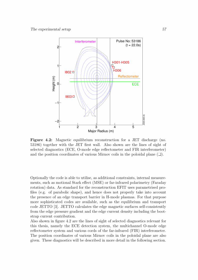
JET is to date the world’s largest tokamak. It produced its first plasma in June1983. Since January 2000 the scientific programme is conducted by researchersfrom associations all over Europe in the framework of the European Fusion De-velopment Agreement (EFDA).Figure 4.1 shows an overview of the JET device, together with some typicalplasma parameters. The toroidal magnetic field is produced by a set of 32 D-shaped coils. Inductive coupling between the primary winding and the toroidalplasma is supported by the massive eight limbed transformer core. Around theoutside of the vacuum vessel, a set of six poloidal magnetic field coils (outerpoloidal field coils) is used for positioning, shaping and stabilising the positionof the plasma inside the vessel.The NBI heating system (not shown in the figure) consists of two racks of injec-tors capable of delivering a total of 17 MW (recently upgraded to 23 MW) intothe plasma for 10 s at injection energies up to 140 keV. The fast particles areinjected tangentially into the plasma, in standard mode of operation in the samedirection as the plasma current (co-injection). After field and current reversal,counter-injection is also possible. Nominally up to 32 MW of ICRH heating arealso available, but since the coupling efficiency is low in the presence of type-IELMs, in practice not more than 4-8 MW are usually delivered into the plasma.The ICRH antennas can be operated as a phased array for current drive studies.LHCD is also available at JET. The generators are capable of delivering up to 12MW for 10 s. In practice, the power effectively coupled to the plasma dependson the plasma conditions.Figure 4.2 shows a magnetic equilibrium reconstruction for a typical JET dis-charge, calculated by the equilibrium code EFIT [1, 2]. EFIT reconstructs theMHD equilibrium of JET plasmas, i.e. plasma shape, current profiles, etc. usingthe Grad-Shafranov equation constrained by external magnetic measurements.

56 Chapter 4

Figure 4.1: Layout of the JET device, together with some typical plasma pa-rameters.

The experimental setup 57

Interferometer

ECE

Reflectometer

I802

I803

H301-H305

H306

2

1

0

-1

-2

2 3 4 51

Heig

ht (

m)

Major Radius (m)

JG

03

.66

3-2

c

Pulse No: 53186 (t = 22.0s)

Figure 4.2: Magnetic equilibrium reconstruction for a JET discharge (no.53186) together with the JET first wall. Also shown are the lines of sight ofselected diagnostics (ECE, O-mode edge reflectometer and FIR interferometer)and the position coordinates of various Mirnov coils in the poloidal plane (�).

Optionally the code is able to utilise, as additional constraints, internal measure-ments, such as motional Stark effect (MSE) or far-infrared polarimetry (Faradayrotation) data. As standard for the reconstruction EFIT uses parametrised pro-files (e.g. of parabolic shape), and hence does not properly take into accountthe presence of an edge transport barrier in H-mode plasmas. For that purposemore sophisticated codes are available, such as the equilibrium and transportcode JETTO [3]. JETTO calculates the edge magnetic surfaces self-consistentlyfrom the edge pressure gradient and the edge current density including the boot-strap current contribution.Also shown in figure 4.2 are the lines of sight of selected diagnostics relevant forthis thesis, namely the ECE detection system, the multichannel O-mode edgereflectometer system and various cords of the far-infrared (FIR) interferometer.The position coordinates of various Mirnov coils in the poloidal plane are alsogiven. These diagnostics will be described in more detail in the following section.

58 Chapter 4

Figure 4.3: A Mirnov coil from the high resolution array installed at JET. Thecoils are wound from titanium wire in a single layer onto an alumina ceramicformer with a return wire through the center of the coil.

4.2 JET diagnostics relevant for this thesis

4.2.1 Mirnov coils

Mirnov coils pick up fluctuations of Bθ (better: changes of the poloidal magneticflux through the coil,

∫

Bθ dA), and are used as a standard MHD diagnosticon almost all tokamak devices. The coils are installed within the vacuum ves-sel close to the plasma boundary. By making measurements at different poloidaland toroidal locations the structure of magnetic field perturbations can be deter-mined, as well as their amplitude and frequency. Since magnetic coils detect thetime derivative of B (Faraday’s law), for a given mode amplitude the detectedamplitude of the oscillations on the Mirnov signal will be proportional to thefrequency f of the mode. This implies that, in principle, the higher the modefrequency is, the more sensitive the Mirnov diagnostic becomes for that mode.However, technical constraints such as the finite sampling rate of the signal orthe finite capacitance of the coil circuit will impose an upper limit on the highestdetectable frequency of oscillations.On JET a number of coil arrays with high frequency response are available. Thepoloidal distribution of the coils is shown in figure 4.2. The coils are designedfor high frequencies up to 500 kHz (figure 4.3).For this thesis two sets of Mirnov coils are relevant: a set of five coils at samepoloidal angles but at different toroidal locations (labelled in figure 4.2 as H301-H305, table 4.1), and a set of four coils at nearly the same toroidal angle at

The experimental setup 59

Coil R(m) Z(m) φ(◦)H301 3.881 1.001 -13.0H302 3.881 1.013 2.94H303 3.881 1.005 13.11H304 3.880 1.045 18.74H305 3.882 1.007 20.38

Table 4.1: Coordinates of the toroidal set of Mirnov coils H301-H305, for thestandard vessel temperature of 200 ◦C.

different poloidal locations around the plasma (coils I802, I803, H304 and H306in figure 4.2). Coils H304 and H306 are poloidally 6 degrees apart, while coilsI802 and I803 are 50 degrees apart.The data is collected for selected time windows in the discharge with either 250kHz or 1 Mhz sampling rate, thus allowing for the study of modes with up to 125or 500 kHz frequency (Nyquist frequency limit), respectively. In addition, thereis a signal from a single Mirnov coil, sampled at 250 kHz, available throughoutthe whole discharge.

4.2.2 Electron cyclotron emission

The measurement of electron cyclotron emission (ECE) is a passive techniquethat under certain circumstances can be used to determine the local electrontemperature Te(r) in the plasma. The theory of ECE emission is well understood[4], and its capabilities for measuring Te are used routinely on almost every fusiondevice.The electrons of a magnetically confined plasma gyrate around the field lines andas a consequence emit electromagnetic radiation at their cyclotron frequency

ωce =eB

γme

(where γ is the relativistic factor) and its harmonics (ω = nωce, with n = 1, 2 ...).The EC waves can propagate in two modes of polarisation perpendicular to themagnetic field in the plasma: as Ordinary (O-mode) waves and eXtraordinary (X-mode) waves. O-mode waves have their electric field vector pointing parallel to

the magnetic field in the plasma ( ~E ‖ ~B), while for X-mode waves ~E ⊥ ~B. On itspath towards the receiving antenna, EC waves with frequency ω are continuouslyemitted and reabsorbed by particles in the plasma resonant at that frequency.The final intensity of EC radiation emitted by the plasma is a convolution of theemission and absorption processes taking place in the plasma

I(ω) =

∫

βω(l) exp

[

−∫

l

αω(l′) dl′]

dl

60 Chapter 4

Figure 4.4: Sketch of emission, β, and transmission, e−τ , and emitting profiles(from [5]).

where βω and αω are the emission and absorption coefficients, respectively. Thequantity τ(l) ≡

∫

lαω(l′) dl′ is known as the optical depth, and e−τ as the trans-

mission coefficient. For thermal plasmas the emission and absorption coefficientsare proportional (Kirchhoff’s law of radiation)

βω(~r) =(ω

c

)2 Te(~r)

(2π)3αω(~r)

Thus, when the distribution function of the electrons is Maxwellian, the emit-ted intensity I(ω) is related to the electron temperature. For plasma conditionswhere a certain harmonic (and propagating mode) of the electron cyclotron res-onance is highly absorbed (the transmission coefficient is very low, or the opticaldepth is very high) the variation of the transmission coefficient has a peakedshape around the resonance region (see figure 4.4). Hence, for optically thickplasmas the emitted intensity is a measure of the local electron temperature inthat region.The EC absorption coefficient, α, is a complicated function depending on theharmonic, the mode of propagation and the plasma parameters (density andtemperature). Generally, the best absorbed harmonics and modes are the 1stharmonic O-mode and the 2nd harmonic X-mode. For these modes the absorp-tion coefficient increases linearly with the density and more than linearly with thetemperature. Thus the plasma should be hot and dense enough to be opticallythick. These conditions are not necessarily fulfilled in certain plasma regions, i.e.the plasma edge.

The experimental setup 61

On JET an array of 48 (recently upgraded to 96) ECE heterodyne radiometerchannels is available, viewing the plasma horizontally from the low field side,slightly below the plasma midplane (figure 4.2). The total range of frequenciesthat can be measured is 70-140 GHz, but only a subrange of frequencies is se-lected for operation in a discharge. The frequencies are usually selected suchthat the ECE channels have their resonance on the low field side, and hence thetemperature profile on the outboard midplane is measured. From the receivingantenna on the low field side of the vessel the waves are transmitted to an ac-quisition system through ∼ 40 m long oversized waveguides. First a polarisationswitch is used to switch from O- to X-mode operation. Then the signal is passedon to a set of two (out of six available) downconverters. To adjust the range ofradii to be covered an algorithm controls the polarisation switch and selects theappropriate downconverters depending on the toroidal magnetic field of the dis-charge. The downconverters consist of a local oscillator and a mixer. The mixerproduces lower and upper sidebands, from which the upper side band is selected(the lower sideband is suppressed by filters). The outcoming signal then has afrequency of 6-18 GHz. From each downconverter the signal is passed on to a lownoise amplifier and a splitter, which splits the signal into 24 individual channels500 MHz apart. Each of these channels passes through a filter bank with 250MHz bandwidth. The signals are then demodulated by Schottky diodes. Theoutcoming voltage is proportional to the radiation temperature of the plasma.After passing through a number of amplifiers the resulting DC signal is finallydigitised in an ADC. The absolute calibration of the ECE signals is done throughcross-calibration with a Michelson-Interferometer.ECE data with a frequency response of 1 kHz is available throughout the dis-charge, while for selected time windows fast ECE data with 250 kHz samplingrate is available as well.

4.2.3 O-mode reflectometer

The use of reflectometry [6] is based on the reflection of electromagnetic wavesin a plasma. In general, a reflectometer consists of a probing beam (O-mode orX-mode waves) propagating through the plasma and a reference path outsidethe plasma (see figure 4.5). In the following only the case of O-mode waves isdiscussed (X-mode reflectometry has not been used within this thesis).For O-mode waves total reflection occurs at the critical density nc when the wavefrequency, ω, equals the plasma frequency, ωpe, defined as

ωpe(R) =

(

e2ne(R)

ε0me

)1/2

62 Chapter 4

Figure 4.5: A schematic representation of a microwave reflectometer [6].

The microwave beam probing the plasma will undergo a phase shift with respectto the beam in the reference arm. This phase difference is given by [7]

∆ϕ = 2ω

c

∫ Rant

Rc

(

1 −ω2

pe(R)

ω2

)1/2

dR − π

2+ω

c(Ls − Lr)

where Rc is the position of the reflecting layer in the plasma, Rant is the positionof the launching antenna, Ls is the length of the waveguides of the signal arm toand from the antenna, and Lr is the length of the waveguides used in the refer-ence arm. Thus, when the source frequency is held constant, a reflectometer willmeasure changes in the phase difference between the signal path and referencepath as a result of variations in the electron density.Since the set up of the O-mode reflectometer at JET has changed repeatedlyover time, here only the configuration relevant for this thesis will be discussed.The system consists of ten channels probing densities from 0.4-6.0 × 1019 m−3.Thus, it can perform simultaneous measurements of density fluctuations at tenradial positions. The distribution of channel frequencies and respective cut offdensities is given in table 4.2. The plasma is probed from the low field sidealong the midplane of the torus (figure 4.2). Due to the relatively low probingdensities, in H-mode most, if not all, channels have their cut off at pedestal radii.This converts the JET O-mode reflectometer into a valuable tool for studyingdensity fluctuations at the edge transport barrier.The waves are generated by voltage-controlled Gunn diodes at different frequen-cies and combined into a single oversized waveguide. Separate launching andreceiving antenna are used to avoid spurious reflections. The phase changes forfluctuation analysis are measured by a coherent detector system (equivalent toa homodyne detector). For each channel phase variations are acquired with aphasemeter at a maximum time resolution of 2 µs.

The experimental setup 63

Frequency DensityChannel (GHz) (1019 m−3)

1 18.6 0.432 24.3 0.733 29.2 1.064 33.8 1.425 39.5 1.946 45.2 2.537 50.3 3.148 57.1 4.059 64.2 5.1110 69.5 6.00

Table 4.2: Frequencies and cut off densities of the multichannel O-mode reflec-tometer at JET.

4.2.4 FIR interferometer

Laser interferometry for measuring electron density has become a standard di-agnostic tool on most tokamaks. When a coherent O-mode wave passes throughthe plasma the wave undergoes a change in its phase with respect to a referencebeam running in vacuum, due to the finite refractive index of the plasma. Atfrequencies which are large compared with the plasma frequency, the change inthe phase of the beam is proportional to the electron density integrated alongthe beam probing the plasma

∆ϕ =e2

4πε0mec2λ

∫

nedl

where λ is the vavelength of the radiation. This phase difference can be measuredby a Mach-Zehnder interferometer arrangement as shown in figure 4.6.A multichannel FIR interferometer has been used on JET routinely since 1984 [9].The system presently consists of four vertical and 4 lateral (oblique) viewingcords. For the purpose of this thesis only the two vertical cords shown in figure4.2 are of interest, which measure the line-integrated density in the plasma coreand at the plasma edge. The instrument is of the Mach-Zehnder type, with aheterodyne detection system. The basic source is a DCN (deuterium cyanide)laser operated at 195 µm. A modulation frequency of 100 kHz is produced bydiffraction from a rotating grating (3600 groves rotating at 28 Hz). The inputbeams are then transferred by free optical propagation through the basement,passing below the biological shield, into the torus hall. The optics in the torus hallis situated in a large C frame (tower) of ∼ 52 tons of weight, independent fromthe machine, to minimise the influence on vibrations on the phase measurement.

64 Chapter 4

Figure 4.6: Schematic layout of a Mach-Zehnder interferometer [8]. The beamsare split into a probing and a reference beam, and are recombined with a fre-quency shifted beam before reaching the detectors. The beat frequency is chosento be sufficiently high to allow a good time resolution in the phase measurement,and sufficiently low to be electronically tractable. The phase differences ϕr andϕp reflect the different pathlengths whereas ∆ϕ is caused by the refractive effectsof the plasma.

The probing beams which arrive in the torus hall are split up into individualchannels. A half-wave plate rotates the beam polarisation so that it arrives at theplasma as O-mode wave. One part passes through the plasma and is recombinedwith the corresponding modulated channels afterwards. The other part is sentback without going through the plasma and recombined with a portion of themodulated beam to constitute the reference beam. On the return path intothe diagnostic hall the beams are directed into oversized dielectric waveguides.There, high sensitivity InSb (indium antimonide) He-cooled detectors are used,which allow to perform the the phase shift measurement with an accuracy of 1/20of a fringe, corresponding to a line-integrated electron density of 5 × 1017m−2.The total distance between laser and detectors is ∼ 80 m.The interferometer data is acquired throughout the discharge with a maximumtime resolution of 0.5 ms (faster data for MHD analysis purposes is not usedroutinely). The data needs to be further validated and corrected for fringe jumps(∆ϕ = 2π). Such fringe jumps can occur when sudden events occur in theplasma, for instance large ELMs or the injection of a pellet. The fringe jumpcorrection is done semi-automatically with the aid of an algorithm.

The experimental setup 65

4.2.5 Soft X-ray cameras

Plasma radiation in the soft X-ray wavelength (∼ 0.1 - 2 nm) can be detectedby silicon diodes. The diodes are located in pinhole cameras, viewing the plasmafrom various angles. They measure the X-ray emission above a threshold energydetermined by a thin metallic foil placed in front of the detectors. This way,core or edge radiation can be selected. Each channel yields the line-integratedradiation along the line of sight of the particular diode. Silicon diodes have avery fast time response, typically a fraction of a microsecond. Thus, soft X-raycameras are well suited for the analysis of fluctuations in the plasma, and areroutinely employed for MHD analysis purposes.In a fusion plasma, there are mainly two sources of soft X-ray radiation: Line-radiation from medium-Z impurities in the plasma core, and continuum radiationfrom bremsstrahlung. For soft X-ray measurements continuum emission is used.The wavelength range for the measurements is chosen such as to minimise theinfluence of line-radiation. The soft X-ray flux is sensitive to fluctuations of theelectron temperature, electron density and effective charge of the plasma (Zeff).The latter is defined as

Zeff =

∑

j njZ2j

∑

j njZj

where the sum goes over all the ion species in the plasma. The (frequency-

integrated) flux emitted locally in the plasma scales roughly with n2eT

1/2e Zeff .

On JET several soft X-ray cameras were originally installed, but most of theirdiodes were damaged by neutrons in past D-T campaigns. This triggered the in-stallation of a pair of radiation hardened soft X-ray cameras [10,11], which wereavailable for this thesis. The two cameras each contain 17 detector assembliesembedded into a large concrete shield with the detectors viewing the plasmathrough stainless steel collimators and 250 µm Be windows. The cameras mea-sure radiation in the wavelength range 0.15-2 nm. They are installed at differenttoroidal locations (octants 4 and 8 of the torus), with same lines of sight in apoloidal cross section, viewing the plasma from the outboard side. The lines ofsight are shown in figure 4.7. The fast soft X-ray data is acquired with 250 kHzsampling rate and is available for selected time windows during the discharge.

4.3 Data analysis methods used in this thesis

Signals suitable for the MHD analysis of discharges require a high sampling ratein order to be able to resolve the fluctuations associated with the occurrence ofinstabilities. Thus, the analysis unavoidably involves processing of large amountsof data. It becomes important to employ efficient means of looking at the data.For this purpose a number of codes for standard MHD analysis of discharges are

66 Chapter 4

Figure 4.7: Lines of sight of the radiation hardened soft X-ray camera.

available at JET. In addition, an extensive collection of Matlab-based routineshas been developed within this thesis, well suited for multipurpose MHD analysis,but also adapted to the specific requirements that have been arising during thethesis. The code, which has been named JETMHD, is still under continuousdevelopment and presently spans about 6000 lines of Matlab code. The JETMHDcode led to the identification of various phenomena such as the ELM precursorsdiscussed in chapter 5, and most of the material presented in chapters 5 and 6has been processed with it.In the following a number of signal processing methods routinely employed inthis thesis are outlined.

4.3.1 Spectrograms

Spectrograms are colourmapped images in which every Fourier component of thesignal is plotted as a dot in the plane of frequency versus time, and representedby a colour indicating its amplitude. It is convenient to use spectrograms withlogarithmic colour scales, as this allows modes spanning many orders of magni-tude in amplitude to be displayed. An example of a spectrogram plot can befound in figure 5.2 on page 78.The original signal is first time-windowed into groups of nFFT = 2N samples,where N is a user-determined integer. The optimum value for N depends on the

The experimental setup 67

sampling rate of the signal, e.g. for signals with 250 kHz sampling rate N = 8-10(i.e. 256 to 1024 points per time window) is usually a reasonable choice. Insteadof windowing the signal with a box function, it is usually better to use a (bellshaped) Hanning window (this method truncates the data at the beginning andend of the time window in a smoother way). The coefficients of the Hanningwindowing function are computed by the following equation

wk =1

2

[

1 − cos

(

2πk − 1

nFFT − 1

)]

k = 1, ..., nFFT (4.1)

in which k indicates the index of the sample point in the window. The distancebetween time windows is nFFT/2 samples, hence there is an overlap. Each win-dow is then fast-fourier-transformed (FFT) to give amplitude as a function offrequency for that particular time interval.Both the time and the frequency resolution of an FFT-based spectrogram arelimited by the “Fourier Uncertainty Principle”

∆fFFT∆tslice = 1

which is simply a mathematical property of the discrete Fourier transform. In-creasing the time resolution of a spectrogram, which is done by decreasing nFFT

(i.e. N), comes at the expense of a reduced frequency resolution (a higher∆fFFT). This is because the frequency resolution of the FFT is the samplerate divided by the number of samples in the slice (∆fFFT = fsample/nFFT).There are other alternatives to the FFT-based spectrograms, which have beenoccassionally used within this thesis. Wavelet analysis uses a windowing tech-nique with variable sized regions. It allows the use of long time intervals wheremore precise low frequency information is needed, and shorter time intervals forhigh frequency information.

4.3.2 Toroidal mode number determination

It has been mentioned previously that instabilities usually rotate and have heli-cal mode structure. By analysing the relative phase shift of fluctuations pickedup by a set of toroidally distributed Mirnov coils, the toroidal mode number nassociated with these fluctuations can be deduced.Starting from the signals measured by the various coils, the signals are firstfast-fourier-transformed in a similar way as for the spectrogram. This yieldsamplitude and phase behaviour as a function of time and frequency for each ofthe signals. To reduce the computational effort, points for which the Fourier am-plitude is below a user-defined threshold (“background noise”) are disregarded.Since the phase obtained from the Fourier analysis is in the range from −π to+π, it is necessary to correct for jumps (larger than π) in the relative phase offluctuations from coil to coil. To that purpose a build-in Matlab function called

68 Chapter 4

−0.3 −0.2 −0.1 0 0.1 0.2 0.3 0.4−3

−2

−1

0

1

2

3

Toroidal Angle φ [rad]

Flu

ctua

tion

Pha

se α

[rad

]

Pulse No 53062: t = 62.3542 s, f = 18.07 kHz, n = 8.2, fit−error = 0.38

H301

H302

H303

H304

H305

fit

Figure 4.8: Example of a linear fit procedure to obtain the toroidal modenumber n. In this case, the nearest integer number to the fit value of 8.2 is 8.

unwrap exists. Given the phases αj(t, f) of the fluctuations for each time andfrequency and the toroidal coordinates φj of the coils, the toroidal mode numbern is in principle given by the “slope”:

n = ∆α/∆φ (4.2)

Thus, for each time and frequency the corresponding n can be obtained by per-forming a least squares linear fit of the unwrapped phases αj versus φj. As anillustrative example, figure 4.8 shows the result of such a fitting procedure. Allthe values for t and f are scanned, and the fitting procedure is performed manythousand times until all the points for the plot are computed. To further re-duce the noise level of the plots, points are discarded if the fitting error exceedsa certain user-defined threshold, although in practice this option did not provereally necessary. Finally, the n-numbers obtained for each time and frequencyare mapped into a colour scheme and plotted versus t and f (without roundingto the nearest integer), in a similar fashion as spectrograms. An example of sucha mode number spectrum can be found in figure 5.3 on page 79. In practice,one cannot reliably determine a mode number from a single data point in thespace of time and frequency, but all the points corresponding to a given modegenerally show up with nearly identical mode numbers, and one can be confidentthat the mode number is correct.The range of mode numbers which can be determined is restricted by the limita-tion that the phase jump ∆α between probes separated by a toroidal angle ∆φ

The experimental setup 69

cannot be greater than π. From equation (4.2) the phase jump ∆α is equivalentto n∆φ, so the upper limit for n is given by

|n| ≤ π/|∆φ|

Hence, for a given set of coils the maximum n that can be correctly determined ispredefined by the largest gap between two coils. For the five coils of the toroidalarray available on JET (H301-H305) the largest gap is ∼ 16◦ (between H301 andH302). Thus, this set is suitable for modes with |n| ≤ 11. A subset of coils withlower ∆φ (e.g. H302-H305) can be employed if higher mode numbers need to beresolved, or simply to check the correctness of previous calculations.

4.3.3 Poloidal mode number determination

Although the underlying idea is the same as for toroidal mode numbers, thedetermination of poloidal mode numbers, m, on the basis of poloidally distributedcoils is more complicated because the poloidal symmetry is broken due to thetoroidicity of the magnetic flux surfaces. The slope of the magnetic field linesvaries poloidally, resulting in a poloidal variation of the wavelength of the mode,which is larger at the outer (low field) side of the torus. Hence, the apparent mnumber depends on the poloidal angle where the coils are located (so called θ∗-effect [12,13]). For the case of a circular cross section this effect can be describedto first order of the inverse aspect ratio by a transformation from θ to θ∗

θ∗ = θ −(

βp +li2

+ 1

)

ε sin θ

where βp is the poloidal beta, li is the internal inductance of the plasma andε = r/R0 is the inverse aspect ratio. Plasma shaping (elongation, triangularity)and the presence of an X-point impose further difficulties, in particular for modeslocated close to the plasma boundary. The X-point will distort the poloidal modestructure in such a way that coils picking up magnetic fluctuations around theplasma midplane (θ = 0, π) will have the tendency to measure a too low m-number.Only a limited numbers of coils, distributed poloidally around the plasma crosssection, are available on JET. For the analysis 4 coils are used, two on the lowfield side (H304 and H306, which are 6 degrees apart), and two on the high fieldside (I802 and I803, 50 degrees apart). Equilibrium calculations have shownthat on JET the pitch of the field lines at the torus high field side is close tothe average pitch of field lines of the magnetic surfaces [14]. Hence, m-numbersdetermined from coils at the high field side can be taken as an approximation forthe true m-number of the modes. The phase difference obtained from the closelyspaced coils H304 and H306 at the low field side is used to correct for possiblephase jumps in the phase difference for the two coils on the high field side. Due

70 Chapter 4

to aliasing effects the set of coils is not suitable for the analysis of modes withhigh m numbers. However, for lower m (� 6) the m-number determination hasproven reasonably reliable and is routinely used on JET since a number of years.

4.3.4 Coherence analysis

Coherence analysis is a general signal processing technique that can provide fur-ther insight into the signal behaviour. It proves to be a very valuable tool inparticular for situations in which signals are dominated by noise. In the contextof this thesis it is used to obtain information about the radial mode structure ofinstabilities, specifically about the radial phase behaviour of oscillations and theradial displacement profile ξr(r). In principle, the same information could be ob-tained through straightforward Fourier decomposition. However, the coherenceanalysis is superior to it in terms of noise reduction. An example of a coherenceanalysis can be found in figure 5.6 on page 84. Before going into the details ofthe analysis, it is worth to shortly review some of the signal processing conceptsfirst.The true cross-correlation sequence is a statistical quantity defined as

Rxy(m) = E[xn+my∗n] (4.3)

where xn and yn are stationary random processes, ∗ stands for the complexconjugate, −∞ < n < +∞, and E[ · ] is the expected value operator. Inpractice, Rxy must be estimated, because it is only possible to access a finitesegment of the infinite-length random process. A common estimate based on Nsamples of xn and yn is the deterministic cross-correlation sequence (also calledtime-ambiguity function)

Rxy(m) =

N−m−1∑

n=0

xn+my∗m

R∗yx(−m)

for m ≥ 0

for m < 0(4.4)

The power spectral density, Pxx, of x is defined as

Pxx(ω) =1

2π

+∞∑

m=−∞

Rxx(m) e−iωm (4.5)

where here ω denotes the normalised frequency, ω = 2πf/fs (fs is the samplingrate). Thus, Pxx(ω) is related to the autocorrelation sequence of x through thediscrete Fourier transform. It can be easily shown that Pxx(ω) is a real quantity.It represents the power content of a signal in an infinitesimal frequency band. Inanalogy to (4.5), the cross spectral density of two signals x and y is given by

Pxy(ω) =1

2π

+∞∑

m=−∞

Rxy(m) e−iωm (4.6)

The experimental setup 71

In general, Pxy(ω) is complex. A related quantity is the magnitude squaredcoherence function, which is defined as

Cxy(ω) =|Pxy(ω)|2

Pxx(ω)Pyy(ω)(4.7)

Cxy(ω) is a real number between 0 and 1 and represents a measure for the spec-tral correlation of fluctuations present in signals x and y.The routine employed in the context of this thesis calculates the spectral densitiesPxx, Pyy and Pxy using Welch’s method [15]. The signals are first time-windowedin a similar fashion as for the spectrogram. The signal section to be analysedis then segmented again into eight overlapping sections of equal length. Eachof these segments is then windowed with a Hanning window of same length asthe segment. The spectral densities (and with them the coherence function) arecomputed directly from the signal sections with FFT, and the result is then av-eraged over all eight segments.As mentioned above, the coherence analysis is used to obtain information aboutthe radial structure of a mode. To this purpose, a preferably clean reference sig-nal (e.g. from the magnetics) is chosen, and the coherence and the cross spectraldensity of that signal with other signals (e.g. a set of ECE or reflectometer chan-nels) is calculated, for a given time window, at all frequencies. The distributionof the phase of the cross-spectral density (remember that Pxy is complex) acrossthe channels is used to obtain information about the radial phase behaviour ofthe mode oscillations.For the calculation of the radial displacements it is assumed that all spectra arecomposed of a constant background and a Gaussian function over the frequencyrange of interest. The spectrum of the reference signal of the coherence calcula-tion is used to obtain the central position and the width of the Gaussian visiblein the frequency range of interest. The spectra of each of the diagnostic channelsin the relevant frequency interval is then fitted with a Gaussian of the width andcentral position of the reference spectrum and a background directly obtainedfrom the power spectrum of the channel. The amplitude A of the fluctuations(e.g. in the case of ECE data, A corresponds to ∆Te(f)) is then [14]

A = 2√

2π(A0 − b)s

where the factor two is to compensate for the Hanning window function (whoseaverage value is 0.5, see equation (4.1)), A0 is the peak value of the Gaussianfit, b is the background, and s = 0.4247 × FWHM (full width half maximum)of the Gaussian fit made to the reference spectrum. Each fit is determined byfour parameters: A0, b, s and the central position f0. Their standard deviationis used to estimate the error bars for the amplitude. In practice only A0 and bcontribute to the error bars if the reference signal is well chosen. Each oscillationcycle with amplitude A leads to a maximum and a minimum of the local radial

72 Chapter 4

profile of the diagnostic in question. The radial distance between points of equaltemperature in the maximum and minimum profiles yields the displacement.

References

[1] Lao L L, John H St, Stambaugh R D, Kellman A G, and Pfeiffer W 1985Nucl. Fusion 25 1611

[2] O’Brien D P et al 1992 Nucl. Fusion 32 1351

[3] Cenacchi G, Taroni A 1988 Rapporto ENEA RT/T1B 88 (5)

[4] Bornatici M, Cano R, de Barbieri O, and Engelmann F 1983 Nucl. Fusion23 1153

[5] Tribaldos V 2001 EFDA-JET-PR(01) 44

[6] Laviron C, Donne A J H, Manso M E, and Sanchez J 1996 Plasma Phys.Control. Fusion 38 905

[7] Sips A C C and Kramer G J 1993 Plasma Phys. Control. Fusion 35 743

[8] Wesson J A 1997 Tokamaks (Clarendon Press: Oxford)

[9] Braithwaite G et al 1989 Rev. Sci. Instrum. 60 2825

[10] Gill R D, Alper B, Edwards A W and Dillon S, JET-IR(95)03

[11] Gill R D, Alper B and Edwards A W 1997 JET-R(97)11

[12] Merezhkin V G 1978 Sov. J. Plasma Phys. 4 152

[13] Klueber O et al 1991 Nucl. Fusion 31 907

[14] Smeulders P et al 1999 Plasma Phys. Control. Fusion 41 1303

[15] Welch P D 1967 IEEE Trans. Audio Electroacoust. AU-15 70