Embed Size (px)
Citation preview

Lecture Notes of Statistical 517, Chapter 4
Chapter 4: Some ElementaryStatistical Inferences
Tonglin Zhang
Tonglin Zhang, Department of Statistics, Purdue University Chapter 4: Some Elementary Statistical Inferences

4.1 Sampling and Statistics
4.1 Sampling and Statistics
(Random Sample) X1, · · · ,Xn constitute a random sample on X ifX1, · · · ,Xn are iid with the same distribution as that of X . Theyhave the same
I expected values (means): E(X1) = · · · = E(Xn) = µ
I variances: V(X1) = · · · = V(Xn) = σ2.
Tonglin Zhang, Department of Statistics, Purdue University Chapter 4: Some Elementary Statistical Inferences
4.1 Sampling and Statistics
I In theoretical statistics, we use random variables to representobservations (i.e., data). Then, we can use probability tostudy their properties.
I In applied statistics, we use values. We look at their numericalresults.
Tonglin Zhang, Department of Statistics, Purdue University Chapter 4: Some Elementary Statistical Inferences
4.1 Sampling and Statistics
A statistic is a function of data. It becomes a real number afteryou have data.
I Before collecting the data, it is a random variable. Intheoretical statistics, we treat it as a random variable.
I After collecting the data, it is a number. In applied statistics,we treat it as a number.
Tonglin Zhang, Department of Statistics, Purdue University Chapter 4: Some Elementary Statistical Inferences

4.1.1. Point Estimators
4.1.1. Point Estimators
Three main problems in statistics.
I Point estimation. The answer is a real number. There arethree terms
I Estimation. The entire method for the formula. It is the mostimportant step in the derivation of the three main problems.
I Estimator. The formula (must be a statistic).I Estimate. A value. After you have data, an estimator becomes
an estimate.
I Confidence interval. The answer is an interval, such as a± bor [L,U].
I Hypothesis testing. The answer is True or False.
Tonglin Zhang, Department of Statistics, Purdue University Chapter 4: Some Elementary Statistical Inferences
4.1.1. Point Estimators
Biased versus Unbiased
Suppose we use T = T (X1, · · · ,Xn) to estimate θ.
I If E(T ) = θ, then we call it is unbiased;
I otherwise, we called E(T )− θ as the bias of T .
Criticism: T 2 is not an unbiased estimator of θ2 even if T is anunbiased estimator of θ.
Tonglin Zhang, Department of Statistics, Purdue University Chapter 4: Some Elementary Statistical Inferences

4.1.1. Point Estimators
If X1, · · · ,Xn are random sample with common PDF (or PMF)f (x) and CDF F (x), then the joint PDF (or PMF) is
fX1,··· ,Xn(x1, · · · , xn) =n∏
i=1
f (xi )
and the joint CDF is
FX1,··· ,Xn(x1, · · · , xn) =n∏
i=1
F (xi ).
Tonglin Zhang, Department of Statistics, Purdue University Chapter 4: Some Elementary Statistical Inferences

4.1.1. Point Estimators
If a parameter is contained in f (x) so that we can write
f (x) = fθ(x),
then the likelihood function is defined by their joint PDF (or PMF)as
L(θ) =n∏
i=1
fθ(Xi ).
Tonglin Zhang, Department of Statistics, Purdue University Chapter 4: Some Elementary Statistical Inferences
4.1.1. Point Estimators
I The likelihood function is identical to the joint PDF or PMF.
I The focus is the parameter but not the distribution.
I The maximum likelihood is the most important method.
I A main step in the maximum likelihood approach is thederivation of the maximizer.
I Maximum likelihood approach has also been extended tomany cases.
I If θ is the MLE of θ, then for any continuous function g(·),g(θ) is also the MLE of g(θ).
Tonglin Zhang, Department of Statistics, Purdue University Chapter 4: Some Elementary Statistical Inferences
4.1.1. Point Estimators
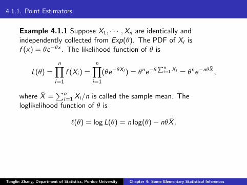
Example 4.1.1 Suppose X1, · · · ,Xn are identically andindependently collected from Exp(θ). The PDF of Xi isf (x) = θe−θx . The likelihood function of θ is
L(θ) =n∏
i=1
f (Xi ) =n∏
i=1
(θe−θXi ) = θne−θ∑n
i=1 Xi = θne−nθX ,
where X =∑n
i=1 Xi/n is called the sample mean. Theloglikelihood function of θ is
ℓ(θ) = log L(θ) = n log(θ)− nθX .
Tonglin Zhang, Department of Statistics, Purdue University Chapter 4: Some Elementary Statistical Inferences
4.1.1. Point Estimators
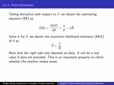
Taking derivative with respect to θ, we obtain the estimatingequation (EE) as
ℓ(θ) =∂ℓ(θ)
∂θ=
n
θ− nX .
Solve it for θ, we obtain the maximum likelihood estimator (MLE)of θ as
θ =1
X.
Note that the right side only depends on data. It will be a realvalue if data are provided. This is an important property to checkwhether the solution makes sense.
Tonglin Zhang, Department of Statistics, Purdue University Chapter 4: Some Elementary Statistical Inferences
4.1.1. Point Estimators
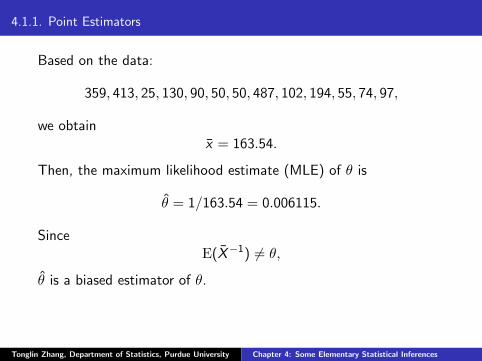
Based on the data:
359, 413, 25, 130, 90, 50, 50, 487, 102, 194, 55, 74, 97,
we obtainx = 163.54.
Then, the maximum likelihood estimate (MLE) of θ is
θ = 1/163.54 = 0.006115.
SinceE(X−1) = θ,
θ is a biased estimator of θ.
Tonglin Zhang, Department of Statistics, Purdue University Chapter 4: Some Elementary Statistical Inferences

4.1.1. Point Estimators
I If I ask you maximum likelihood estimation, you need all ofthose.
I If I ask you maximum likelihood estimator, you need toprovide θ = 1/X .
I If I ask you maximum likelihood estimate, you need to provide0.006115.
Tonglin Zhang, Department of Statistics, Purdue University Chapter 4: Some Elementary Statistical Inferences

4.1.1. Point Estimators
Example 4.1.2. Let X be Bernoulli(θ). Then, X can only be 0 or1. Let θ = P(X = 1). Then, the PMF can be expressed asf (x) = θx(1− θ)1−x . We write X ∼ Bernoulli(θ). Suppose thatX1, · · · ,Xn ∼iid Bernoulli(θ). Then, the likelihood function of θ is
L(θ) =n∏
i=1
θXi (1− θ)1−Xi = θnX (1− θ)n(1−X ).
Tonglin Zhang, Department of Statistics, Purdue University Chapter 4: Some Elementary Statistical Inferences
4.1.1. Point Estimators
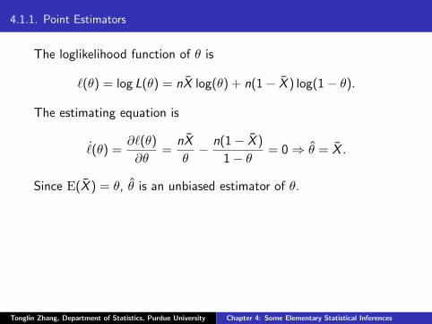
The loglikelihood function of θ is
ℓ(θ) = log L(θ) = nX log(θ) + n(1− X ) log(1− θ).
The estimating equation is
ℓ(θ) =∂ℓ(θ)
∂θ=
nX
θ− n(1− X )
1− θ= 0 ⇒ θ = X .
Since E(X ) = θ, θ is an unbiased estimator of θ.
Tonglin Zhang, Department of Statistics, Purdue University Chapter 4: Some Elementary Statistical Inferences

4.1.1. Point Estimators
Example 4.1.3. Let X1, · · · ,Xn be iid from N(µ, σ2). Then, thePDF is
f (x) =1√2πσ
e−(X−µ)2
2σ2 .
Let θ = (θ1, θ2) = (µ, σ2). The likelihood function of θ is
L(θ) =n∏
i=1
1√2πσ
e−(Xi−µ)2
2σ2
=(1√2π
)n(1
σ2)n2 e−
12σ2
∑ni=1[(X−µ)2+(Xi−X )2].
Tonglin Zhang, Department of Statistics, Purdue University Chapter 4: Some Elementary Statistical Inferences
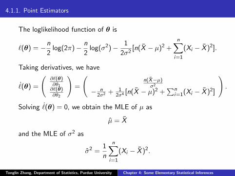
4.1.1. Point Estimators
The loglikelihood function of θ is
ℓ(θ) = −n
2log(2π)− n
2log(σ2)− 1
2σ2[n(X − µ)2 +
n∑i=1
(Xi − X )2].
Taking derivatives, we have
ℓ(θ) =
(∂ℓ(θ)∂θ1∂ℓ(θ)∂θ2
)=
(n(X−µ)
σ2
− n2σ2 +
12σ4 [n(X − µ)2 +
∑ni=1(Xi − X )2]
).
Solving ℓ(θ) = 0, we obtain the MLE of µ as
µ = X
and the MLE of σ2 as
σ2 =1
n
n∑i=1
(Xi − X )2.
Tonglin Zhang, Department of Statistics, Purdue University Chapter 4: Some Elementary Statistical Inferences
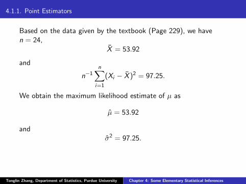
4.1.1. Point Estimators
Based on the data given by the textbook (Page 229), we haven = 24,
X = 53.92
and
n−1n∑
i=1
(Xi − X )2 = 97.25.
We obtain the maximum likelihood estimate of µ as
µ = 53.92
andσ2 = 97.25.
Tonglin Zhang, Department of Statistics, Purdue University Chapter 4: Some Elementary Statistical Inferences
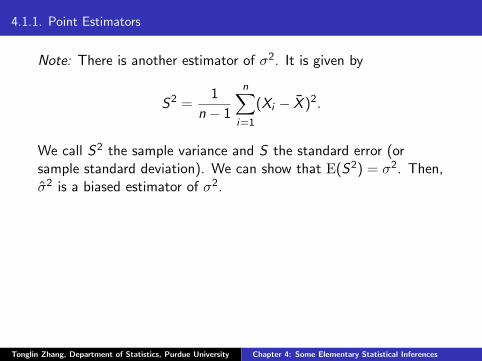
4.1.1. Point Estimators
Note: There is another estimator of σ2. It is given by
S2 =1
n − 1
n∑i=1
(Xi − X )2.
We call S2 the sample variance and S the standard error (orsample standard deviation). We can show that E(S2) = σ2. Then,σ2 is a biased estimator of σ2.
Tonglin Zhang, Department of Statistics, Purdue University Chapter 4: Some Elementary Statistical Inferences

4.1.1. Point Estimators
Example 4.1.4. Let X1, · · · ,Xn be iid from uniform [0, θ]. ThePDF is
f (x) =1
θI (0 ≤ x ≤ θ) =
1/θ, 0 ≤ x ≤ θ,0, otherwise.
The likelihood function is
L(θ) =n∏
i=1
f (Xi ) =n∏
i=1
1
θI (0 ≤ Xi ≤ θ)
=1
θnI (0 ≤ X(1))I (X(n) ≤ θ).
where X(1) = min(Xi ) and X(n) = max(Xi ).Now, we look at the MLE. To make L(θ) large, we need to make θsmall, but θ cannot be lower than X(n). Therefore,
θ = X(n) = max(Xi ).
Tonglin Zhang, Department of Statistics, Purdue University Chapter 4: Some Elementary Statistical Inferences
4.1.1. Point Estimators
Note: We cannot use derivative to find the maximum of thelikelihood function. This example introduces an important methodto find the MLE.
Tonglin Zhang, Department of Statistics, Purdue University Chapter 4: Some Elementary Statistical Inferences

4.1.1. Point Estimators
We next compute the CDF and PDF of X(n). We have a trick. LetF (x) be the CDF of X . Then, F (x) = x/θ if 0 ≤ x ≤ θ. The CDFof X(n) is
Fn(x) =P(X(n) ≤ x)
=P(X1,X2, · · · ,Xn ≤ x)
=n∏
i=1
P(Xi ≤ x)
=F n(x)
=xn
θn.
Tonglin Zhang, Department of Statistics, Purdue University Chapter 4: Some Elementary Statistical Inferences
4.1.1. Point Estimators
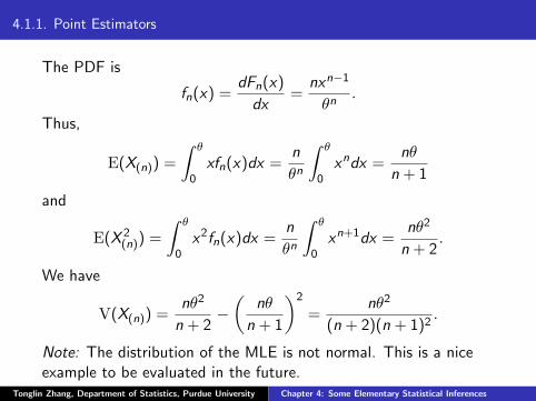
The PDF is
fn(x) =dFn(x)
dx=
nxn−1
θn.
Thus,
E(X(n)) =
∫ θ
0xfn(x)dx =
n
θn
∫ θ
0xndx =
nθ
n + 1
and
E(X 2(n)) =
∫ θ
0x2fn(x)dx =
n
θn
∫ θ
0xn+1dx =
nθ2
n + 2.
We have
V(X(n)) =nθ2
n + 2−(
nθ
n + 1
)2
=nθ2
(n + 2)(n + 1)2.
Note: The distribution of the MLE is not normal. This is a niceexample to be evaluated in the future.
Tonglin Zhang, Department of Statistics, Purdue University Chapter 4: Some Elementary Statistical Inferences
4.1.1. Point Estimators
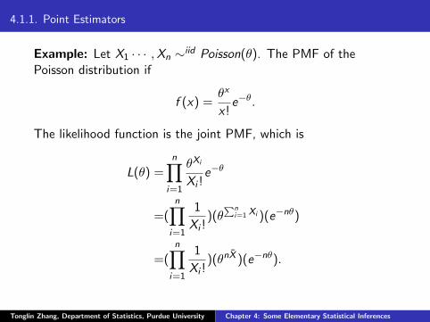
Example: Let X1 · · · ,Xn ∼iid Poisson(θ). The PMF of thePoisson distribution if
f (x) =θx
x!e−θ.
The likelihood function is the joint PMF, which is
L(θ) =n∏
i=1
θXi
Xi !e−θ
=(n∏
i=1
1
Xi !)(θ
∑ni=1 Xi )(e−nθ)
=(n∏
i=1
1
Xi !)(θnX )(e−nθ).
Tonglin Zhang, Department of Statistics, Purdue University Chapter 4: Some Elementary Statistical Inferences
4.1.1. Point Estimators
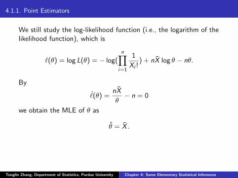
We still study the log-likelihood function (i.e., the logarithm of thelikelihood function), which is
ℓ(θ) = log L(θ) = − log(n∏
i=1
1
Xi !) + nX log θ − nθ.
By
ℓ(θ) =nX
θ− n = 0
we obtain the MLE of θ as
θ = X .
Tonglin Zhang, Department of Statistics, Purdue University Chapter 4: Some Elementary Statistical Inferences
4.2. Confidence Interval
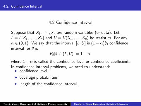
4.2 Confidence Intevral
Suppose that X1, · · · ,Xn are random variables (or data). LetL = L(X1, · · · ,Xn) and U = U(X1, · · · ,Xn) be statistics. For anyα ∈ (0, 1). We say that the interval [L,U] is (1− α)% confidenceinterval for θ is
Pθ[θ ∈ (L,U)] = 1− α,
where 1− α is called the confidence level or confidence coefficient.In confidence interval problems, we need to understand:
I confidence level,
I coverage probabilities
I length of the confidence interval.
Tonglin Zhang, Department of Statistics, Purdue University Chapter 4: Some Elementary Statistical Inferences
4.2. Confidence Interval
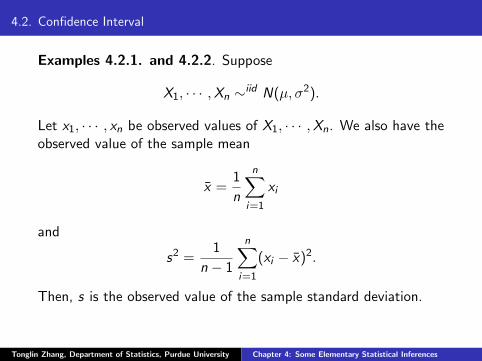
Examples 4.2.1. and 4.2.2. Suppose
X1, · · · ,Xn ∼iid N(µ, σ2).
Let x1, · · · , xn be observed values of X1, · · · ,Xn. We also have theobserved value of the sample mean
x =1
n
n∑i=1
xi
and
s2 =1
n − 1
n∑i=1
(xi − x)2.
Then, s is the observed value of the sample standard deviation.
Tonglin Zhang, Department of Statistics, Purdue University Chapter 4: Some Elementary Statistical Inferences

4.2. Confidence Interval
We have
X ∼ N(µ,σ2
n).
Thus,
P(−zα2≤ X − µ
σ/√n≤ zα
2) = 1− α.
With probability 1− α, there is
−zα2≤ X − µ
σ/√n≤ zα
2.
Tonglin Zhang, Department of Statistics, Purdue University Chapter 4: Some Elementary Statistical Inferences
4.2. Confidence Interval
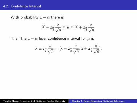
With probability 1− α there is
X − zα2
σ√n≤ µ ≤ X + zα
2
σ√n.
Then the 1− α level confidence interval for µ is
x ± zα2
σ√n= [x − zα
2
σ√n, x + zα
2
σ√n].
Tonglin Zhang, Department of Statistics, Purdue University Chapter 4: Some Elementary Statistical Inferences
4.2. Confidence Interval
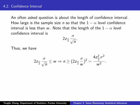
An often asked question is about the length of confidence interval.How large is the sample size n so that the 1− α level confidenceinterval is less than w . Note that the length of the 1− α levelconfidence interval is
2zα2
σ√n.
Thus, we have
2zα2
σ√n≤ w ⇒ n ≥ (2zα
2
σ
w)2 =
4z2α2σ2
w2.
Tonglin Zhang, Department of Statistics, Purdue University Chapter 4: Some Elementary Statistical Inferences

4.2. Confidence Interval
Modification 1. If σ2 is unknown, then we can replace σ2 by s2,leading the large sample confidence interval for µ as
X − zα2
s√n≤ µ ≤ X + zα
2
s√n.
This is recommend if n is large (e.g., n ≥ 40).Modification 2. If n is small, then one suggests to replace zα/2 bytα.2,n−1, leading to
x ± tα2,n−1
s√n.
Tonglin Zhang, Department of Statistics, Purdue University Chapter 4: Some Elementary Statistical Inferences
4.2. Confidence Interval
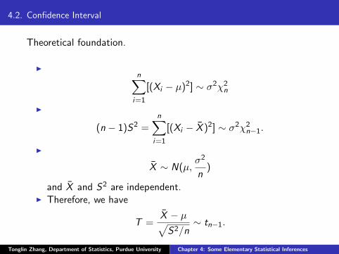
Theoretical foundation.
In∑
i=1
[(Xi − µ)2] ∼ σ2χ2n
I
(n − 1)S2 =n∑
i=1
[(Xi − X )2] ∼ σ2χ2n−1.
I
X ∼ N(µ,σ2
n)
and X and S2 are independent.I Therefore, we have
T =X − µ√S2/n
∼ tn−1.
Tonglin Zhang, Department of Statistics, Purdue University Chapter 4: Some Elementary Statistical Inferences
4.2. Confidence Interval
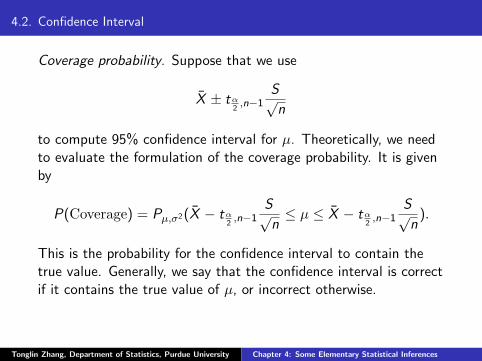
Coverage probability. Suppose that we use
X ± tα2,n−1
S√n
to compute 95% confidence interval for µ. Theoretically, we needto evaluate the formulation of the coverage probability. It is givenby
P(Coverage) = Pµ,σ2(X − tα2,n−1
S√n≤ µ ≤ X − tα
2,n−1
S√n).
This is the probability for the confidence interval to contain thetrue value. Generally, we say that the confidence interval is correctif it contains the true value of µ, or incorrect otherwise.
Tonglin Zhang, Department of Statistics, Purdue University Chapter 4: Some Elementary Statistical Inferences
4.2. Confidence Interval
Equivalently, we have
P(Coverage) = P(−tα2,n−1 ≤
X − µ
S/√n≤ −tα
2,n−1) = 1− α.
I We want to make the value identical to (or close to) 1− α.
I We claim the formulation is bad if it is too high or too low.
I Based on the above result, we conclude that the formulationof t-confidence interval is good.
Tonglin Zhang, Department of Statistics, Purdue University Chapter 4: Some Elementary Statistical Inferences
4.2. Confidence Interval
−1 0 1 2 3
0.0
0.2
0.4
0.6
0.8
1.0
µ
Cov
erag
e P
roba
bilit
y
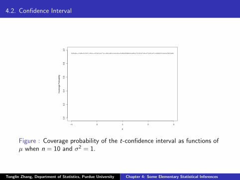
Figure : Coverage probability of the t-confidence interval as functions ofµ when n = 10 and σ2 = 1.
Tonglin Zhang, Department of Statistics, Purdue University Chapter 4: Some Elementary Statistical Inferences

4.2. Confidence Interval
Example 4.2.3 (Confidence interval for binomial proportion). It isa large sample confidence interval (e.g., np > 10 andn(1− p) > 10). Suppose X ∼ Bin(n, p) and X is observed. Theestimate of p is p = X/n with
p ∼approx N(p,p(1− p)
n).
Approximately, we have
P(−zα2≤ p − p√
p(1− p)/n≤ zα
2) ≈ 1− α.
Tonglin Zhang, Department of Statistics, Purdue University Chapter 4: Some Elementary Statistical Inferences
4.2. Confidence Interval
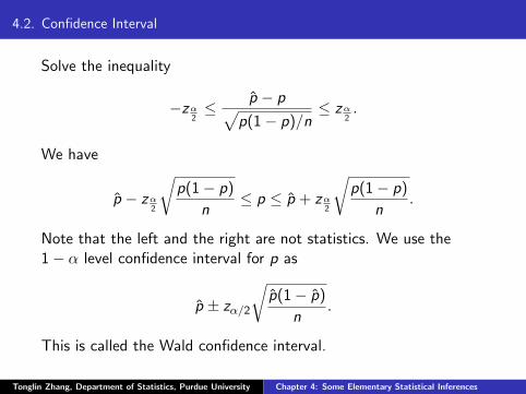
Solve the inequality
−zα2≤ p − p√
p(1− p)/n≤ zα
2.
We have
p − zα2
√p(1− p)
n≤ p ≤ p + zα
2
√p(1− p)
n.
Note that the left and the right are not statistics. We use the1− α level confidence interval for p as
p ± zα/2
√p(1− p)
n.
This is called the Wald confidence interval.
Tonglin Zhang, Department of Statistics, Purdue University Chapter 4: Some Elementary Statistical Inferences

4.2. Confidence Interval
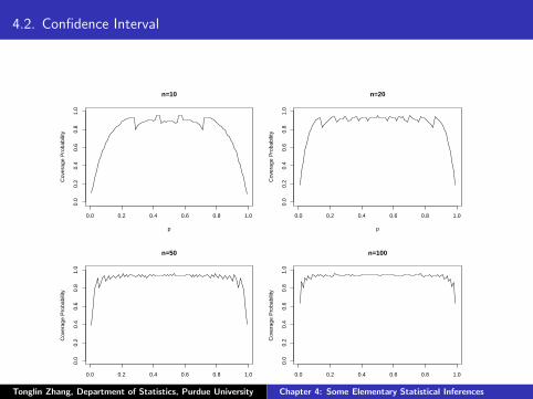
I also calculate the covarage probability of the Wald confidenceinterval by simulations. The result is displayed in Figure 2. Sincethe curve is not alway close to 0.95. The formulation may not becorrect.
Tonglin Zhang, Department of Statistics, Purdue University Chapter 4: Some Elementary Statistical Inferences
4.2. Confidence Interval
0.0 0.2 0.4 0.6 0.8 1.0
0.0
0.2
0.4
0.6
0.8
1.0
n=10
p
Cov
erag
e P
roba
bilit
y
0.0 0.2 0.4 0.6 0.8 1.0
0.0
0.2
0.4
0.6
0.8
1.0
n=20
p
Cov
erag
e P
roba
bilit
y
0.0 0.2 0.4 0.6 0.8 1.0
0.0
0.2
0.4
0.6
0.8
1.0
n=50
p
Cov
erag
e P
roba
bilit
y
0.0 0.2 0.4 0.6 0.8 1.0
0.0
0.2
0.4
0.6
0.8
1.0
n=100
p
Cov
erag
e P
roba
bilit
y
Figure : Coverage probability of the t-confidence intervals as functions ofµ when n = 10 and σ2 = 1.
Tonglin Zhang, Department of Statistics, Purdue University Chapter 4: Some Elementary Statistical Inferences
4.2. Confidence Interval
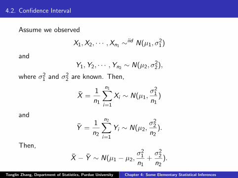
Assume we observed
X1,X2, · · · ,Xn1 ∼iid N(µ1, σ21)
andY1,Y2, · · · ,Yn2 ∼ N(µ2, σ
22),
where σ21 and σ2
2 are known. Then,
X =1
n1
n1∑i=1
Xi ∼ N(µ1,σ21
n1)
and
Y =1
n2
n2∑i=1
Yi ∼ N(µ2,σ22
n2).
Then,
X − Y ∼ N(µ1 − µ2,σ21
n1+
σ22
n2).
Tonglin Zhang, Department of Statistics, Purdue University Chapter 4: Some Elementary Statistical Inferences

4.2. Confidence Interval
Suppose that σ21 and σ2
2 are known. Write x and y are observedvalues of X and Y respectively. Then, the (1− α)100% confidenceinterval for µ1 − µ2 is
(X − y)± zα2
√σ21
n1+
σ22
n2.
Tonglin Zhang, Department of Statistics, Purdue University Chapter 4: Some Elementary Statistical Inferences
4.2. Confidence Interval
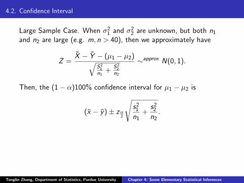
Large Sample Case. When σ21 and σ2
2 are unknown, but both n1and n2 are large (e.g. m, n > 40), then we approximately have
Z =X − Y − (µ1 − µ2)√
S21
n1+
S22
n2
∼approx N(0, 1).
Then, the (1− α)100% confidence interval for µ1 − µ2 is
(x − y)± zα2
√s21n1
+s22n2
.
Tonglin Zhang, Department of Statistics, Purdue University Chapter 4: Some Elementary Statistical Inferences

4.2. Confidence Interval
Pooled t-confidence interval. Assume σ21 = σ2
2. Let
S2p =
(n1 − 1)S21 + (n2 − 1)S2
2
n1 + n2 − 2
and write s2p as the observed value of S2p . Then,
T =X − Y − (µ1 − µ2)√
S2p (1/n1 + 1/n2)
∼ tn1+n2−2.
Thus, the (1− α)100% confidence interval for µ1 − µ2 is
x − y ± tα2,n1+n2−2sp
√1
n1+
1
n2.
Tonglin Zhang, Department of Statistics, Purdue University Chapter 4: Some Elementary Statistical Inferences
4.2. Confidence Interval
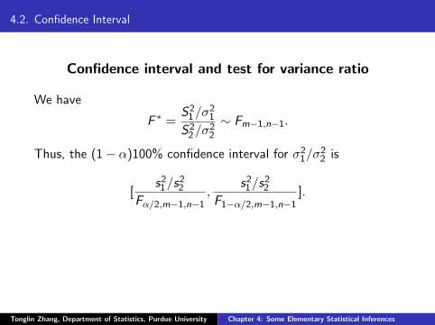
Confidence interval and test for variance ratio
We have
F ∗ =S21/σ
21
S22/σ
22
∼ Fm−1,n−1.
Thus, the (1− α)100% confidence interval for σ21/σ
22 is
[s21/s
22
Fα/2,m−1,n−1,
s21/s22
F1−α/2,m−1,n−1].
Tonglin Zhang, Department of Statistics, Purdue University Chapter 4: Some Elementary Statistical Inferences
4.2. Confidence Interval
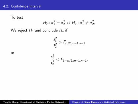
To testH0 : σ
21 = σ2
2 ↔ Ha : σ21 = σ2
2,
We reject H0 and conclude Ha if
s21s22
> Fα/2,m−1,n−1
ors21s22
< F1−α/2,m−1,n−1.
Tonglin Zhang, Department of Statistics, Purdue University Chapter 4: Some Elementary Statistical Inferences
4.2. Confidence Interval
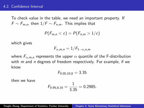
To check value in the table, we need an important property. IfF ∼ Fm,n, then 1/F ∼ Fn,m. This implies that
P(Fm,n < c) = P(Fn,m > 1/c)
which givesFα,m,n = 1/F1−α,n,m
where Fα,m,n represents the upper α quantile of the F-distributionwith m and n degrees of freedom respectively. For example, if weknow
F0.05,10,8 = 3.35
then we have
F0.95,8,10 =1
3.35= 0.2985.
Tonglin Zhang, Department of Statistics, Purdue University Chapter 4: Some Elementary Statistical Inferences

4.2. Confidence Interval
Assume, we have data
X ∼ Bin(n1, p1)
andY ∼ Bin(n2, p2),
and X and Y are independent. Let p1 = X/m and p2 = Y /n.Then,
p1 − p2 ∼approx N(p1 − p2,p1(1− p1)
n1+
p2(1− p2)
n2).
Tonglin Zhang, Department of Statistics, Purdue University Chapter 4: Some Elementary Statistical Inferences

4.2. Confidence Interval
Since we can estimate the variance
p1(1− p1)
n1+
p2(1− p2)
n2
byp1(1− p1)
n1+
p2(1− p2)
n2,
the large-sample (1− α)100% confidence interval for p1 − p2 is
p1 − p2 ± zα/2
√p1(1− p1)
n1+
p2(1− p2)
n2.
Tonglin Zhang, Department of Statistics, Purdue University Chapter 4: Some Elementary Statistical Inferences
4.4. Order Statistics
4.4. Order Statistics
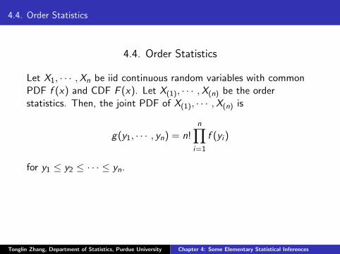
Let X1, · · · ,Xn be iid continuous random variables with commonPDF f (x) and CDF F (x). Let X(1), · · · ,X(n) be the orderstatistics. Then, the joint PDF of X(1), · · · ,X(n) is
g(y1, · · · , yn) = n!n∏
i=1
f (yi )
for y1 ≤ y2 ≤ · · · ≤ yn.
Tonglin Zhang, Department of Statistics, Purdue University Chapter 4: Some Elementary Statistical Inferences

4.4. Order Statistics
The marginal PDF of X(i) is
gi (yi ) =n!
(k − 1)!(n − k)![F (yi )]
i−1[1− F (yi )]n−i f (yi ).
The marginal PDF of X(i) and X(j) with i < j is
gij(yi , yj) =n!
(i − 1)!(j − i − 1)!(n − j)![F (yi )]
i−1
[F (yj)− F (yi )]j−i−1[1− F (yj)]
n−j f (yi )f (yj)
if yi ≤ yj .
Tonglin Zhang, Department of Statistics, Purdue University Chapter 4: Some Elementary Statistical Inferences
4.4. Order Statistics
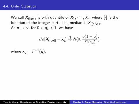
We call X([qn]) is q-th quantile of X1, · · · ,Xn, where [·] is thefunction of the integer part. The median is X([n/2]).As n → ∞ for 0 < q1 < 1, we have
√n[X([qn]) − xq]
D→ N(0,q(1− q)
f 2(xq)),
where xq = F−1(q).
Tonglin Zhang, Department of Statistics, Purdue University Chapter 4: Some Elementary Statistical Inferences
4.4. Order Statistics
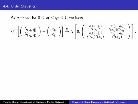
As n → ∞, for 0 < q1 < q2 < 1, we have
√n
[(X([q1n])
X([q2n])
)−(
xq1xq2
)]D→ N
0, q1(1−q1)
f 2(xq1 )q1(1−q2)
f (xq1 )f (xq2 )q1(1−q2)
f (xq1 )f (xq2 )q2(1−q2)f 2(xq2 )
.
Tonglin Zhang, Department of Statistics, Purdue University Chapter 4: Some Elementary Statistical Inferences
4.4. Order Statistics
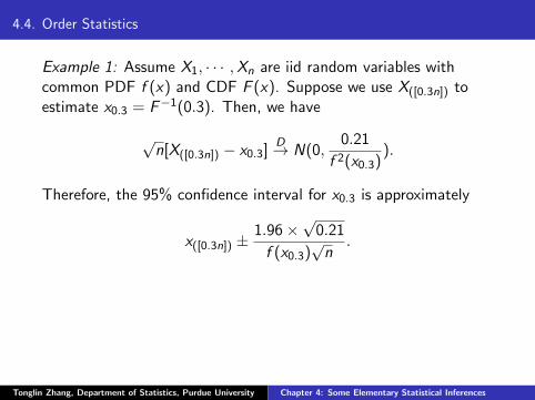
Example 1: Assume X1, · · · ,Xn are iid random variables withcommon PDF f (x) and CDF F (x). Suppose we use X([0.3n]) toestimate x0.3 = F−1(0.3). Then, we have
√n[X([0.3n]) − x0.3]
D→ N(0,0.21
f 2(x0.3)).
Therefore, the 95% confidence interval for x0.3 is approximately
x([0.3n]) ±1.96×
√0.21
f (x0.3)√n
.
Tonglin Zhang, Department of Statistics, Purdue University Chapter 4: Some Elementary Statistical Inferences
4.4. Order Statistics
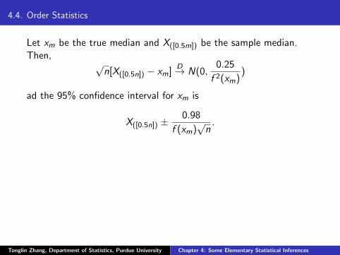
Let xm be the true median and X([0.5m]) be the sample median.Then,
√n[X([0.5n]) − xm]
D→ N(0,0.25
f 2(xm))
ad the 95% confidence interval for xm is
X([0.5n]) ±0.98
f (xm)√n.
Tonglin Zhang, Department of Statistics, Purdue University Chapter 4: Some Elementary Statistical Inferences

4.4. Order Statistics
Example 2: In the previous example, suppose
f (x) =1
π[1 + (x − θ)2],−∞ < x < ∞.
Then, θ is the median and θ = X([0.5n]) is an estimator of θ. Theconfidence interval for θ is
X([0.5n]) ±0.98π√
n.
Tonglin Zhang, Department of Statistics, Purdue University Chapter 4: Some Elementary Statistical Inferences
4.5 Introduction to Hypotheses Testing
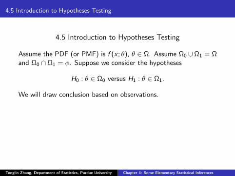
4.5 Introduction to Hypotheses Testing
Assume the PDF (or PMF) is f (x ; θ), θ ∈ Ω. Assume Ω0 ∪Ω1 = Ωand Ω0 ∩ Ω1 = ϕ. Suppose we consider the hypotheses
H0 : θ ∈ Ω0 versus H1 : θ ∈ Ω1.
We will draw conclusion based on observations.
Tonglin Zhang, Department of Statistics, Purdue University Chapter 4: Some Elementary Statistical Inferences
4.5 Introduction to Hypotheses Testing
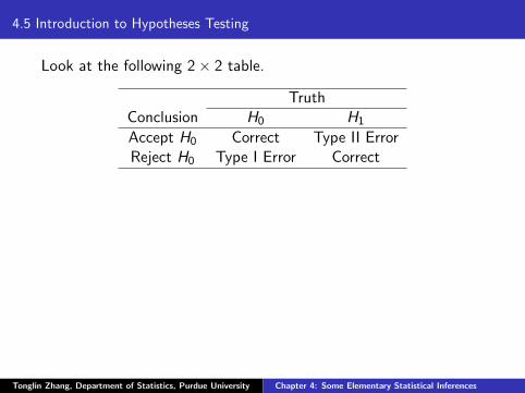
Look at the following 2× 2 table.
TruthConclusion H0 H1
Accept H0 Correct Type II ErrorReject H0 Type I Error Correct
Tonglin Zhang, Department of Statistics, Purdue University Chapter 4: Some Elementary Statistical Inferences
4.5 Introduction to Hypotheses Testing
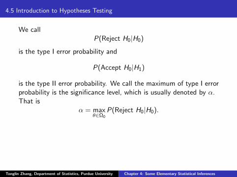
We callP(Reject H0|H0)
is the type I error probability and
P(Accept H0|H1)
is the type II error probability. We call the maximum of type I errorprobability is the significance level, which is usually denoted by α.That is
α = maxθ∈Ω0
P(Reject H0|H0).
Tonglin Zhang, Department of Statistics, Purdue University Chapter 4: Some Elementary Statistical Inferences
4.5 Introduction to Hypotheses Testing
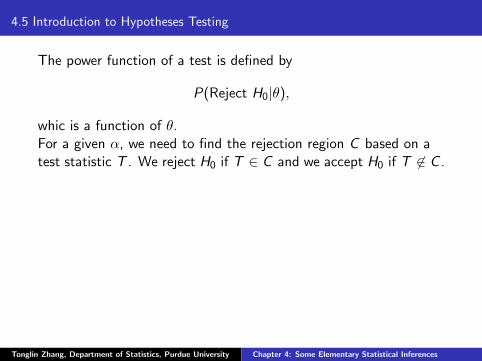
The power function of a test is defined by
P(Reject H0|θ),
whic is a function of θ.For a given α, we need to find the rejection region C based on atest statistic T . We reject H0 if T ∈ C and we accept H0 if T ∈ C .
Tonglin Zhang, Department of Statistics, Purdue University Chapter 4: Some Elementary Statistical Inferences

4.5 Introduction to Hypotheses Testing
Example: Suppose X1, · · · ,Xn are iid N(µ, 1). Let µ0 be a givennumber. We can test
(a) : H0 : µ ≤ µ0 ↔ H1 : µ > µ0
or(b) : H0 : µ ≥ µ0 ↔ H1 < µ0.
or(c) : H0 : µ = µ0 ↔ H0 = µ0.
Tonglin Zhang, Department of Statistics, Purdue University Chapter 4: Some Elementary Statistical Inferences
4.5 Introduction to Hypotheses Testing
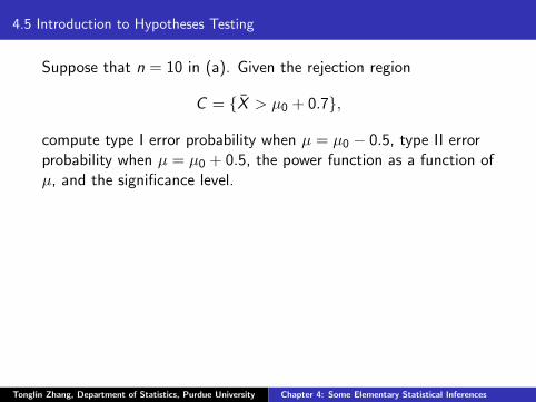
Suppose that n = 10 in (a). Given the rejection region
C = X > µ0 + 0.7,
compute type I error probability when µ = µ0 − 0.5, type II errorprobability when µ = µ0 + 0.5, the power function as a function ofµ, and the significance level.
Tonglin Zhang, Department of Statistics, Purdue University Chapter 4: Some Elementary Statistical Inferences

4.5 Introduction to Hypotheses Testing
Solution: Note thatX ∼ N(µ, 1/10).
The type I error probability when µ = µ− 0.5 is
P(Type I|µ = µ0 − 0.5) =P(Conclude µ > µ0|µ = µ0 − 0.5)
=P(X > µ0 + 0.7|µ = µ0 − 0.5)
=1− Φ(µ0 + 0.7− (µ0 − 0.5)√
1/10)
=1− Φ(1.2√1/10
)
=1− Φ(3.79)
=7.53× 10⁻⁵.
Tonglin Zhang, Department of Statistics, Purdue University Chapter 4: Some Elementary Statistical Inferences

4.5 Introduction to Hypotheses Testing
The type II error probability when µ = µ+ 0.5 is
P(Type II|µ = µ0 + 0.5) =P(Conclude µ ≤ µ0|µ = µ0 + 0.5)
=P(X ≤ µ0 + 0.7|µ = µ0 + 0.5)
=Φ(µ0 + 0.7− (µ0 + 0.5)√
1/10)
=Φ(0.2√1/10
)
=Φ(0.63)
=0.7356.
Tonglin Zhang, Department of Statistics, Purdue University Chapter 4: Some Elementary Statistical Inferences
4.5 Introduction to Hypotheses Testing
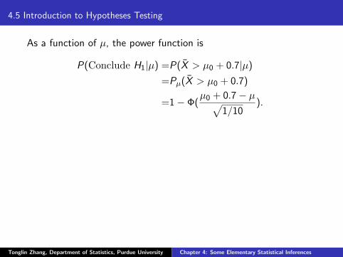
As a function of µ, the power function is
P(Conclude H1|µ) =P(X > µ0 + 0.7|µ)=Pµ(X > µ0 + 0.7)
=1− Φ(µ0 + 0.7− µ√
1/10).
Tonglin Zhang, Department of Statistics, Purdue University Chapter 4: Some Elementary Statistical Inferences
4.5 Introduction to Hypotheses Testing
−1 0 1 2 3
0.0
0.2
0.4
0.6
0.8
1.0
µ
Pow
er F
unct
ion
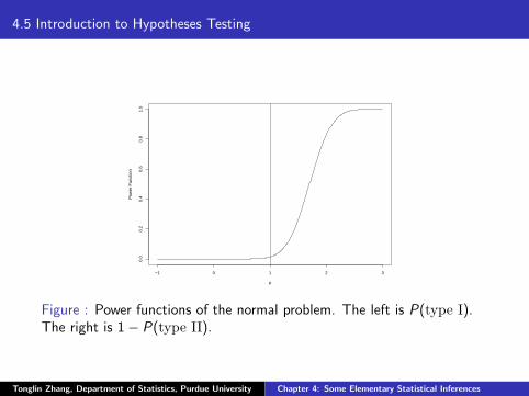
Figure : Power functions of the normal problem. The left is P(type I).The right is 1− P(type II).
Tonglin Zhang, Department of Statistics, Purdue University Chapter 4: Some Elementary Statistical Inferences

4.5 Introduction to Hypotheses Testing
The siginficance level is
α =maxH0
P(Type I)
=P(Type I|µ = µ0)
=1− Φ(0.7/√
1/10)
=1− Φ(2.21)
=0.0135.
Tonglin Zhang, Department of Statistics, Purdue University Chapter 4: Some Elementary Statistical Inferences
4.5 Introduction to Hypotheses Testing
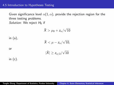
Given significance level α(1, α), provide the rejection region for thethree testing problems.Solution: We reject H0 if
X > µ0 + zα/√10
in (a),X < µ− zα/
√10,
or|X | ≥ zα/2/
√10
in (c).
Tonglin Zhang, Department of Statistics, Purdue University Chapter 4: Some Elementary Statistical Inferences
4.5 Introduction to Hypotheses Testing
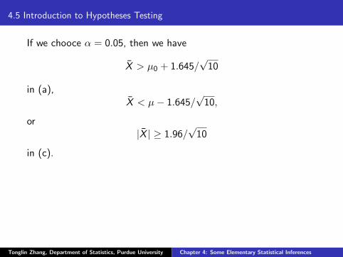
If we chooce α = 0.05, then we have
X > µ0 + 1.645/√10
in (a),X < µ− 1.645/
√10,
or|X | ≥ 1.96/
√10
in (c).
Tonglin Zhang, Department of Statistics, Purdue University Chapter 4: Some Elementary Statistical Inferences
4.5 Introduction to Hypotheses Testing
Example: Suppose X ∼ Bin(n, p). We can test
(a) H0 : p ≤ p0 ↔ H1 : p > p0
or(b) H0 : p ≥ p0 ↔ H1 : p < p0
or(c) H0 : p = p0 ↔ H1 : p = p0.
Suppose that n = 30 in (a) and p0 = 0.5. Given the rejectionregion
C = X ≥ 19,
compute type I error probability when µ = 0.3, type II errorprobability when µ = 0.7, the power function as a function of µ,and the significance level.
Tonglin Zhang, Department of Statistics, Purdue University Chapter 4: Some Elementary Statistical Inferences

4.5 Introduction to Hypotheses Testing
Solution: Note that X ∼ Bin(n, p). We have
P(Type I|p = 0.3) =P(X ≥ 19|p = 0.3)
=P(Bin(30, 0.3) ≥ 19)
=1.62× 10⁻⁴
andP(Type II|p = 0.7) =P(X < 19|p = 0.7)
=P(Bin(30, 0.7) ≤ 18)
=0.1593.
As a function of p, the power function is
P(Conclude H1|p) =P(X ≥ 19|p)=P(Bin(30, p) ≥ 19).
Tonglin Zhang, Department of Statistics, Purdue University Chapter 4: Some Elementary Statistical Inferences
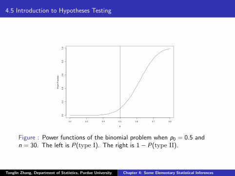
4.5 Introduction to Hypotheses Testing
0.2 0.3 0.4 0.5 0.6 0.7 0.8
0.0
0.2
0.4
0.6
0.8
1.0
p
Pow
er F
unct
ion
Figure : Power functions of the binomial problem when p0 = 0.5 andn = 30. The left is P(type I). The right is 1− P(type II).
Tonglin Zhang, Department of Statistics, Purdue University Chapter 4: Some Elementary Statistical Inferences

4.5 Introduction to Hypotheses Testing
Given significance level α ∈ (0, 1), provide the rejection region bythe Wald method.Solution: Let
Z =X − np0√np0(1− p0)
.
We call Z the test statistic. We reject H0 if
Z > zα
in (a). We reject H0 ifZ < −zα
in (b). We reject H0 if|Z | > zα/2
in (c).
Tonglin Zhang, Department of Statistics, Purdue University Chapter 4: Some Elementary Statistical Inferences
4.6 Additional Comments About Statistical Tests
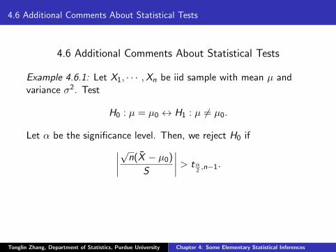
4.6 Additional Comments About Statistical Tests
Example 4.6.1: Let X1, · · · ,Xn be iid sample with mean µ andvariance σ2. Test
H0 : µ = µ0 ↔ H1 : µ = µ0.
Let α be the significance level. Then, we reject H0 if∣∣∣∣√n(X − µ0)
S
∣∣∣∣ > tα2,n−1.
Tonglin Zhang, Department of Statistics, Purdue University Chapter 4: Some Elementary Statistical Inferences

4.6 Additional Comments About Statistical Tests
Example 4.6.2: Assume X1, · · · ,Xn1 are iid N(µ1, σ2) and
Y1, · · · ,Yn2 are iid N(µ2, σ2). Test
H0 : µ1 = µ2 ↔ H1 : µ1 = µ2.
Suppose n is large. We reject H0 if∣∣∣∣∣∣ X − Y√S21/n1 + S2
2/n2
∣∣∣∣∣∣ > zα2.
Suppose that n is small but we assume σ21 = σ2
2 = σ2. Let
S2p =
(n1 − 1)S21 + (n2 − 1)S2
2
(n1 + n2 − 2).
We reject H0 is ∣∣∣∣∣ X − Y
Sp√
1/n1 + 1/n2
∣∣∣∣∣ > tα2,n1+n2−2.
Tonglin Zhang, Department of Statistics, Purdue University Chapter 4: Some Elementary Statistical Inferences
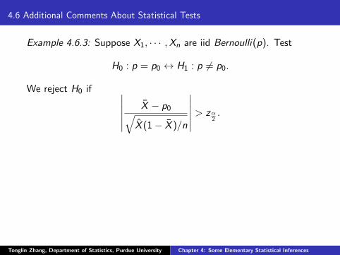
4.6 Additional Comments About Statistical Tests
Example 4.6.3: Suppose X1, · · · ,Xn are iid Bernoulli(p). Test
H0 : p = p0 ↔ H1 : p = p0.
We reject H0 if ∣∣∣∣∣∣ X − p0√X (1− X )/n
∣∣∣∣∣∣ > zα2.
Tonglin Zhang, Department of Statistics, Purdue University Chapter 4: Some Elementary Statistical Inferences
4.6 Additional Comments About Statistical Tests
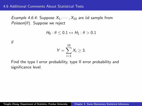
Example 4.6.4: Suppose X1, · · · ,X10 are iid sample fromPoisson(θ). Suppose we reject
H0 : θ ≤ 0.1 ↔ H1 : θ > 0.1
if
Y =10∑i=1
Xi ≥ 3.
Find the type I error probability, type II error probability andsignificance level.
Tonglin Zhang, Department of Statistics, Purdue University Chapter 4: Some Elementary Statistical Inferences
4.6 Additional Comments About Statistical Tests
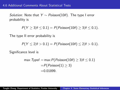
Solution: Note that Y ∼ Poisson(10θ). The type I errorprobability is
P(Y ≥ 3|θ ≤ 0.1) = P(Poisson(10θ) ≥ 3|θ ≤ 0.1).
The type II error probability is
P(Y ≤ 2|θ > 0.1) = P(Poisson(10θ) ≤ 2|θ > 0.1).
Significance level is
maxTypeI =maxP(Poisson(10θ) ≥ 3|θ ≤ 0.1)
=P(Poisson(1) ≥ 3)
=0.01899.
Tonglin Zhang, Department of Statistics, Purdue University Chapter 4: Some Elementary Statistical Inferences

4.6 Additional Comments About Statistical Tests
Example 4.6.5: Let X1, · · · ,X25 be iid sample from N(µ, 4).Consider the test
H0 : µ ≥ 77 ↔ H1 : µ < 77.
Then, we reject H0 is
X − 77√4/25
≤ −zα.
Suppose we observe x = 76.1. The p-value is
Pµ=77(X ≤ 76.1) = Φ(76.1− 77√
4/25) = Φ(−2.25) = 0.012.
Tonglin Zhang, Department of Statistics, Purdue University Chapter 4: Some Elementary Statistical Inferences
4.7 Chi-Square Tests
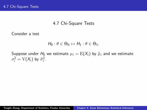
4.7 Chi-Square Tests
Consider a test
H0 : θ ∈ Θ0 ↔ H1 : θ ∈ Θ1.
Suppose under H0 we estimate µi = E(Xi ) by µi and we estimateσ2i = V(Xi ) by σ2
i .
Tonglin Zhang, Department of Statistics, Purdue University Chapter 4: Some Elementary Statistical Inferences

4.7 Chi-Square Tests
Pearson χ2 statistic. The Pearson χ2 statistic for independentrandom samples is
Y =n∑
i=1
(Xi − µi )2√
σ2i
.
The idea is motivated from independent normal distributions.Assume that X1, · · · ,Xn are independent N(µi , σ
2i ), respectively.
Then,
X 2 =n∑
i=1
(Xi − µi )2
σ2i
∼ χ2n.
Tonglin Zhang, Department of Statistics, Purdue University Chapter 4: Some Elementary Statistical Inferences

4.7 Chi-Square Tests
Loglikelihood ratio statistic. Let ℓ(θ) be the likelihood function.Then, the loglikelihood ratio statistic is defined by
Λ = 2 logsupθ∈Θ ℓ(θ)
supθ∈Θ0ℓ(θ)
= 2[log supθ∈Θ
ℓ(θ)− supθ∈Θ0
ℓ(θ)].
Tonglin Zhang, Department of Statistics, Purdue University Chapter 4: Some Elementary Statistical Inferences
4.7 Chi-Square Tests
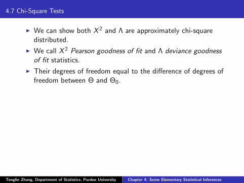
I We can show both X 2 and Λ are approximately chi-squaredistributed.
I We call X 2 Pearson goodness of fit and Λ deviance goodnessof fit statistics.
I Their degrees of freedom equal to the difference of degrees offreedom between Θ and Θ0.
Tonglin Zhang, Department of Statistics, Purdue University Chapter 4: Some Elementary Statistical Inferences
4.7 Chi-Square Tests
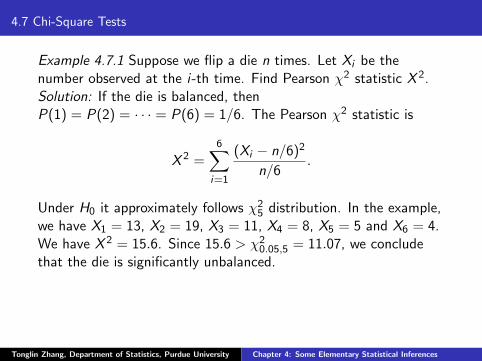
Example 4.7.1 Suppose we flip a die n times. Let Xi be thenumber observed at the i-th time. Find Pearson χ2 statistic X 2.Solution: If the die is balanced, thenP(1) = P(2) = · · · = P(6) = 1/6. The Pearson χ2 statistic is
X 2 =6∑
i=1
(Xi − n/6)2
n/6.
Under H0 it approximately follows χ25 distribution. In the example,
we have X1 = 13, X2 = 19, X3 = 11, X4 = 8, X5 = 5 and X6 = 4.We have X 2 = 15.6. Since 15.6 > χ2
0.05,5 = 11.07, we concludethat the die is significantly unbalanced.
Tonglin Zhang, Department of Statistics, Purdue University Chapter 4: Some Elementary Statistical Inferences
4.7 Chi-Square Tests
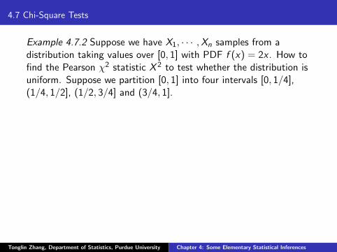
Example 4.7.2 Suppose we have X1, · · · ,Xn samples from adistribution taking values over [0, 1] with PDF f (x) = 2x . How tofind the Pearson χ2 statistic X 2 to test whether the distribution isuniform. Suppose we partition [0, 1] into four intervals [0, 1/4],(1/4, 1/2], (1/2, 3/4] and (3/4, 1].
Tonglin Zhang, Department of Statistics, Purdue University Chapter 4: Some Elementary Statistical Inferences
4.7 Chi-Square Tests
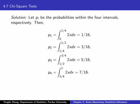
Solution: Let pi be the probabilities within the four intervals,respectively. Then,
p1 =
∫ 1/4
02xdx = 1/16,
p2 =
∫ 1/2
1/42xdx = 3/16,
p3 =
∫ 3/4
1/22xdx = 5/16,
p4 =
∫ 1
3/42xdx = 7/16.
Tonglin Zhang, Department of Statistics, Purdue University Chapter 4: Some Elementary Statistical Inferences

4.7 Chi-Square Tests
Let ni be the total counts in the intervals, respectively. Then,
X 2 =(n1 − n/16)2
n/16+(n2 − 3n/16)2
3n/16+(n3 − 5n/16)2
5n/16+(n4 − 7n/16)2
7n/16.
If the true distribution is the given distribution, then X 2 ∼ χ23
approximately. Based on data n1 = 6, n2 = 18, n3 = 20, andn4 = 36. We obtain X 2 = 1.83. Since it is less than χ2
0.05,3 = 7.81,we conclude that the true distribution is not significantly differentfrom the given distribution.
Tonglin Zhang, Department of Statistics, Purdue University Chapter 4: Some Elementary Statistical Inferences