Chapter 4: Small Commercial and Residential Unitary and Split System HVAC Cooling Equipment-Efficiency Upgrade Evaluation Protocol

David Jacobson, Jacobson Energy Research Subcontract Report NREL/SR-7A30-53827 April 2013

4 - 1

Chapter 4 – Table of Contents 1 Measure Description .............................................................................................................. 2 2 Application Conditions of Protocol ....................................................................................... 3

2.1 Programs with Enhanced Measures ................................................................................. 5 3 Savings Calculations .............................................................................................................. 6 4 Measurement and Verification Plan ....................................................................................... 8

4.1 IPMVP Option ................................................................................................................. 8 4.2 Secondary Options ......................................................................................................... 10 4.3 Verification Process ....................................................................................................... 11 4.4 Data Requirements ......................................................................................................... 12 4.5 Data Collection Methods ............................................................................................... 12

5 Sample Design ..................................................................................................................... 16 6 Program Evaluation Elements.............................................................................................. 17

6.1 Net-to-Gross ................................................................................................................... 17 7 References ............................................................................................................................ 18 8 Resources ............................................................................................................................. 20

4 - 2

1 Measure Description A packaged system—often called a “rooftop unit” because it is usually installed on the roof of a small commercial building—puts all cooling and ventilation system components (evaporator, compressor, condenser, and air handler) in one enclosure or package. The capacity of packaged systems typically ranges from 3 to 20 tons, although a system can be more than 100 tons.

Split systems primarily are used for residences and very small commercial spaces. These systems place condensers and compressors outdoors and place evaporators and supply fans indoors. On average, split systems have a capacity of less than 65,000 Btu/hr (5.4 tons).1 Small systems are rated using the Air-Conditioning, Heating, and Refrigeration Institute (AHRI) standard 210/240, while the large systems are rated using AHRI 340/360.

1 A ton equals 12,000 Btu/hr, or the amount of power required to melt 1 ton of ice in 24 hours.

4 - 3

2 Application Conditions of Protocol The specific measure described here involves improving the overall efficiency in air-conditioning systems as a whole (compressor, evaporator, condenser, and supply fan). The efficiency rating is expressed as the energy efficiency ratio (EER), seasonal energy efficiency ratio (SEER), and integrated energy efficiency ratio (IEER). The higher the EER, SEER or IEER, the more efficient the unit is.

• EER is the Btu/hr of peak cooling delivered per watt of electricity used to produce that amount of cooling. Generally, the EER is measured at standard conditions (95oF outdoor dry bulb, 67oF indoor wet bulb), as determined by the AHRI Standard 210/240 (AHRI 2008).

• SEER is a measure of a cooling system’s efficiency during the entire cooling season for units of less than 65,000 Btu/hr (less than 5.4 tons). The SEER, determined at part load, is measured at average conditions (82oF), as established by AHRI 210/240-2008.

• IEER is a measure of a cooling system’s efficiency during the entire cooling season for units of 65,000 Btu/hr (5.4 tons) and more, expressed in Btu/hr of cooling per watt of electric input. AHRI Standard 340/360 2007 defines IEER as “a single number figure of merit expressing cooling part-load EER for commercial unitary air-conditioning equipment and heat pump equipment on the basis of weighted operation at various load capacities.” It replaces the Integrated Part Load Performance (IPLV) in AHSRAE standard 90.1-2007.

For many commercial unitary rebate programs offered in 2011 and 2012, units greater than 5.4 tons are qualified based on the EER only, and IEER is not captured. Although IEER provides a more accurate measure of seasonal efficiency for larger units, it is not yet commonplace throughout the incentive program community.

Table 1 presents a typical program offering for this measure.2

2 MassSave Cool Choice Program, offered in 2012 by all Massachusetts Program Administrators. See

www.masssave.com/~/media/Files/Professional/Applications-and-Rebate-Forms/Cool_Choice_MA_Form_fnl.ashx.

4 - 4

Table 1: Typical Incentive Offering for Air-Cooled Unitary AC and Split Systems (New Condenser and New Coil)

This measure’s primary delivery channel is a rebate program, usually marketed through program administrator staffs and heating, ventilating, and air-conditioning (HVAC) contractor partners. Typically, these programs do not include early replacement incentives, except when unusually high use of air-conditioning occurs.

• Rebates for units installed in commercial settings are typically paid on the basis of dollars-per-ton of cooling, which can vary by the efficiency level achieved (CEE 2009).

• Rebates for residential units are often paid on a fixed rebate-per-unit basis to discourage oversizing and to promote high-quality installation practices.

The rebates apply (1) at the time of normal replacement due to age or failure or (2) for new construction applications.

When a unit is installed in new construction or replaces an existing unit that has failed or is near the end of its life, the baseline efficiency standard it must meet is generally defined by local energy codes, federal manufacturing standards, or ASHRAE Standard 90.1 for SEER-rated units (less than 5.4 tons) and IEER-rated units (5.4 tons or greater). This protocol assumes more efficient equipment of the same capacity runs the same number of hours as the baseline equipment. It does not cover:

• Early replacement retrofits

• Right-sizing initiatives

• Tune-ups

• Electronically commutated motors (ECM) retrofits on fans

• Savings resulting from installation of an economizer or demand controlled ventilation at the same time as installation of the new, high-efficiency equipment.

Tons Min. SEER/EER for Incentive

Incentive $/Ton

Min. SEER/EER for Incentive

Incentive $/Ton

< 5.4 < 65,000 Split14.0 SEER & 12.0 EER $70

15.0 SEER & 12.5 EER $125

< 5.4 < 65,000 Packaged14.0 SEER & 11.6 EER $70

15.0 SEER & 12.0 EER $125

≥ 5.4 to < 11.25 11.5 EER $50 12.0 EER $80 ≥ 11.25 to < 20 11.5 EER $50 12.0 EER $80

≥ 20 to < 63 10.5 EER $30 10.8 EER $50 ≥ 63 N/A N/A 10.2 EER $50

≥ 135,000 to < 240,000≥ 240,000 to < 760,000

≥ 760,000

Efficiency TierUnit SizeLevel 1 Level 2

Btuh 

≥ 65,000 to < 135,000

4 - 5

2.1 Programs with Enhanced Measures Many program administrators offer other cooling measures in conjunction with higher EER/SEER/IEER cooling units. These measures include dual enthalpy economizers, demand controlled ventilation, and ECMs for ventilation fans as a retrofit or an upgrade option at the time of replacement.

Other programs, particularly residential, also focus on high-quality installation by requiring the work to meet Air Conditioning Contractors of America (ACCA) Quality Installation (QI) standards, which encompass proper duct sealing (ACCA 2007).

The evaluation methods addressed in this protocol do not include—on a standalone basis—savings resulting from these other measures. However, some overlap may occur with the evaluation, measurement, and verification (EM&V) of high-efficiency cooling system upgrades, particularly with demand controlled ventilation, ECMs, and dual enthalpy economizers.

2.1.1 Economizers Economizers work by bringing in outside air for ventilation and cooling, when outside conditions are sufficiently cool. In some jurisdictions, many of the newer packaged or split systems have temperature or dry bulb-based economizers, as required by code or by standard practice. Units with temperature-based economizers can be included in samples as a random occurrence, reflected in approximately rough proportion to their penetration in the population.

A dual-enthalpy economizer—a more sophisticated type, controlling both temperature and humidity—brings in outside air when the outside conditions are sufficiently cool and dry. These units tend to reduce the run hours of high-efficiency air conditioners as compared to units without economizers, thus reducing potential savings from more efficient units. Although dual-enthalpy economizers usually are not required by code, some utilities provide an incentive for them. If programs offer additional incentives for dual-enthalpy economizers, savings for those measures should not be estimated using the protocol described here.

2.1.2 Demand Controlled Ventilation Demand controlled ventilation (which uses a CO2 sensor on return air to limit the intake of outside air to be cooled) can reduce the run hours for unitary and split systems. Units that receive rebates for demand controlled ventilation should not use this protocol, which assumes the operating hours remain constant.

2.1.3 Right-Sizing The savings estimated for this measure do not include the effects of right-sizing initiatives, which match outputs of cooling systems with cooling loads of facilities (thereby optimizing systems’ operations). The high-efficiency upgrade measure described here assumes both the base or code-compliant units and the high-efficiency units installed are the same size. Thus, the savings achieved through right-sizing initiatives must be determined using a more complex analysis method than is described here.

4 - 6

3 Savings Calculations The calculation of gross annual energy savings for this measure, as defined by a large number of technical reference manuals (TRMs) (Massachusetts Program Administrators 2011,United Illuminating Company and Connecticut Lighting and Power Company 2008, Vermont Energy Investment Corporation 2010), uses the following algorithms.

Equation 1 (for units with a capacity of 5.4 tons or more)

kWh Saved = (Size kBtu/hr) * (1/EERbaseline – 1/EERinstalled) * (EFLH)

Equation 2 (for units having a capacity of fewer than 5.4 tons)

kWh Saved = (Size kBtu/hr) * (1/SEERbaseline – 1/SEERinstalled) * (EFLH) where:

kWh Saved = kilowatt-hours saved Size kBtu/hr = cooling capacity of unit EERbaseline = energy efficiency ratio of the baseline unit, as defined by local code EERinstalled = energy efficiency ratio of the specific high-efficiency unit SEERbaseline = seasonal energy efficiency ratio of the baseline unit, as defined by local

code SEERinstalled = seasonal energy efficiency ratio of the specific high-efficiency unit EFLH = equivalent full-load hours for cooling

Although at this time, many efficiency providers use Equation 2 with EER for units of greater than 5.4 tons, the protocol recommends using the more accurate measure of seasonal efficiency, IEER, shown in Equation 3.

Equation 3 (for IEER)

kWh Saved = (Size kBtu/hr) * (1/IEERbaseline – 1/IEERinstalled) * (EFLH) where:

IEERbaseline = Integrated energy efficiency ratio of the baseline unit, defined to be minimally compliant with code, which is usually based on ASHRAE 90.1-2010

IEERinstalled = Integrated energy efficiency ratio of the specific high-efficiency unit Note that for many programs currently offered, only EER is required to qualify units 5.4 tons or greater. For smaller units, SEER is almost always available, and it should be used for the calculation of annual energy savings.

This formula assumes some simplifications: (1) baseline units and high-efficiency units are of equal size (that is, no downsizing or “rightsizing” due to increased efficiency); and (2) baseline

4 - 7

and high-efficiency units have the same operating hours. Although this may not be the case for a given cooling load, these simplifications have been determined reasonable in the context of other uncertainties.

4 - 8

4 Measurement and Verification Plan When choosing an option, consider the following factors:

• The equation variables used to calculate savings

• The uncertainty in the claimed estimates of each parameter

• The cost, complexity, and uncertainty in measuring each of those variables.

When calculating savings for unitary HVAC, the goal is to take unit measurements as cost-effectively as possible, so as to reduce overall uncertainty in the savings estimate. Thus, use these primary components:

• Unit size

• Efficiency of the base unit and the installed unit

• Annual operating hours for energy savings

• Coincidence factor (CF) for demand savings.

4.1 IPMVP Option The recommended approach entails two steps: (1) Use one of the equations provided above with manufacturer rated values for capacity and efficiency (using industry-approved methods); and (2) incorporate program-specific measured values for the operating hours. (This approach most closely resembles International Performance Measurement and Verification Protocol (IPMVP) Option A: Partial Retrofit Isolation/Metered Equipment.)

Option A can be considered the best approach for the following reasons:

• The key issue for replace-on-failure/new construction programs is the usage of baseline equipment, defined as the current code or prevailing standard. However, this cannot be measured or assessed for participating customers because, by definition, lower-efficiency baseline equipment was never installed. The unit replaced is often old and below current requirements and is not the appropriate baseline. A nonparticipant group installing baseline equipment could be used, but only one known study has attempted this to date (KEMA 2010). For most situations, finding valid nonparticipants through random-digit dialing and performing extensive metering is simply too costly, given the savings level this measure contributes to typical portfolios.3

• Regarding the use of pre/post-billing analysis (IMPVP Option C) for participants, the same issue applies—pre-installation does not represent the baseline. Even without using pre/post-billing analysis, one might try using monthly billing data to determine cooling energy for a facility and then calculate facility-level full-load hours for use in the equations. However, this method is not recommended because cooling electricity

3 This generally represents a small percentage of total commercial and industrial portfolio savings; primarily due

to code, most new equipment is already relatively efficient.

4 - 9

usage cannot be easily disaggregated from total monthly electric usage with the accuracy required. As more residential and small commercial customers get kilowatt (kW) interval data (hourly or smaller time intervals), estimating cooling hours from whole-building data may become more feasible for very simple cases, but such methods are error-prone; feasibility will depend strongly on building size and type, HVAC system configuration, and the profiles of other loads.

4.1.1 Capacity Measuring cooling capacity is extremely expensive and would only result in replicating information already provided in a manner overseen by a technical standards group (AHRI). Thus, for a unit’s peak cooling capacity (size), use the manufacturer’s ratings, as these have generally been determined through an industry-standard approved process at fixed operating conditions. Although some variation may occur in the output of individual rebated units, it is assumed that on average, units perform close to AHRI ratings.

4.1.2 Efficiency Rating For determining the efficiency levels of base units and installed units, an industry accepted standard alternative to in situ measurement is available through manufacturers’ ratings. (Also, performing in situ measuring is extremely costly.)

4.1.3 Equivalent Full-Load Hours The EFLH variable must be measured or estimated for the population of program participants. Operating hours are specific to building types and to system sizing and design practices. Typical design practice tends to result in oversizing (using a larger-than-needed unit). In general, the greater the oversizing, the fewer the operating hours, and the less efficiently a unit operates.

Two primary methods exist for developing hours of use for the equations in Savings Calculations—creating a building simulation or conducting metering. The recommended approach favors using some actual measurement rather than relying exclusively on simulation-based estimates.

Detailed building simulation models can be developed for a wide variety of building types, system configurations, and applicable weather data. Such analysis usually results in an extensive set of look-up tables for operating hours listed by building type and weather zone. Various TRMs use this approach, including New York and California (TecMarket Works 2010) (Itron, Inc. 2005). In California, DEER look-up tables contain 9,000 unique combinations of unit types, building vintages, climate zones, and building types.

This approach is used to establish program planning estimates when measurements are not available, but it does not include measurements to account for oversizing practices or the types of building populations served by the actual programs. Thus, the recommended approach entails metering demand (kW) for a sample of units to develop EFLH estimates (KEMA 2010).

Note that the energy consumption of the compressor(s), condenser fan(s), and evaporator (i.e. supply) fan(s) are used to calculate the EFLH, but only when the compressor and condenser actually supply cooling.

4 - 10

Measurement of energy consumption can be used to validate building simulation models. However, in practice, the cost of metering the sample sizes required for developing data for all building types and weather zones would be cost-prohibitive and thus has not been attempted. In a California study, results from approximately 50 units in three climate zones were used to develop realization rates to calibrate the simulation approach to metered data, but not to determine EFLH for combinations of building types, climate zones, and system types (Itron, Inc. and KEMA 2008).

Measuring energy consumption involves on-site inspections, where unit-level power metering is performed for a wide range of temperature, occupancy, and humidity conditions. The resulting data can be analyzed to determine energy consumption as a function of outdoor wet-bulb or dry-bulb temperatures. These data can be extrapolated to the entire year by using typical meteorological year (TMY) data.

Dividing annual energy consumption (kWh) by the peak rated kW serves as a proxy for EFLH. The peak rated kW is defined as a unit’s peak cooling capacity at AHRI conditions in kBtu/hr and divided by the EER. Metering used to determine the annual kWh consumption should be based on either (1) a true power (kW) meter and integration of power over time; or (2) an energy meter, which performs the integration internally. Such metering should include the compressor(s), condenser fan(s), and supply fan(s). If true power kW or energy metering proves too costly, amperage data may be acceptable if they are supplemented with spot power measurements under a variety of loading conditions.

When taking measurements, consider these factors: (1) Use a random sample of units spread across building types and (2) stratify the sample by climate zone (if the territory has a wide range of temperature and humidity conditions) and unit sizes. Note that unit-size stratification may not be required if unit sizes fall within a narrow range.

Although a sufficiently large random sample would likely capture the predominant building types of interest, we recommend checking distributions of building types in the sample relative to the population and then adjusting or redrawing the sample, as needed, if an adequate distribution does not result.

4.2 Secondary Options More extensive measurements than those described above may be justified when (1) typical operating conditions are significantly different than conditions for which the equipment has been rated or (2) the savings for this measure make up a significant portion of total portfolio savings. For example, extensive measurements may be appropriate in very hot and dry climates (such as the Southwest), where the dry-bulb temperature is often higher than the 95oF used for EER ratings and the humidity is very low, compared to conditions for SEER ratings. Navigant (Navigant 2010) has shown that performance in hot, dry climates differs significantly from manufacturers’ standard conditions.

Another complicating issue is performance at low loading for large units, with multiple compressors running in parallel. In such cases, low-loading performance is higher than expected from typical SEER ratings. If a part-load rating is available that matches operating conditions

4 - 11

reasonably well, use SEER or IEER in place of EER for simplified equations calculating energy savings in conjunction with metered estimates of full-load hours.

In cases such as these where more extensive measurement is justified, consider the following steps:

1. Meter equipment to determine runtimes in high and low stages of operation.

2. Aggregate and normalize runtime data for weather effects to create a typical hourly runtime shape that corresponds with a typical set of weather conditions.

3. Collect detailed performance data for a representative selection of equipment of various IEER/IPLV, EER, or SEER.

4. Calculate hourly kWh/ton using detailed performance data and runtimes for each hour for each piece of equipment.

5. Sum the hourly kWh/ton over the full year to calculate annual kWh/ton and then average hourly kWh/ton over the peak period to calculate peak kW/ton.

6. Fit a mathematical function to determine kWh/ton = f(SEER or IEER, EER) and kW/ton = f(SEER or IEER, EER).

7. Apply the mathematical functions for kWh/ton and kW/ton to the population’s energy-efficient and baseline cases to determine savings for each piece of equipment.

An alternative for jurisdictions with detailed TRMs (such as New York) is the option used by Itron and KEMA in California, which involved measurement for a sample of units and development of a relationship between metered EFLH and that predicted by simulation models (Itron, Inc. and KEMA 2008). Expressed as a realization rate, such a relationship can be used for all unmetered sites to adjust simulation-based EFLH values. This alternative approach, however, is very expensive and, for equivalent funding, using the recommended approach can result in obtaining measurement data from five to 10 times more pieces of equipment. (Other measurement options are discussed in various ASHRAE publications [ASHRAE 2000] [ASHRAE 2002] [ASHRAE 2010].)

If all detailed measurements fall beyond an evaluation’s available budget, program administrators can use available EFLH data from studies conducted for similar climate zones and building types. This approach, however, involves no actual measurements to reflect typical system sizing and design practices, building types, or weather in a region or service territory.4

4.3 Verification Process The key data to be verified are (1) the size of the unit rebated and (2) the efficiency of the installed unit. Verification can be performed through:

4 As discussed in the Considering Resource Constraints section of the “Introduction” chapter to this UMP report,

small utilities (as defined under the U.S. Small Business Administration [SBA] regulations) may face additional constraints in undertaking this protocol. Therefore, alternative methodologies should be considered for such utilities.

4 - 12

• A desk review of invoices and manufacturers’ specification sheets (which should be required for rebate payment)

• An on-site audit of a sample of participants (usually the same participants selected for the end-use metering, discussed above).

Cooling capacity and efficiency are measured by manufacturers under standard conditions; however, the EFLH is site-dependent and not measured. Thus, the major uncertainty arises in the EFLH, so metering should concentrate on that quantity.

If savings can be determined as a function of building types, then verification of building types on applications can be conducted through on-site visits or telephone surveys.

Baseline efficiency can be assumed to be that of a code-compliant unit in the service territory. Differences in efficiency between code-compliant units and standard practice would be reflected in the calculation of an appropriate net-to-gross ratio.

4.4 Data Requirements Minimum data required for evaluating a unitary HVAC rebate program are:

• Size (in Btu/hr or tons) of each unit installed

• Efficiency (in EER, SEER, or IEER) of each unit installed

• Assumed baseline efficiency for each category of units (from prevailing code or standard)

• Location of each unit, corresponding to specific weather station disaggregation used for analysis of metered data.

Metered data used in the evaluation consists of the EFLH developed for each weather zone, which is derived as the ratio of the annual kWh divided by the peak kW.

Using the appropriate equation in Savings Calculations, determine the savings for this measure with these data:

• The installed cooling capacity

• The EER, SEER, or IEER rating (from manufacturers’ data) of the baseline unit and the installed unit

• The measured EFLH.

4.5 Data Collection Methods Given the relative size of savings for this measure in a typical portfolio—one dominated by other higher-savings measures—the collection of data (which is comparatively costly) can best be conducted jointly with other program administrators in a state or region with similar weather conditions.

In the past 15 years, a number of studies have examined commercial unitary HVAC EFLH and load shapes of note (KEMA 2011) (SAIC 1998) (Itron, Inc. and KEMA 2008) (KEMA 2010).

4 - 13

Further, at least two studies have examined full-load hours of residential central air-conditioning systems (KEMA 2009) (ADM 2009). The method this protocol recommends has been based on work described in the Northeast Energy Efficiency Partnerships (NEEP) EM&V Forum study (KEMA 2011), which, if conducted on a regional basis across multiple program administrators, balances rigor and cost.

As discussed, unit sizes and climate zones provide variables for developing a sampling framework. Large units tend to run for more hours and exhibit higher peak coincidence than small units (ranging from 3 tons to 15 tons). Large units also tend to use multiple compressors and are controlled differently than smaller, single-compressor units.

If a program predominantly rebates units smaller than 15 tons in size (or if the specific prescriptive program is limited to units smaller than 15 tons), only one size category is necessary. Similarly, if all units in the service territory or region studied have essentially the same temperature and humidity conditions (for example, one large city), sampling by climate zone is not needed.

Thus, if unit size and climate zone are not required sampling dimensions for representing the population, then sampling by predominant building type alone may be possible. Otherwise, sampling by combinations of climate zone, size, and building type may prove impractical.

4.5.1 Metering Metering should capture integrated true root mean square (RMS) kW power measurements at 15 minute intervals during at least half of the typical cooling season for the region, being sure to include either the spring or fall shoulder periods. If budget allows, metering should extend from the time units typically come on in spring until units are no longer needed in fall. Where budgets are constrained and timing allowed is not sufficient, the evaluator may meter for less time but should assure that the monitoring captures the preponderance of operating conditions to minimize the extent to which extrapolation must be performed outside the range of conditions captured. For high internal gain situations where cooling is needed year round, metering should include some portion of the warmest weather and coldest weather months.

If the evaluation is also designed to capture oversizing practices of the newly installed units, more detailed cycling patterns beyond the determination of EFLH, and/or demand savings factors, data should be captured in 1-minute intervals (as data storage and budget constraints allow). Regardless of which metering intervals are used, data will be aggregated to one-hour averages for use in the model specified below because publicly-available weather data are generally available in hourly formats.

If budgets do not allow for measurement of kW using amperage and voltage measurements, using amperage measurements alone to determine EFLH and demand savings factors may be justified and is preferable over using values from studies conducted by other program administrators for similar climate zones and building types as described above. Direct kW measurements are preferable and the methods below assume kW measurements are taken. If amperage measurements are used, slight modifications to the formulas below for calculating EFLH are required.

4 - 14

The kW measurements should encompass the energy consumption of the compressor, condenser, evaporator, and supply fans. However, these measurements should only be used in the computation of the EFLH, when the compressor and condenser are actually running and supplying cooling. The accuracy of kW measurements should be ± 2%, as recommended by Independent System Operator (ISO) New England (ISO-New England, Inc. 2010).

After collecting the kW data, perform a unit-level regression of the unit power against predictor variables such as real-time weather data and whether the specific hour fell within the second or third hot day in a row. The predictor variables selected should provide the most significant independent variables for use as inputs to estimate the weather-normalized annual kWh consumption, and to extrapolate consumption outside the metering period. The result will be an 8760 kW load profile for that specific unit using the predictor variables. The following model functional form has been successfully used for this analysis in Northeast climates (KEMA 2011). Modifications to this model may be justified by the climate conditions and evaluation scope:5

(2)

Where, for a particular HVAC unit:

Ldh = load on day d hour h, day= 1 to 365, hour = 1 to 8760 in kW THIdh = temperature-humidity index on day d hour h w(d) = 0/1 dummy indicating day type of day d, Monday = 1, Sunday =7,

Holiday = 8 g(h) = 0/1 dummy indicating hour group for hour h, hour group = 1 to 24 H2d = 0/1 dummy indicating that hours in day d are the second hot day in a

row H3d = 0/1 dummy indicating that hours in day d are the third or more hot day

in a row α βCh βHh βw(d) βg(h) = coefficients determined by the regression β2h, β3h = hot day adjustments, a matrix of coefficients assigned to binary variables

(0/1) for hours defined for 2nd and 3rd consecutive hot days; matrix variables are unique to each hour in each hot day

εdh = residual error

The THI in °F can be defined as:

Where:

OSAdb = outside dry bulb temperature in °F DPT = outside air dew point temperature in °F

5 For example, in hotter climates, the variable for consecutive hot days may not be needed or, in more humid

climates, the dry bulb temperature and humidity may need to be separated

dhdhdhhgdwdhChdh HHhgdwTHIL εβββββα ++++++= 3322)()( )()(

153.05.0 +×+×= DPTOSATHI db

4 - 15

Note that this particular functional form is just an example of what has been successfully used. However, this protocol is not suggesting that using this specific regression model is a requirement. Other examples of modifications include using a variable for the presence of economizers or using log functions with independent variables. The success of the model should be measured by diagnostics such as signs for coefficients and comparison of measured power to modeled power via root mean squared error (RMSE), R-square for the model, and the mean bias error.

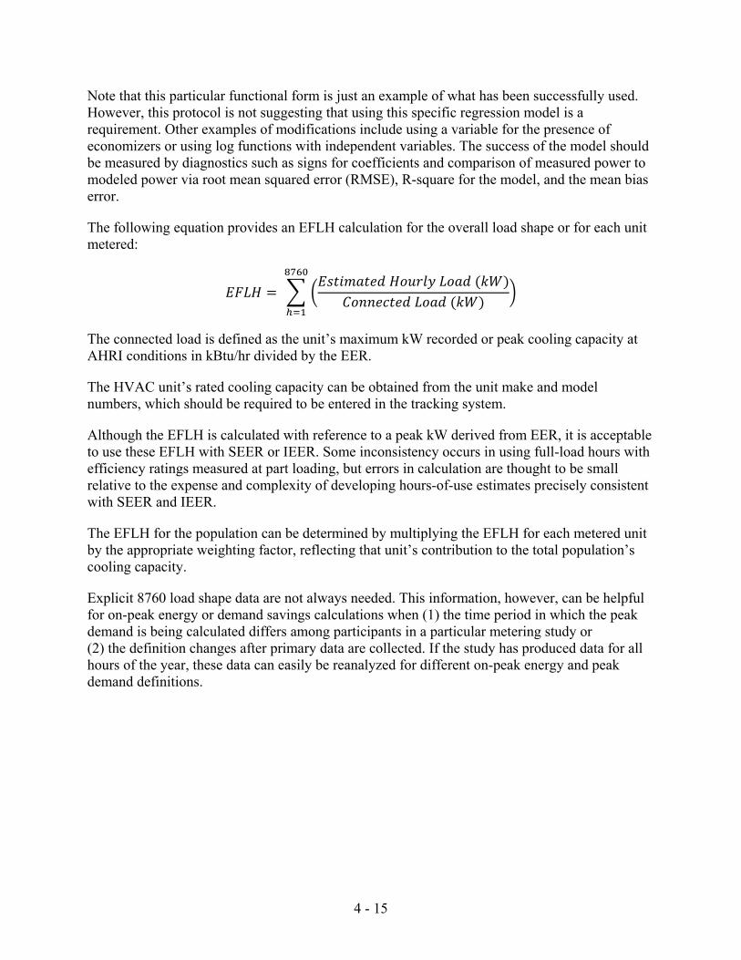
The following equation provides an EFLH calculation for the overall load shape or for each unit metered:

𝐸𝐹𝐿𝐻 = � �𝐸𝑠𝑡𝑖𝑚𝑎𝑡𝑒𝑑 𝐻𝑜𝑢𝑟𝑙𝑦 𝐿𝑜𝑎𝑑 (𝑘𝑊)

𝐶𝑜𝑛𝑛𝑒𝑐𝑡𝑒𝑑 𝐿𝑜𝑎𝑑 (𝑘𝑊) �8760

ℎ=1

The connected load is defined as the unit’s maximum kW recorded or peak cooling capacity at AHRI conditions in kBtu/hr divided by the EER.

The HVAC unit’s rated cooling capacity can be obtained from the unit make and model numbers, which should be required to be entered in the tracking system.

Although the EFLH is calculated with reference to a peak kW derived from EER, it is acceptable to use these EFLH with SEER or IEER. Some inconsistency occurs in using full-load hours with efficiency ratings measured at part loading, but errors in calculation are thought to be small relative to the expense and complexity of developing hours-of-use estimates precisely consistent with SEER and IEER.

The EFLH for the population can be determined by multiplying the EFLH for each metered unit by the appropriate weighting factor, reflecting that unit’s contribution to the total population’s cooling capacity.

Explicit 8760 load shape data are not always needed. This information, however, can be helpful for on-peak energy or demand savings calculations when (1) the time period in which the peak demand is being calculated differs among participants in a particular metering study or (2) the definition changes after primary data are collected. If the study has produced data for all hours of the year, these data can easily be reanalyzed for different on-peak energy and peak demand definitions.

4 - 16

5 Sample Design Evaluators will determine the required targets for confidence and precision levels, subject to specific regulatory or program administrator requirements. In most jurisdictions, the generally accepted confidence levels should be designed to estimate EFLH with a sampling precision of 10% at the 90% confidence interval. If attempting to organize the population into specific subgroups (such as building types or unit sizes), it may be appropriate to target 20% precision with a 90% confidence interval for individual subgroups, and 10% precision for the large total population.

In addition to sampling errors, errors in measurement and modeling can also occur. In general, these errors are lower than the sampling error; thus, sample sizes commonly are designed to meet sampling precision levels alone.

Sample sizes for achieving this precision level should be determined by estimating the coefficient of variation (CV), calculated as the standard deviation divided by the mean. CVs generally range from 0.5 to 1.06, and the more homogeneous the population, the lower the likely CV. After the study is completed, the CV should be recalculated to determine the actual sampling error of the metered sample.

As discussed, units should be sampled based on climate zones and unit sizes, if sufficient variation occurs in these quantities. Alternatively, the most prevalent building types can be sampled if the program administrator’s database tracks building types accurately. One overall EFLH average can be developed if most units lie within a single climate zone and have a narrow range in capacity.

Many customers taking advantage of unitary HVAC rebate programs have multiple air-conditioning units rebated simultaneously. Consequently, the sampling plan must consider whether a sample can be designed for specific units, groups of units by size, or all units at a given site. It is also important to consider the resources needed to schedule and send metering technicians or engineers to a given site. Once those fixed costs have been incurred, metering multiple units at a site becomes an attractive option.

Decisions on how best to approach site (facility) sampling versus unit sampling depend on the degree of detail in the information available for each unit rebated. In many cases, rebate applications and tracking systems only record the total number of units in each size category, rather than the specific information on the location of each unit. For these instances, develop a specific rule that calls for random sampling of a fixed percentage of units at a given site.

Based on these considerations, sampling should be conducted per-customer site or application, with a specified minimum number of units sampled at a given site. A reasonable target is two or more units in each size category at each site with multiple units.

6 At a CV of 0.5, the sample size to achieve a 10% precision with a 90% confidence interval is 67. At CV of 1.0,

the sample size is 270.

4 - 17

6 Program Evaluation Elements To assure the validity of data collected, establish procedures at the beginning of the study to address the following issues:

• Quality of an acceptable regression curve fit (based on R2, missing data, etc.)

• Procedures for filling in limited amounts of missing data

• Meter failure (the minimum amount of data from a site required for analysis)

• High and low data limits (based on meter sensitivity, malfunction, etc.)

• Units to be metered not operational during the site visit (For example, determine whether this should be brought to the owner’s attention or whether the unit be metered as is.)

• Units to be metered malfunction during the mid-metering period and have (or have not) been repaired at the customer’s instigation.

It is recommended to add to the sample an additional 10% of the number of sites or units to account for data attrition.7

At the beginning of each study, determine whether metering efforts should capture short-term measure persistence. That is, decide how the metering study should capture the impacts of non-operational rebated equipment (due to malfunction, cooling no longer needed, equipment never installed, etc.). For non-operational equipment, these could either be treated as equipment with zero operating hours, or a separate assessment could be done of the in-service rate.8

One key issue is how to extrapolate data beyond the measurement period for units that may be left on after the primary cooling season ends. To address this and other unique operating characteristics, conduct site interviews with facility managers or homeowners (for residential units), as customers often know when units have been and are typically turned off for the season. These interview data can be used to override regression analysis indicating usage in the off-season, provided the customer can be certain the unit has not operated.

In analyzing year-round data from a mid-Atlantic utility, KEMA found that once the THI fell below 50oF, most units shut off for the season. That information enabled KEMA to apply this rule to other sites in the NEEP EM&V Forum study, resulting in a more realistic estimate of fall and winter cooling hours than was obtained by applying only regression results.

6.1 Net-to-Gross A separate cross-cutting protocol to determine applicable net-to-gross is planned for Phase 2 of the Uniform Methods Project.

7 In KEMA’s study for the NEEP EM&V Forum, approximately 9% of metered units were removed due to data

validity problems (KEMA 2011). 8 The “Residential Lighting” protocol further discusses in-service rates.

4 - 18

7 References

ADM. (November 2009). “Residential Central AC Regional Evaluation.” Prepared for NSTAR Electric and Gas Corporation, National Grid, Connecticut Light & Power, and United Illuminating.

Air Conditioning Contractors of America (ACCA). (2007). Standard 5 (ANSI/ACCA 5 QI-207) HVAC Quality Installation Specification.

Air-Conditioning, Heating and Refrigeration Institute (AHRI). (2008). ANSI/AHRI 210/240-2008 with Addendum 1, Performance Rating of Unitary Air-Conditioning & Air-Source Heat Pump Equipment.

American Society of Heating Refrigeration and Air-Conditioning Engineers (ASHRAE). (2000). Compilation of Diversity Factors and Schedules for Energy and Cooling Load Calculations, ASHRAE Research Report 1093.

ASHRAE. (2002). Guideline 14-2002 Measurement of Energy and Demand Savings. (Revision 14-2002R in process).

ASHRAE. (2010). Performance Measurement Protocols for Commercial Buildings. Consortium for Energy Efficiency (CEE). (2009). Commercial Unitary AC and HP Specifications, Unitary Air Conditioning Specification. Effective January 16, 2009. www.cee1.org/com/hecac/hecac-tiers.pdf.

ISO-New England, Inc. (June 2010). ISO New England Manual for Measurement and Verification of Demand Reduction Value from Demand Resources Manual (M-MVDR).

Itron, Inc. (December 2005). 2004-05 Database of Energy Efficient Resources (DEER) Update. Prepared for Southern California Edison.

Itron, Inc. and KEMA. (December 31, 2008). 2004/2005 Statewide Express Efficiency and Upstream HVAC Program Impact Evaluation. Prepared for the California Public Utility Commission, Pacific Gas & Electric Company, San Diego Gas & Electric Company, Southern California Edison, and Southern California Gas Company. www.calmac.org/publications/FINAL_ExpressEfficiency0405.pdf.

KEMA. (2009). Pacific Gas & Electric SmartAC™ 2008 Residential Ex Post Load Impact Evaluation and Ex Ante Load Impact Estimates, Final Report. Prepared for Pacific Gas and Electric. March.

KEMA. (February 10, 2010). Evaluation Measurement and Verification of the California Public Utilities Commission HVAC High Impact Measures and Specialized Commercial Contract Group Programs 2006-2008 Program Year. www.calmac.org/publications/Vol_1_HVAC_Spec_Comm_Report_02-10-10.pdf.

4 - 19

KEMA. (August 2, 2011). C&I Unitary HVAC Load Shape Project. Prepared for the Regional Evaluation, Measurement and Verification Forum facilitated by the Northeast Energy Efficiency Partnerships (NEEP).

Massachusetts Program Administrators. (October 2011). Massachusetts Technical Reference Manual for Estimating Savings from Energy Efficiency Measures 2012 Program Year—Plan Version.

Navigant. (June 2010). “The Sun Devil in the Details: Lessons Learned from Residential HVAC Programs in the Desert Southwest.” Presented at Counting on Energy Programs: It’s Why Evaluation Matters. Paris, France: International Energy Program Evaluation Conference.

Regional EM&V Methods and Savings Assumption Guidelines. (May 2010.) Northeast Energy Efficiency Partnerships (NEEP) EM&V Forum.

SAIC. (1998). New England Unitary HVAC Research Final Report. Sponsored by New England Power Service Company, Boston Edison Company, Commonwealth Electric, EUA Service Company, and Northeast Utilities.

TecMarket Works. (October 15, 2010). New York Standard Approach for Estimating Energy Savings from Energy Efficiency Programs- Residential, Multi-Family and Commercial/ Industrial Measures. Prepared for the New York Public Service Commission. http://efile.mpsc.state.mi.us/efile/docs/16671/0026.pdf.

United Illuminating Company and Connecticut Lighting and Power Company. (October 2008). UI and CL&P Program Savings Documentation for 2009 Program Year.

Vermont Energy Investment Corporation. (August 6, 2010). State of Ohio Energy Efficiency Technical Reference Manual Including Predetermined Savings Values and Protocols for Determining Energy and Demand Savings. Prepared for the Public Utilities Commission of Ohio. http://amppartners.org/pdf/TRM_Appendix_E_2011.pdf.

4 - 20

8 Resources

Consortium for Energy Efficiency (CEE). (January 2010). Information for CEE Program Administrators on the New Part Load Efficiency Metric for Unitary Commercial HVAC Equipment. www.cee1.org/com/hecac/Prog_Guidance_IEER.pdf.

Regional EM&V Methods and Savings Assumption Guidelines. (May 2010.) Northeast Energy Efficiency Partnerships (NEEP) EM&V Forum.