74

Chapter 4

RESEARCH METHODOLOGY

4.1 Introduction

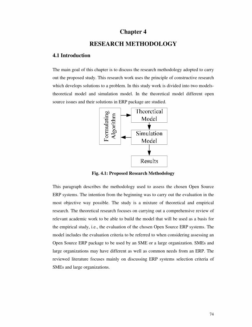
The main goal of this chapter is to discuss the research methodology adopted to carry

out the proposed study. This research work uses the principle of constructive research

which develops solutions to a problem. In this study work is divided into two models-

theoretical model and simulation model. In the theoretical model different open

source issues and their solutions in ERP package are studied.

Fig. 4.1: Proposed Research Methodology

This paragraph describes the methodology used to assess the chosen Open Source

ERP systems. The intention from the beginning was to carry out the evaluation in the

most objective way possible. The study is a mixture of theoretical and empirical

research. The theoretical research focuses on carrying out a comprehensive review of

relevant academic work to be able to build the model that will be used as a basis for

the empirical study, i.e., the evaluation of the chosen Open Source ERP systems. The

model includes the evaluation criteria to be referred to when considering assessing an

Open Source ERP package to be used by an SME or a large organization. SMEs and

large organizations may have different as well as common needs from an ERP. The

reviewed literature focuses mainly on discussing ERP systems selection criteria of

SMEs and large organizations.

75

Fig. 4.2: The Methodology

The literature review aims to put forth a list of “dimensions” which represent one of

the two components of the evaluation model. The other component is the set of

“features” which were identified by looking at the feature offering of the ERP

systems. Once the theoretical study is completed, the model for evaluating the Open

Source ERP systems is built based on the “dimensions” and “features” identified

through the literature study and the study of the ERP systems themselves. The model

serves as the guiding principle when examining the ERP systems and collecting the

empirical data. The evaluation of the systems based on the “dimensions” is performed

in a qualitative way, and was fed by searching the documentation published on the

vendors’ websites and also by evaluating the systems themselves after downloading

them and installing them.

4.2 Research Design

Software reliability is also important factor affecting system reliability where a

system as an entity provides defined behavior at interfaces. A System is a hierarchy of

subsystems, each subsystem being a system. The reliability of a system is its ability to

provide failure-free operation. Failure is the system behavior which is incorrect or not

as expected. It is a random phenomenon.

The following steps are carried out:

1. Presumption of the precise field from where the error may present or remain.

2. Implementing software testing.

3. Catching the error by using PSS (Procedure, System, and Schemes) of testing.

4. Select the error type as per the development lifecycle.

76

5. Choosing suitable software reliability model for that specific stage of error.

6. Applying the reliability models for mitigating errors.

Generally, the proposed software reliability is classified into three phases:

1. Probing predicament (like testing and analyzing errors, malfunction, error

and defects, etc.): This is the first phase of software reliability scheme. In this

step, we are implementing testing and comparing the performance of software

with its preceding standards. By using different types of testing such as black

box and white box testing, we catch the problem occurring. If we catch the

problem we go to next phase of PSS for predicting, removing and solving the

problem.

2. Applying PSS (Procedure, System, and Schemes for solving, predicting or

eliminating the issue): After successful completion of the probing predicament

stage, we apply the PSS which is a collection of techniques, approaches and

methods. The availability of such techniques ensures better mitigation

capability in various issues in software. We also apply few important

approaches for solving these problems.

a. Approaches:- For selecting the SR model and to predict the software

from failure and faults, these are two important approaches:

i. The first approach should be selection of model for classifying

Software Reliability on the basis of adopted SDLC. The

process should ensure the status of upcoming problem i.e., in

which phase of SDLC the problem is occurred. Then we apply

related SR model for that phase to predict the software [93].

ii. The second approach should be distinguishing the association

between SR model and parameters estimations procedure by

using predicting performance.

b. Techniques: - Generally in searching the problem, two testing

techniques are applied. These techniques are

i. Black box testing

ii. White box testing

3. Methods: - By the help of methods we are finding approaches and techniques.

It means they are inter-related to each other. The G.J. Knafl [94] gave the

systematic approach to software reliability model.

77

4. Confirming and authenticating these PSS. (So that, we say that by applying

PSS we ensure and maximize the assurance about reliability of software.)

4.3 Proposed Algorithm

Step 1:-We will guess a few areas where fault may occur. By using simple testing we

increase our guessing probability that the fault still remains in that particular area.

Finally we guess right areas, where fault may be present or remains. We use few

searching methods for searching these problems and catch the problem.

Step 2:- When problem is searched or fetched, we apply PSS (Procedure, System, and

Schemes) to solve these problems. Select the categories of the problem by using the

basic concept of failure. It may be due to clerical error, testing error, coding error

and design error.

2 (a) If it is a clerical type of error, use a systematic approach to remove the

problem.

2 (b) If it is a testing type of error, then use two testing technique to remove these

problem.

b1. Unit testing

b2. Integration testing

b3. System testing

2 (c) If it is coding or design type of error, then use few methods (or appropriate

methodology) to solve these problems.

Then

Step 2(b) is performed.

Step 3:- Apply step 2, until the problem is solved, predicted or removed.

Step 4:- Apply verification and validation of these PSS by using some engineering

statistical data. Through these steps ensure and increase the confidence about

software reliability.

4.4 Proposed Schema of Software Reliability

In the proposed model of software reliability, we will collect all the errors which we

have received while performing black box testing and will pass the test parameters to

78

the proposed mathematical model which will use fairly accurate maximum likelihood

function using evolutionary method as well as Monte Carlo technique. For this

purpose, all the error information is plotted, and exponential power factors are

evaluated. A Java testing application is designed for collecting almost all sorts of

errors extracted from OFBiz software application. A real software reliability data set

is considered for illustration of the proposed methodology under informative set of

priors. In this real data set, Time-between failures is converted to time to failures and

scaled. In this research work, we have presented the Exponential Power model as

software reliability model which was motivated by the fact that the existing models

were inadequate to describe the failure process underlying some of the data sets. We

have developed the tools for empirical modeling, e.g., model analysis, model

validation and estimation.

There are two objectives for an error-reporting process. The first is to report the right

information needed for measuring the impact of the errors, and the second is to report

it as efficiently as possible so that the resulting measurement may have impact on the

development process and product. The error or problem-reporting process usually

includes a problem report sheet, and an information flow process between each of the

individuals and organizations responsible for modifying the software. The

responsibility for collecting the data may be divided by various organizations, such as

testing, quality assurance, reliability engineering, software development, system

engineering, etc. An organization flow for data collection is suggested in Figure 4.3.

The problem report should have three parts:

• The error detection section,

• The error correction section, and

• The error correction verification section.

79

Fig. 4.3: Flow chart of a problem reporting process

Error detection information is generally filled out by the testing personnel. These

personnel may be the person who developed the software, another developer, a

completely independent testing person from outside of the organization, an

independent tester from within the organization, a customer, or any person using the

software who detects an error or anomaly in the software. Once the problem is

recorded, the criticality, priority and problem number are assigned by either a quality

assurance person or a lead software engineer. The problem is usually reviewed by a

review board or by the lead software engineer, and it is determined whether or not the

problem is truly an error that must be corrected or whether the problem is rejected for

reasons to be discussed shortly.

80

If the report does indicate a problem that must be fixed, it will be prioritized by its

criticality and the estimated time required to fix it. The report is numbered

sequentially and uniquely so that it can later be traced. The number may also be

assigned so that it distinguishes where the problem was found functionally and who

found it. For example, the first letter in the report number may indicate the group that

found the problem, and the second letter may indicate the function of the software

where the problem seems to be located.

4.5 Proposed Model

In the analysis of lifetime or the survival data the Exponential model plays a vital role

and it happens only due to their convenient statistical theory and even their important

'lack of memory' property. In spite of these the constant hazard rates are also the

dominant reason. On the other hand this is also a fact that in such kind of

circumstances in which the one parameter family of the exponential distribution

model is not enough broad, then numerous wider families like gamma, Weibull

lognormal models are generally implemented. In order to obtain more flexible new

families of the model, the addition of the parameters is done in the well established

family of models, which is a time honored device. This robust power model

(exponential Power model) was introduced by [78] presenting it as a lifetime model.

The same model has been researched, enhanced and discussed by many researches

[4], [9] and [12].

In definition the exponential model can be defined as a model in which the shape

parameter λ>0 and scale parameter α>0. This criterion is considered as the referencing

only in the case of a survival function of the model, that is given as,

),0(,0),(},1exp{)( )( ∞∈>−= xexRx λα

αλ

(4.1)

A. Model Analysis

In order to achieve the parameters like α > 0 and, λ > 0 the two-parameter Exponential

Power model has a distribution function that is represented as below;

0,0),(};1exp{1),;( )( ≥>−−= xexFx λαλα

αλ

(4.2)

Now, the probability density function (PDF) that is allied with equation (4.3) can be

presented as below:

81

0,0),(};1exp{),;( )()(1 ≥>−= −xeexxf

xx λααλλααα λλαα

(4.3)

Generally the Exponential power model with the its dominating parameters α and λ

can be expressed as a function EP (α, λ). In this stating function the parameter α is

indicating the “shape parameter” as stated by [79] and [14]. Meanwhile, the R

functions dexp.power() and pexp.power() is presented n in SoftreliaR package that

can be used for the computation of PDF and CDF, respectively. Here in the extension

some of the typical Exponential Power density functions for different values of shape

parameters α and for λ = 1 is being presented in Figure 4.4. It is clear from the Figure

4.4 that the density function of the Exponential Power model can take different

shapes.

Fig. 4.4: Referencing plot for the probability density function of the Exponential

Power model with the parameters values λ =1 and different values of α

1) Mode

Solving the following non-linear equation, the Mode for the EP model can be

obtained:

0}1{)()1( )( =−+−αλαλαα x

ex (4.4)

2) The Quantile function

Considering a continuous distribution F(x), the p percentile that is referred as a

fractile or the quantile, xp, for a given p, 0 < p <1 can be represented as

P(X<xp) =F (xp) =p (4.5)

82

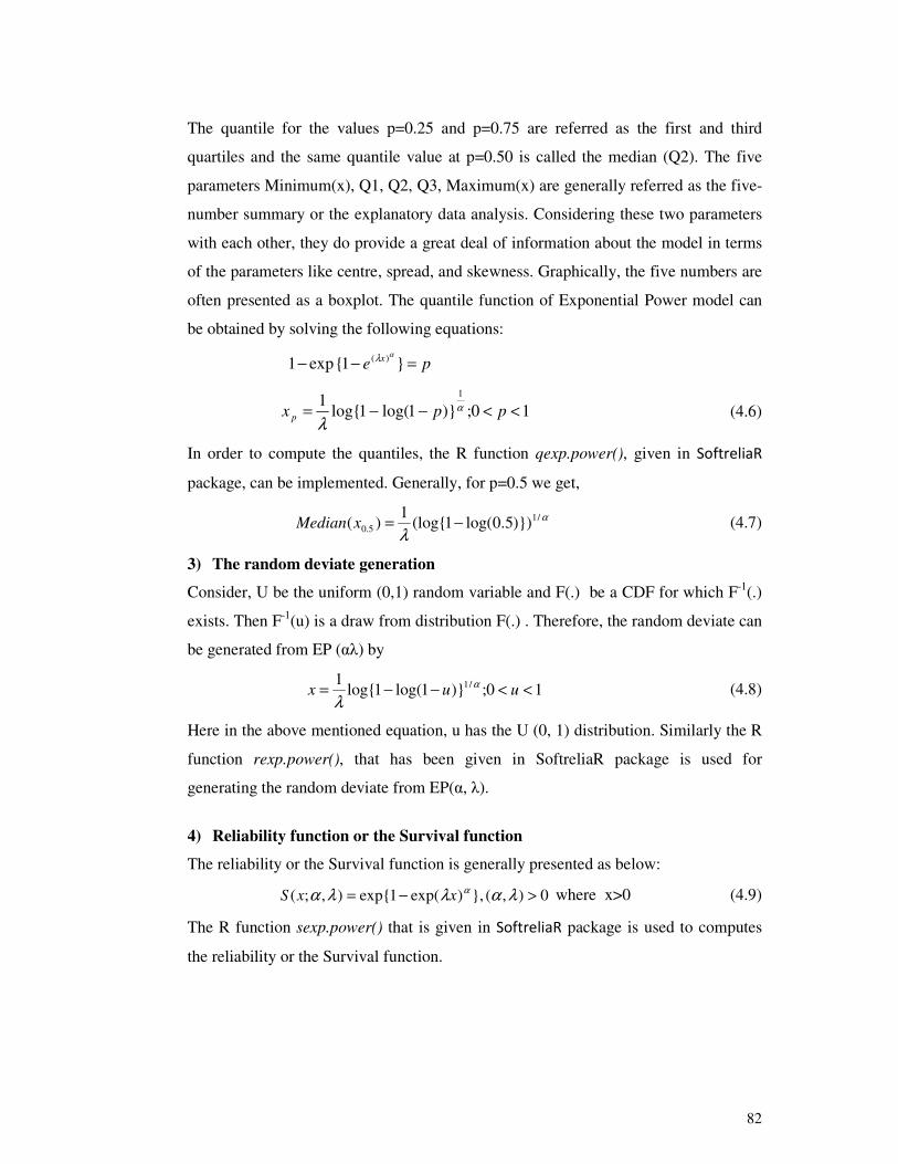
The quantile for the values p=0.25 and p=0.75 are referred as the first and third

quartiles and the same quantile value at p=0.50 is called the median (Q2). The five

parameters Minimum(x), Q1, Q2, Q3, Maximum(x) are generally referred as the five-

number summary or the explanatory data analysis. Considering these two parameters

with each other, they do provide a great deal of information about the model in terms

of the parameters like centre, spread, and skewness. Graphically, the five numbers are

often presented as a boxplot. The quantile function of Exponential Power model can

be obtained by solving the following equations:

pe x =−− }1{ exp1 )( αλ

10;)}1log(1log{1

1

<<−−= ppx pα

λ (4.6)

In order to compute the quantiles, the R function qexp.power(), given in SoftreliaR

package, can be implemented. Generally, for p=0.5 we get,

α

λ/1

5.0 )})5.0log(1(log{1

)( −=xMedian

(4.7)

3) The random deviate generation

Consider, U be the uniform (0,1) random variable and F(.) be a CDF for which F-1(.)

exists. Then F-1(u) is a draw from distribution F(.) . Therefore, the random deviate can

be generated from EP (αλ) by

10;)}1log(1log{1 /1 <<−−= uux

α

λ (4.8)

Here in the above mentioned equation, u has the U (0, 1) distribution. Similarly the R

function rexp.power(), that has been given in SoftreliaR package is used for

generating the random deviate from EP(α, λ).

4) Reliability function or the Survival function

The reliability or the Survival function is generally presented as below:

0),(},)exp(1exp{),;( >−= λαλλα αxxS where x>0 (4.9)

The R function sexp.power() that is given in SoftreliaR package is used to computes

the reliability or the Survival function.

83

5) The Hazard Function

The Hazards function also plays a vital role in stating the reliability of the Exponential

power function. The hazard function of Exponential Power model is given by

0),(,)exp(),;( 1 >= − λαλαλλα ααα xxxh And x>0 (4.10)

The shape of the hazard function h(x) depends on the value of the shape parameter α.

Therefore when α ≥ 1, the failure rate function is generally increasing. Similarly,

when α < 1, the failure rate function is of bathtub shape. These illustrations indicate

that the shape parameter α plays an important role for the model.

Differentiating the hazards function as mentioned above w.r.to x, we find

})()1{(1

)(' αλαα xx

xh +−=

(4.11)

Now, putting h’(x) = 0 and Simplifying it, we get the change point which is presented

as

α

α

α

λ/1

0 )1

(1 −

=x (4.12)

It easily follows that the sign of h’(x) is calculated by (α-1) +α(λx)α which is negative

for all x≤x0 and positive for all x>x0.

Fig. 4.5: Plots of the hazard function of the Exponential Power model for λ=1

and different values of α.

84

Some of the typical Exponential Power Model hazard functions for different values of

α and for λ= 1 have been illustrated in Figure 4.5. The Figure 4.5 also illustrates that

the hazard function of the Exponential Power model can have many shapes depending

on the shape parameters.

6) The cumulative hazard function

The cumulative hazard function H(x) defined as

H(x) =-{1-log (F(x))} (4.13)

The CHF can be achieved with the help of pexp.power() function and that is

mentioned in SoftreliaR package by choosing arguments lower.tail=FALSE and

log.p=TRUE. i.e. - pexp.power(x, alpha, lambda, lower.tail = FALSE, log.p =

TRUE)

7) Failure rate average (FRA) and Conditional Reliability Function (CRF)

In spite of the above mentioned parameter function there are two other relevant

functions that are useful in reliability analysis. These functions are failure rate average

(FRA) and conditional survival function (CRF) The failure rate average of X is given

by

FRA(x) = H(x) / x, x > 0 (4.14)

where H(x) refers to the cumulative hazard function.

The survival function (S.F) and the conditional survival of X are defined by

R(x)=1-F(x)

and R(x|t)=R(x+t)/R(x) t>0, x>0, R(.)>0,

(4.15)

Respectively, where F(·) presents the CDF of X, similarly to hazards function h(x)

and the failure rate average FRA(x), the distribution of X belongs to the new better

than used (NBU), exponential, or new worse than used (NWU) classes, when R (x | t)

< R(x), R(t | x) = R(x), or R(x | t) > R(x), respectively.

The R functions hra.exp.power() and crf.exp.power() that is mentioned in SoftreliaR

package can be used for the failure rate average (FRA) and Conditional Reliability

Function(CRF), respectively.

85

4.6 Bayesian Estimation in FindBug

The dominant software tool that is applied for Bayesian inference is the FindBug. The

main characteristic of this software tool is that it is a fully extensible modular

framework for constructing and analyzing Bayesian full probability models.

Meanwhile this OSS (Open Source Software) requires the incorporation of a module

to evaluate the parameters of the Exponential power model. The dexp.power_T

(alpha, lambda) is written in component Pascal, that facilitates to perform full

Bayesian analysis of Exponential Power model into FindBug using the method

described in [15] and [10].

1. Implementation of Module - dexp.power_T(alpha, lambda)

In order to obtain the Bayes estimates of the Exponential Power model using MCMC

method dexp.power_T (alpha, lambda) module has been implemented. The dominant

function of this developed module is to generate MCMC sample from posterior

distribution under informative set of priors, i.e. Gamma priors.

A. Data Analysis

In this research work we have been using the software reliability data set SYS2.DAT

– 86 time-between-failures [10] is considered for illustration of the proposed

methodology. In this real data set, Time-between failures is converted to time to

failures and then it is scaled.

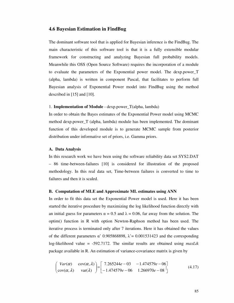
B. Computation of MLE and Approximate ML estimates using ANN

In order to fit this data set the Exponential Power model is used. Here it has been

started the iterative procedure by maximizing the log likelihood function directly with

an initial guess for parameters α = 0.5 and λ = 0.06, far away from the solution. The

optim() function in R with option Newton-Raphson method has been used. The

iterative process is terminated only after 7 iterations. Here it has obtained the values

of the different parameters α’ 0.905868898, λ’= 0.001531423 and the corresponding

log-likelihood value = -592.7172. The similar results are obtained using maxLik

package available in R. An estimation of variance-covariance matrix is given by

−−−

−−−=

08266970.106474579.1

06474579.103265244.7

)var(),cov(

),cov()(

ee

eeVar

λλα

λαα (4.17)

86

Thus using the above mentioned eq. (4.17), the approximate 95% confidence intervals

for the parameters of EP model based on MLEs can be estimated. Table 4.1 illustrates

the MLEs with their standard errors and approximate 95% confidence intervals for α

and λ.

Table 4.1: Maximum Likelihood Estimate, Standard Error and 95% Confidence

Interval

Parameter MLE Std. Error 95% Confidence Interval

Alpha 0.905868 0.085236 (0.7388055, 1.0729322)

Lambda 0.001531 0.000112 (0.0013108, 0.0017520)

An approximate ML estimates that is based on Artificial Neural Networks (ANN) are

obtained by using the neuralnet package that is available in R. Here one hidden- layer

feed forward neural networks with sigmoid activation function has been selected. The

results are quite close to exact ML estimates.

4.7 Model Validation

In order to study the better features of the fit of the Exponential Power model, here

the Kolmogorov-Smirnov statistic between the empirical distribution function and the

fitted distribution function has been estimated and it is computed when the parameters

are obtained by method of maximum likelihood. For this R function ks.exp.power( ),

given in SoftreliaR package can be implemented. The result of K-S test is D = 0.0514

with the corresponding p-value = 0.9683, Therefore, the high p-value strictly states

that the Exponential Power model can be used to analyze this data set, and plot the

empirical distribution function and the fitted distribution function can be obtained that

has been presented in Figure 4.6. From above result and Figure 4.6, it is clear that the

estimated Exponential Power model provides excellent fit to the given data.

87

0 200 400 600 800

0.0

0.2

0.4

0.6

1000

0.8

1.0

x

f(x)

Fig. 4.6: Empirical distribution and fitted distribution function.

The other graphical method that is widely used for verifying whether a fitted model is

in conformity with the data is Quantile-Quantile (Q-Q) plots.

Figure 4.7 Quantile-Quantile (Q-Q) plot using MLEs as estimate.

As depicted in the above mentioned figure the Q-Q plots illustrate the estimated

versus the observed quantiles. If the model fits the data in a better way, the pattern of

points on the Q-Q plot exhibits a 45-degree straight line.

Note that all the points of a Q-Q plot are lying inside the square

[F-1(p1:n),F-1(pn:n)] x [x1:n,xn:n]

88

The corresponding R function qq.exp.power() has been provided in the SoftreliaR

package. The straight line pattern in Figure 4.7, states that the Exponential Power

model fits the data very well.

Here in order to generate two Markov Chains at the length of 40,000 with different

starting points of the parameters, the convergence can be monitored by using trace

and ergodic mean plots. Here it can be found that the Markov Chain converge

together after approximately 2000 observations. Therefore, usage of 5000 samples is

more than enough to erase the effect of starting point (initial values). At last the

samples of size 7000 are formed from the posterior by picking up equally spaced

every fifth outcome, i.e. thin=5, starting from 5001. This is done only for minimizing

the auto correlation among the generated deviates. Therefore, the values that can be

obtained are the posterior sample {α1i, λ1i}, i = 1,…,7000 from chain 1 and α2i , λ2i}, i

= 1,…,7000 from chain 2. The chain 1 is considered for convergence diagnostics

plots. The visual summary is based on posterior sample obtained from chain 2

whereas the numerical summary is presented for both the chains.

A. Convergence diagnostics

The Sequential realization of the parameters α and λ can be experiential in figure 4.8.

The Markov chain is most liable to be sampling from the stationary distribution and is

mixing well.

1) History(Trace) plot

Fig. 4.8: Sequential realization of the parameters α and λ

89

There is abundant substantiation of convergence of chain as the plots show no long

upward or downward trends; rather it looks like a horizontal band, then it can be

proved that it is getting converged.

2) Running Mean (Ergodic mean) Plot

The convergence pattern which is solely depends on the Ergodic average has been

presented in figure 4.9. It is obtained after generating a time series (Iteration number)

plot of the running mean for each parameter in the chain. The running mean is

computed as the mean of all sampled values up to and including that at a given

iteration.

Fig. 4.9: The Ergodic mean plots for α and λ

3) Autocorrelation

Here the plotted graph illustrates that the correlation is almost negligible and thus it

can be concluded that the samples are independent.

Fig. 4.10: The autocorrelation plots for α and λ.

90

4) Brooks-Gelman-Rubin Plot

This implements the parallel chains with dispersed initial values so as to test whether

they all converge to the same target distribution or not. Here the failure could indicate

the presence of a multi-mode posterior distribution that is different chains converge to

different local modes or the need to run a longer chain which is the burn-in is yet to be

completed.

Fig. 4.11: The BGR plots α and λ.

As depicted in the above mentioned figure 4.11, it is clear that convergence is

achieved. Thus the posterior summary statistics can be obtained.

B. Visual summary

1) Box plots

In this type of plot presentation the boxes represent the inter-quartile ranges and the

solid black line at the centre of each box is the mean; the arms of each box extend to

cover the central 95 per cent of the distribution - their ends correspond, therefore, to

the 2.5% and 97.5% quantiles.

Fig. 4.12: The boxplots for alpha and lambda.

91

2) Kernel density estimates

A histogram plays a vital role in providing the insights on symmetric, behavior in the

tails, presence of multi-modal behavior, and data outliers. Histograms can be

compared to the fundamental shapes that are associated with standard analytic

distributions.

Fig. 4.13: Kernel density estimate and histogram of α based on MCMC samples,

vertical lines present the corresponding ML and Bayes estimates.

Here the depicted figures (Figure 4.13 and 4.14) provide the kernel density estimate

of α and λ respectively. Here it can be seen that α and λ both are symmetric.

Fig. 4.14: Histogram and kernel density estimate of λ based on MCMC samples

92

C. Comparison with MLE

In order to compare the model with MLE, here two graphs have been plotted. In

Figure 4.15, the density functions f(x; α’, λ’) are plotted using MLEs and Bayesian

estimate. Then they are, computed via MCMC samples under gamma priors,

Fig. 4.15: The density functions f(x; α’, λ’) using MLEs and Bayesian estimates,

computed via MCMC samples under gamma priors.

The Figure 4.16 represents the dashed function that is also known as the estimated

reliability function has been plotted, using the Bayes estimate under gamma priors

and the empirical reliability function (solid line).

Fig. 4.16: The estimated reliability function (dashed line) and the empirical

reliability function (solid line).

From the above mentioned figures it is clear that the MLEs and the Bayes estimates

with respect to the gamma priors are quite close and fit the data very well.

93

4.8 Summary

In this research work, a robust model called Exponential Power model as software

reliability model has been presented which was motivated by the fact that the existing

models were inadequate to describe the failure process underlying some of the data

sets. Here a tool has been developed for empirical modeling that is model analysis,

model validation and estimation. The accurate and precise as well as approximate ML

estimates has been obtained by using ANN of the parameters alpha (α) and lambda

(λ). Here it has been tried to estimate the parameters in Bayesian setup using MCMC

simulation method under gamma priors. The proposed and hence the developed

methodology has been implemented on a real data set. Here both the, numerical

summary and visual summary under different priors have been presented. They

consist the Box plots, Kernel density estimates based on MCMC samples. Similarly

the Bayes estimates have been compared with MLE. Here it has been demonstrated

that the Exponential Power model is suitable for modeling the software reliability data

and thus the tools developed for analysis can also be used for any other type of data

sets.