Embed Size (px)
Citation preview

Part II
FINANCIAL APPLICATIONS
4. Stochastic calculus
5. Option pricing models
6. Interest rate models
Chapter 4
Stochastic calculus
- Brownian motion
- Stochastic integral
- Stochastic differential
- Change of probability measure

Brownian motion
- Definition
o Argument
o Definition
- Properties
o Elementary properties
o Quadratic variation of a SBM
o Regularity properties
- Simulation of a SBM
- Associated BM
o Arithmetic BM
o Brownian bridge
- BM and martingales
o Examples of martingales
o Reciprocal
o Exponential BM
o Using BM as a “noise”
- Hitting time for a SBM
o Definition and property
o Reflection principle
o Distribution of hitting time and maximum
Definition
Argument
Let us consider a (discrete time) symmetrical
random walk (��)
�� = � ��
�� ��~ �−Δ� Δ�12 12 �
with
- � = � ∙ ∆�
- independent moves
- �� = 0
We know that
�(��) = 0
���(��) = (Δ�)�Δ� ∙ �
−Δ� Δ�

We want to define
- a continuous time stochastic process
- with positive constant instantaneous variance
o if ���(��) → ∞, too “explosive” : the
fluctuations will grow to infinity
o if ���(��) → 0, no more random
So, we have to
- let ∆� tend to 0
- in such a manner that ("#)$
"� ∙ � → % ∙ �
We can choose % = 1 : if we want another
constant &, we will consider (&��)
Thanks to the CLT, we have
�� = � ��
�� → '(0; �)
Furthermore, a random walk has independent and
stationary increments …
Definition
A continuous time stochastic process ()�) is a
standard brownian motion (SBM) if
- )� = 0
- ()�) has independent increments
- ()�) has stationary increments
- )� ~ '(0; �)
The notation “)” is for Wiener
Strictly speaking, a Wiener process on a
probability space (Ω, ℱ, Pr, /) is a SBM adapted
to the filtration /
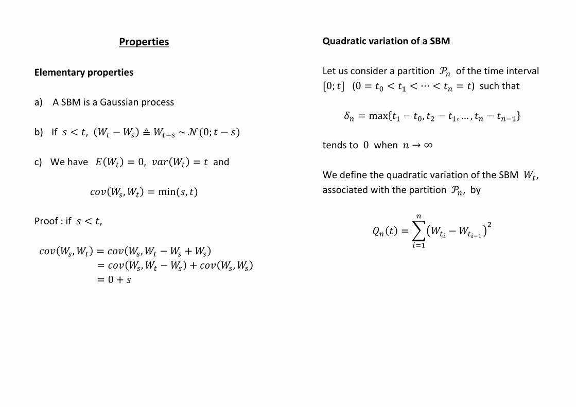
Properties
Elementary properties
a) A SBM is a Gaussian process
b) If 0 < �, ()� − )2) ≜ )�42 ~ '(0; � − 0)
c) We have �()�) = 0, ���()�) = � and
56�()2, )�) = min (0, �)
Proof : if 0 < �,
56�()2 , )�) = 56�()2, )� − )2 + )2)
= 56�()2, )� − )2) + 56�()2, )2)
= 0 + 0
Quadratic variation of a SBM
Let us consider a partition ; of the time interval [0; �] (0 = �� < �� < ⋯ < � = �) such that
? = maxB�� − ��, �� − ��, … , � − �4�D
tends to 0 when � → ∞
We define the quadratic variation of the SBM )�,
associated with the partition ;, by
E(�) = �F)�G − )�GHIJ�
K�

Property : when � → ∞, we have E(�) L.N.OPQ �
Lemma : if �~'(0; &�), then ���(��) = 2&R
Since SR = 3&R, we have
���(��) = �(�R) − ��(��) = 3&R − (&�)�
Proof
• �FE(�)J = ∑ � VF)�G − )�GHIJ�WK�
= ∑ (�K − �K4�)K�
= �
• ���FE(�)J = ∑ ��� VF)�G − )�GHIJ�WK�
= 2 ∑ (�K − �K4�)�K�
≤ 2? ∑ (�K − �K4�)K�
= 2�?
→ 0
so that �((E(�) − �)�) → 0
Regularity properties
a) The paths of a SBM are continuous
We have to prove that lim"�→� )�Z"� = )�
We give a proof for limit in probability. Let us
choose an arbitrary [ > 0. We will prove that
lim"�→� Pr[|)�Z"� − )�| > [] = 0
Since (Chebyshev’s inequality)
Pr^|)�Z"� − )� − 0| > ℎ√Δ�a ≤ 1ℎ�
we have
Pr[|)�Z"� − )�| > [] ≤ Δ�[� → 0

b) The paths of a SBM are nowhere derivable
)�Z"� − )� ~ '(0; ∆�) ≜ √∆� ∙ �
with � ~ '(0; 1)
)�Z"� − )�∆� ≜ �√∆�
that tends to ±∞, depending on the sign of �
Interpretation of this property : a SBM is
unpredictable over short time intervals
c) A SBM has unbounded variations. More
precisely (with the same notations as for
quadratic variation),
c� = sup;g�h)�G − )�GHIh
K�= +∞ �. 0.
If c� were finite (= %, say), then, for any
partition ;,
E(�) = ∑ F)�G − )�GHIJ�K�
≤ ∑ h)�G − )�GHIhK� ∙ maxi�,…, j)�k − )�kHIj ≤ % ∙ maxi�,…, j)�k − )�kHIj
and the 2nd
factor tends to 0 by continuity of the
paths of the SBM. This is incompatible with the
property of quadratic variation : E(�) → �

d) Self-similarity of a SBM
(= scaling effect = “fractals” property)
By definition, a stochastic process is l-self-similar
if, for any � ≥ 1, ��, … , � ∈ o and p > 0,
F�q�I , … , �q�g J ≜ Fpr��I , … , pr��g J
l is the Hurst index of the stochastic process
Property : a SBM is ��-self-similar :
F)q�I , … , )q�g J ≜ F√p)�I , … , √p)�I J
Proof (for � = 1) :
)q� ~ '(0; p�) ≡ √p ∙ '(0; �) ~ √p ∙ )�
Interpretation : the pattern of any path of a SBM
has a similar shape, independently of the length of
the time interval
Simulation of a SBM
It is easy to obtain pseudo-random values for the
law of � from t(0; 1� pseudo-random values :
uv4��w� ≜ �
Pr<uv4��w� X �= � Pr<w X uv���= � uv���

For simulating a path of a SBM, we discretize the
time variable : let the time interval <0; �= be
partitioned in � sub-intervals of length Δ� : � � � ∙ Δ�
We know that
)"� , �)�"� −)"��, … , �)"� −)�4��"��
are i.i.d. r.v. ~'�0; ��
Algorithm :
- Generate � pseudo-random values x�, … , x
values of a t�0; 1� r.v.
- Take the reciprocal of these values to obtain
pseudo-random normal values
)i"� −)�i4��"� � uy4��xi ; 0, Δ�� - Cumulate these values
)�"� � ∑ F)i"� −)�i4��"�J�i�
- Using continuity of the path, connect the
points by line segments
-0,5
-0,4
-0,3
-0,2
-0,1
0
0,1
0 0,02 0,04 0,06 0,08 0,1 0,12 0,14 0,16 0,18 0,2
Simulated standard brownian motion

Associated BM
Arithmetic BM
An ABM with drift z (∈ ℝ) and volatility & (> 0), associated to the SBM ()�), is a
stochastic process (��) defined by
�� = z� + &)�
Properties
- An ABM is a Gaussian process
- Moments : Sv(�) = z� &v�(�) = &�� 5v(0, �) = &� min(0, �)
This process can be generalized for beginning at a
value �� instead of 0 :
�� = �� + z� + &)�
Brownian bridge
A Brownian bridge over the time interval [0; 1],
associated to the SBM ()�), is a stochastic
process (��) defined by
�� = )� − �)�
Properties
- A Brownian bridge is a Gaussian process
- �� = �� = 0
- Moments : Sv(�) = 0 &v�(�) = �(1 − �) 5v(0, �) = min(0, �) − 0�
For the covariance function,
5v(0, �) = 56�()2 − 0)�, )� − �)�)
= min(0, �) − 0 min(1, �)
−� min(0, 1) + 0� min(1, 1)
= min(0, �) − 0�

Brownian motion and martingales
Let us consider a probability space (Ω, ℱ, Pr, /)
where / is the natural filtration of a SBM ()�)
(In this section, we will suppose 0 ≤ 0 < �)
Examples of martingales
a) ()�) is a martingale
�()�|ℱ2) = �()� − )2 + )2|ℱ2)
= �()� − )2|ℱ2) + �()2|ℱ2)
= �()� − )2) + �()2|ℱ2)
= 0 + )2
b) ()�� − �) is a martingale
�()�� − �|ℱ2) = �()�� − )2� + )2�|ℱ2) − �
= �()�� − )2�|ℱ2)
+�()2�|ℱ2) − �
= �()�� − )2�|ℱ2) + )2� − �
But, )�� − )2� = ()� − )2)� + 2)2()� − )2)
so that
�()�� − )2�|ℱ2)
= �(()� − )2)�|ℱ2) + 2�()2()� − )2)|ℱ2)
= (� − 0) + 2)2 �()� − )2|ℱ2)
= (� − 0) + 2)2 �()2 − )2)
= � − 0
and we have
�()�� − �|ℱ2) = (� − 0) + )2� − �
= )2� − 0

c) Counter-example : ()�|) is not a martingale
We know that
�(()� − )2)||ℱ2) = �(()� − )2)|) = 0
0 = �()�| − 3)��)2 + 3)�)2� − )2||ℱ2)
= �()�||ℱ2) − 3)2�()��|ℱ2)
+3)2��()�|ℱ2) − )2|
= �()�||ℱ2) − 3)2�(()�� − �) + �|ℱ2) +3)2�)2 − )2|
= �()�||ℱ2) − 3)2[()2� − 0) + �] + 2)2|
= �()�||ℱ2) − )2| + 3)2(0 − �)
so that �()�||ℱ2) = )2| − 3)2(0 − �) ≠ )2|
Reciprocal (without proof)
If a stochastic process (��) is such that (��) and (��� − �) are martingales, then (��) is a SBM
Exponential Brownian motion
An EBM is a stochastic process (��) defined by
�� = ~���4�$��
with & > 0
Property : an EBM is a martingale
�(~���|ℱ2) = �F~�(��4��) ∙ ~���|ℱ2J
= ~��� ∙ �F~�(��4��)|ℱ2J
= ~��� ∙ �F~�(��4��)J
= ~��� ∙ ~�$(�H�)$
so that
�(��|ℱ2) = � �~���4�$�$ �ℱ2�
= ~��� ∙ ~�$(�H�)$ ∙ ~4�$�$
= ~��� ∙ ~4�$�$
= �2

Particular case : if 0 = 0,
� �~���4�$�� � = �� = 1
Using BM as a “noise”
Objective : express a stochastic process (��) as
the “superposition” of
- a deterministic function ��
- a non predictable “noise” (= martingale)
We can use
a) a SBM as an additive random noise : �� = �� + &)�
b) An EBM as a multiplicative random noise :
�� = �� ∙ ~���4�$��
In both case, �(��) = ��
Hitting time for a SBM
Definition and property
For any fixed � > 0, we define the hitting time o�
as the first time the SBM )� hits the value � :
minB� ∈ o ∶ )� = �D
(and +∞ if )� ≠ � ∀� ∈ o)
Property : the hitting time is a stopping time
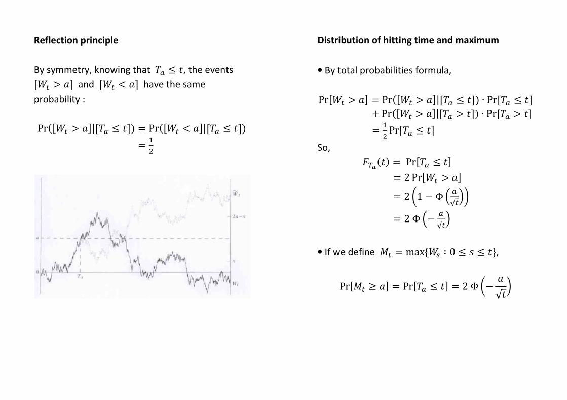
Reflection principle
By symmetry, knowing that o� ≤ �, the events [)� > �] and [)� < �] have the same
probability :
Pr�<)� \ �=|<o� X �=� � Pr�<)� 1 �=|<o� X �=�
� �
�
Distribution of hitting time and maximum
• By total probabilities formula,
Pr[)� > �] = Pr([)� > �]|[o� ≤ �]) ∙ Pr[o� ≤ �]
+ Pr([)� > �]|[o� > �]) ∙ Pr[o� > �]
= �� Pr[o� ≤ �]
So,
u��(�) = Pr[o� ≤ �]
= 2 Pr[)� > �]
= 2 �1 − Φ V �√�W�
= 2 Φ V− �√�W
• If we define �� = maxB)2 ∶ 0 ≤ 0 ≤ �D,
Pr[�� ≥ �] = Pr[o� ≤ �] = 2 Φ �− �√��

Stochastic integral
- Definition
o Motivation
o Classical Riemann integral
o Stieltjes-Riemann integral
o Generalization ?
o Choice of a definition
o Definition
- Properties
o Conditions of existence
o Properties
Definition
Motivation
- The definition of the integral of a function �(�) is concerned with small variations of the
variable �
- The definition of the differential of a function � (��(�) = �′(�) ∙ ��) is also concerned
with small variations of the variable �
Here, we will look at the time variations “through
a SBM”, which has
- unbounded variations
- non differentiable paths
The convergence being no more defined in the
classical way, we have to give new definitions

Classical Riemann integral
Let ; be a partition of [�; �=
� � �� 1 �� 1 ⋯ 1 �4� 1 � � �
with
�K − �K4� � ΔK
? � max�Δ�,Δ�, … ,Δ�
and let choose xK ∈ =�K4�; �K<
The Riemann integral is defined by
� ��x��x = lim→Z∞�g→� � �(xK) ∙ ΔKK�
��
It can be prove that if � is sufficiently “regular”
(continuous by parts e.g.), this integral
- exists
- is independent of ;
- is independent of the choice of xK in =�K4�; �K[

Stieltjes-Riemann integral
This is the same notion as ordinary Riemann
integral, but the measure along horizontal axis is
no more the length of segments, but the length
through another function �
� ��x� ��(x)��
= lim→Z∞�g→� � �(xK) ∙ F�(�K) − �(�K4�)J
K�
This integral has the same properties as the
ordinary Riemann integral (with, furthermore,
regularity conditions for �)
Example
� x �uv(x)Z�4�
= lim→Z∞�g→� � xK ∙ Pr[�K4� < � ≤ �K]
K�= �(�)
Note : from now on, the interval of integration
becomes <0; o] instead of [�; �]

Generalization ?
Let ���� be a stochastic process and �)�� a SBM.
How can we define � �� �)��� ?
Problems
a) Convergence “point by point” is the
convergence a.s. (incompatible with the
unbounded variation of the SBM)
� Solution : give a definition with another
convergence mode (q.m.)
b) The definition is no more independent of the
choice of xK in ]�K4�; �K[
� Solution : make a choice for xK
Let us examine the particular case of
" � )� �)��
� " = lim→Z∞�g→� � )�G ∙ F)�G − )�GHIJ
K�
We will need the following lemma
���� − �� = 12 <��� − ��� − �� − ���=��� − �� = 12 <��� − ��� + �� − ���=
• First choice : xK = �K4�
" � Wu dWuT0 "
= lim→Z∞�g→� ∑ )�GHI ∙ F)�G − )�GHIJK�
= I$ lim→Z∞�g→� ∑ F)�G� − )�GHI� J − F)�G − )�GHIJ�¡K�
= �� lim→Z∞�g→� V)�� − E�o�W = �� �)�� − o�
(this last convergence is in q.m.)

• Second choice : xK = �K
"� Wu dWuT
0 " = lim→Z∞�g→� � )�G ∙ F)�G − )�GHIJ
K�
= I$ lim→Z∞�g→� ∑ F)�G� − )�GHI� J + F)�G − )�GHIJ�¡K�
= �� lim→Z∞�g→� F)� + E�o�J = �� �)�� + o�
• Third choice : xK = �GHIZ�G�
It can be shown that
"� Wu dWuT
0 " = 12 )��
Note
- First choice : Itô integral
- Third choice : Stratonovich integral
Choice of a definition
• Stratonovich integral give the same result as in
the deterministic case : if ��0� = 0, by integrating
by parts,
� ��x� ��(x) = 12 ��(o)��
• Itô integral has two interesting properties
a) Non-anticipativity : for the ¢-th interval ]�K4�; �K[, the integrand �� is known at time �K4�
b) We know that the stochastic process ()�� − �) is a martingale ; so is the Itô integral
� Itô integral is chosen for applications in
finance

Definition
Let ���� be a stochastic process adapted to the
natural filtration of the SBM �)��. We define
£� = � �� �)��
� = lim→Z∞�g→� £�()
where
£��� = � ��GHI ∙ F)�G − )�GHIJ
K�
More precisely, it can be prove that there exists a
r.v. £� such that
lim→Z∞�g→� � ¤V£�() − £�W�¥ = 0
so that £��� converges in q.m. to £�
Note : the hypothesis implies that ��GHI is
independent of F)�G −)�GHIJ
Properties
Condition of existence
If ���� is a stochastic process adapted to the
natural filtration of the SBM �)��, then
� �� �)��
�
exists if
- paths of (��) are continuous
- � V� �� �x�� W is finite

Properties
a) � Vp������ + p������W �)���
= p� � ��(�) �)��
� + p� � ��(�) �)��
�
b) � V� �� �)��� W = 0
Proof :
� V��GHIF)�G − )�GHIJW= �F��GHIJ ∙ �F)�G − )�GHIJ
= 0
c) ��� V� �� �)��� W = � �(���) �x��
Proof :
��� V� �� �)��� W = � ¤V� �� �)��� W�¥
= lim→Z∞�g→� �
K� � V��GHI� F)�G − )�GHIJ�W
+2 lim→Z∞�g→��
K��
i�K¦i� � ��GHIF)�G − )�GHIJ
∙ ��kHI V)�k − )�kHIW�
But
� V��GHI� F)�G −)�GHIJ�W= �F��GHI� J ∙ � VF)�G −)�GHIJ�W = �F��GHI� J ∙ ��K − �K4��
and the first term is equal to � �(���) �x��
Furthermore, for ¢ < §,
� ���GHIF)�G − )�GHIJ ∙ ��kHI V)�k − )�kHIW�
= � V��GHIF)�G − )�GHIJ��kHIW ∙ � V)�k − )�kHIW
= 0

d) The stochastic process (£�) for � ∈ [0; o] is a
martingale
For 0 < �,
�(£�|ℱ2) = lim→Z∞�g→� � � F��GHIF)�G − )�GHIJ|ℱ2J
K�
• If 0, � ∈ ]��4�; ��]
�(£�|ℱ2) = £2 + � F��¨HI()� − )2)|ℱ2J
= £2 + ��¨HI ∙ � ()� − )2|ℱ2)
= £2 + ��¨HI ∙ � ()� − )2)
= £2
• If 0 ∈ ]�i4�; �i] and � ∈ ]��4�; ��] with § < ©
��4� ª « ��
�i4� ª �i ��4� « ��
�(£�|ℱ2) = £2 + � V��kHI V)�k − )2W |ℱ2W
+ � � F��GHIF)�G − )�GHIJ|ℱ2J�4�
KiZ�
+� F��¨HIF)� − )�¨HIJ|ℱ2J
= £2 + (�) + (�) + (5)
(�) = ��kHI ∙ � V)�k − )2|ℱ2W
= ��kHI ∙ � V)�k − )2W
= 0
(�) ∶ � F��GHIF)�G − )�GHIJ|ℱ2J
= � V��GHIF)�G − )�GHIJW
= � F��GHIJ ∙ � F)�G − )�GHIJ
= 0
(5) = 0 ∶ same reasoning as (�)
e) The stochastic process (£�) has continuous
paths (without proof)

Stochastic differential
- Definition
o In the deterministic case
o In the stochastic case
- Properties
o Formal multiplication rules
o Properties
- Examples
o Simple examples
o Arithmetic Brownian motion
o Geometric Brownian motion
- Use of the stochastic differential
o Evolution of financial variables
o Classical stochastic differentials in finance
Definition
In the deterministic case
����� = ���� ∙ �� ⟺ �(�) = �(0) + � �(x)�x��
Generalization ?
- One term with “��” (trend)
- One term with “�)�” (noise)
In the stochastic case
If the stochastic processes ���� and ���� are
integrables and adapted to the natural filtration of
the SBM �)��, we define
��� = �� ∙ �� + �� ∙ �)� by
�� = �� +� �� �x�� + � �� �)�
��

Properties
Formal multiplication rules
We will neglect terms smaller than �� (= 6����)
• ����� ≈ 0
• �� × �)� ≈ 0
���� ∙ �)�� = �� ∙ ���)�� = 0 ������ ∙ �)�� = ����� ∙ �����)�� = ����|
• ��)��� ≈ �� ����)���� = �����)�� = �� ������)���� = 2F�����)��J� = 2�����
1 �)� �� 1 1 �)� �� �)� �)� �� 0 �� �� 0 0
Properties
a) Linearity : if ������� and ������� are defined
w.r.t. the same SBM �)��, � Vp������ + p������W = p� ���(�) + p� ���(�)
b) Product : if
���(�) = ��(�) ∙ �� + ��(�) ∙ �)� (© = 1, 2)
then
� V��(�)��(�)W= ��(�)���(�) + ��(�)���(�) + ��(�)��(�)��
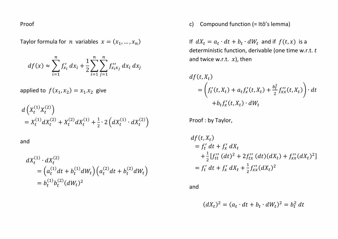
Proof
Taylor formula for � variables � = (��, … , �)
��(�) ≈ � �#G² ��K + 12
K�� � �#G#k²² ��K ��i
i�
K�
applied to �(��, ��) = ��∙�� give
� V��(�)��(�)W
= ��(�)���(�) + ��(�)���(�) + �� ∙ 2 V���(�) ∙ ���(�)W
and
���(�) ∙ ���(�)
= V��(�)�� + ��(�)�)�W V��(�)�� + ��(�)�)�W
= ��(�)��(�)(�)�)�
c) Compound function (= Itô’s lemma)
If ��� = �� ∙ �� + �� ∙ �)� and if �(�, �) is a
deterministic function, derivable (one time w.r.t. �
and twice w.r.t. �), then
��(�, ��)
= ���²(�, ��) + ���#²(�, ��) + ��$� �##²² (�, ��)� ∙ ��
+���#²(�, ��) ∙ �)�
Proof : by Taylor,
��(�, ��)
= ��² �� + �#² ���
+ �� [���²² (��)� + 2��#²² (��)(���) + �##²² (���)�]
= ��² �� + �#² ��� + �� �##²² (���)�
and
(���)� = (�� ∙ �� + �� ∙ �)�)� = ��� ��

Examples
Simple examples
a) ���, �) = �(�)� and �� = )�
�(�(�))�) = �²(�))� �� + �(�) �)�
� �(�(�))�) = �(o))���
= � �²(�))� �� + � �(�) �)�����
� �(�) �)��
� = �(o))� − � �²(�))� ����
(= integration by parts)
b) �(�, �) = �� and �� = )�
�()��) = 12 2 �� + 2)� �)�
� �()��) = )�� = � �� + 2 � )� �)�������
� )� �)��
� = 12 ()�� − o)
c) �(�, �) = ~# and ��� = �� �� + �� �)�
�(~v�) = V�� ~v� + ��$� ~v� W �� + �� ~v� �)�
= ~v� ³V�� + ��$� W �� + �� �)�´
= ~v� ³��� + ��$� ��´
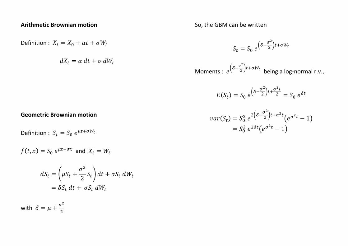
Arithmetic Brownian motion
Definition : �� = �� + z� + &)� ��� = z �� + & �)�
Geometric Brownian motion
Definition : µ� = µ� ~¶�Z���
�(�, �) = µ� ~¶�Z�# and �� = )�
�µ� = �Sµ� + &�2 µ�� �� + &µ� �)�
= ?µ� �� + &µ� �)�
with ? = S + �$�
So, the GBM can be written
µ� = µ� ~��4�$� ��Z���
Moments : ~��4�$$ ��Z���
being a log-normal r.v.,
�(µ�) = µ� ~��4�$� ��Z�$�� = µ� ~��
���(µ�) = µ�� ~���4�$� ��Z�$�F~�$� − 1J
= µ�� ~���F~�$� − 1J

Use of the stochastic differential
Evolution of a financial variable
��� = �� �� + �� �)�
is an equation that describe the evolution of a
financial variable
- For an equity, we have solved the equation :
GBM
- For an option, we will solve it
- For a yield curve, the evolution of a state
variable �� will be describe by a stochastic
differential and we will deduce ·�(0)
However, we will not study the techniques for
solving a general SDE
Classical stochastic differentials in finance
For an Itô stochastic differential, the stochastic
processes ���� and ���� are deterministic
functions of � and ��
Here, these functions do not depend explicitly on
the time variable � �� = ����� �� = �(��)
- Arithmetic Brownian motion ��� = z �� + & �)�
- Geometric Brownian motion ��� = ?�� �� + &�� �)�
- Ornstein-Uhlenbeck process ��� = ?(¸ − ��) �� + & �)�
- Square-root process
��� = ?(¸ − ��) �� + &¹�� �)�

Change of probability measure
- Radon-Nikodym theorem
o Discrete case
o General case
- Girsanov theorem
o Girsanov theorem
o Generalization
Radon-Nikodym theorem
Discrete case
Let Ω = {º�, º�, … , º, … D be the set of
possible outcomes in a random situation with
probability measure Pr :
Pr(BºKD) = »K (∑ »K = 1)
Let E be another probability measure for this
random situation :
E(BºKD) = ¼K (∑ ¼K = 1)
The r.v. ½ is defined by
½(ºK) = ¼K»K

This r.v. has the following properties
- ½ positive
- �¾(½) = ∑ LG¾G »K = 1
- For any r.v. �,
�L(�) = ∑ �(ºK)¼K = ∑ �(ºK) LG¾G »K = �¾(½ ∙ �)
and, in the particular case where � = ¿À,
E(Á) = �¾(½ ∙ ¿À)
General case
Let Pr and E be two probability measures on �Ω, ℱ)
We say that E is absolutely continuous w.r.t. Pr
(E ≪ Pr) if
∀Á ∈ ℱ, E(Á) = 0 ⟹ Pr(Á) = 0
If E ≪ Pr and Pr ≪ E, the two measures are
said equivalent

Radon-Nikodym theorem
E is absolutely continuous w.r.t. Pr
if and only if there exist a positive r.v. ½ such that
∀Á ∈ ℱ, E(Á) = � ½(º) �Pr(º)À
or, equivalently,
E(Á) = �Ä(¿À) = �ÅÆ(½ ∙ ¿À)
½ is named Radon-Nikodym derivative and one
writes
½ = �E�Pr
Property : by putting Á = Ω, we have
1 = E(Ω) = � ½(º) �Pr(º) = �ÅÆ(½)Ç
Girsanov theorem
Girsanov theorem
The definition of a SBM depends heavily on the
probability measure : independent and stationary
increments, normal distribution, …
Let us consider a SBM �)�� on �Ω, ℱ, Pr) for the
time interval [0; o].
The stochastic process F)�J, defined by
)È� = )� + ¼�, is an ABM, but no more a SBM :
�F)È�J = ¼� ≠ 0
The EBM ½� = ~4L��4É$�$ is a positive stochastic
process, martingale, with �¾(½�) = 1. We will use
it as a Radon-Nikodym derivative

Girsanov theorem
• The function
E(Á) = � ½�(º) �Pr(º)À (Á ∈ ℱ)
is a probability measure
• The E measure is equivalent to the Pr
measure
• Under E, F)È�J is a SBM, adapted to the
natural filtration of ()�)
The E measure is the equivalent martingale
measure
Generalization
Let �)�� be a SBM on �Ω, ℱ, Pr) for the time
interval [0; o] and F)�J the associated ABM
with drift S and volatility & :
)� = S� + &)�
Then, F)È�J is an ABM with drift Ê and volatility & under the probability measure
E(Á) = � ½�(º) �Pr(º)À (Á ∈ ℱ)
where
½� = ~Ë4¶�$ �È�4�Ë$4¶$��$ ��


![Bm D% o 9 ] F 0% Bm +f D% Bm D%](https://img.dokumen.tips/doc/110x75/62bed0ece1d6637c2a6a1a76/bm-d-o-9-f-0-bm-f-d-bm-d.jpg)


