Chapter 4: Orthogonal Frequency Division Multiplexing (OFDM)

Jeffrey G. Andrews

March 24, 2006

Orthogonal Frequency Division Multiplexing (OFDM) is a multicarrier modulation technique that has

recently found wide adoption in a wide variety of high data rate communication systems, including Digital

Subscriber Lines (DSL), Wireless LANs (802.11a/g/n), Digital Video Broadcasting, and now, WiMAX and

other emerging wireless broadband systems like Flarion’s proprietary Flash-OFDM and 4G/“Super 3G”

cellular systems. OFDM’s popularity for high-data rate applications stems primarily from its efficient and

flexible management of intersymbol interference (ISI) in highly dispersive channels.

As emphasized in chapter 3, as the channel delay spreadτ becomes an increasingly large multiple of

the symbol timeTs, the ISI becomes very severe. By definition, a high data rate system will generally have

τ � Ts since the number of symbols sent per second is high. In a non-line of sight (NLOS) system such

as WiMAX that must transmit over moderate to long distances, the delay spread will also frequently be

large. In short, wireless broadband systems of all types will suffer from severe ISI, and hence will require

transmitter and/or receiver techniques that overcome the ISI. Although the 802.16 standards include single-

carrier modulation techniques, the vast majority (if not all) 802.16-compliant systems will use the OFDM

modes, which have also been selected as the preferred modes by the WiMAX forum.

This chapter has three main goals to help the WiMAX engineer or student understand how to use OFDM

in a wireless broadband system:

1. Explain the elegance of multicarrier modulation, and how it works in theory.

2. Emphasize a practical understanding of OFDM system design, covering key concepts such as the

cyclic prefix, frequency equalization, synchronization, and channel estimation.

3. Discuss implementation issues for WiMAX systems such as the peak-to-average ratio, and provide

illustrative examples related to WiMAX.

4.1 The Multicarrier Concept

The basic idea of multicarrier modulation is quite simple, and follows naturally from the competing desires

for high data rates and intersymbol interference (ISI) free channels. In order to have a channel that does not

have ISI, the symbol timeTs has to be larger – often significantly larger – than the channel delay spreadτ .

Digital communication systems simply cannot function if ISI is present – an error floor quickly develops

and asTs approaches or falls belowτ , the bit error rate becomes intolerable. As we have noted previously,

for wideband channels that provide the high data rates needed by today’s applications, the desired symbol

time is usually much smaller than the delay spread, so intersymbol interference is severe.

In order to overcome this, multicarrier modulation divides the high-rate transmit bitstream intoL lower-

rate substreams,eachof which hasTs/L >> τ , and is hence ISI-free. These individual substreams can then

be sent overL parallel subchannels, maintaining the total desired data rate. Typically the subchannels are

orthogonal under ideal propagation conditions, in which case multicarrier modulation is often referred to as

orthogonal frequency division multiplexing (OFDM). The data rate on each of the subchannels is much less

than the total data rate, and so the corresponding subchannel bandwidth is much less than the total system

bandwidth. The number of substreams is chosen to insure that each subchannel has a bandwidth less than

1

the coherence bandwidth of the channel, so the subchannels experience relatively flat fading. Thus, the ISI

on each subchannel is small. Moreover, in the digital implementation of OFDM, the ISI can be completely

eliminated through the use of a cyclic prefix.

Example 4.1 A certain wideband wireless channel has a delay spread of1µsec. We assume that in order to

overcome ISI, thatTs ≥ 10τ .

1. What is the maximum bandwidth allowable in this system?

2. If multicarrier modulation is used, and we desire a 5 MHz bandwidth, what is the required number of

subcarriers?

For part (1), if it is assumed thatTs = 10τ in order to satisfy the ISI-free condition, the maximum

bandwidth would be1/Ts = .1/τ = 100 KHz, far below the intended bandwidths for WiMAX systems.

In part (2), if multicarrier modulation is employed, the symbol time goes toT = LTs. The delay spread

criterion mandates that the new symbol time is still bounded to 10% of the delay spread, i.e.(LTs)−1 =100KHz. But the 5 MHz bandwidth requirement gives(Ts)−1 = 5 MHz. Hence,L ≥ 50 allows the full 5

MHz bandwidth to be used with negligible ISI.

4.1.1 An elegant approach to intersymbol interference

Multicarrier modulation in its simplest form divides the wideband incoming data stream intoL narrowband

substreams, each of which is then transmitted over a different orthogonal frequency subchannel. As in

example 4.1, the number of substreamsL is chosen to make the symbol time on each substream much

greater than the delay spread of the channel or, equivalently, to make the substream bandwidth less then the

channel coherence bandwidth. This insures that the substreams will not experience significant ISI.

A simple illustration of a multicarrier transmitter and receiver is given in Figures 4.1 and 4.2. Essentially,

a high-rate data signal of rateR bps and with a passband bandwidthB is broken intoL parallel substreams

each with rateR/L and passband bandwidthB/L. After passing through the channelH(f), the received

signal would appear as shown in 4.3, where we have assumed for simplicity that the pulse-shaping allows

a perfect spectral shaping so that there is no subcarrier overlap1. As long as the number of subcarriers is

sufficiently large to allow for the subcarrier bandwidth to be much less than the coherence bandwidth, i.e.

B/L � Bc, then it can be insured that each subcarrier experiences approximately flat fading. The mutually

orthogonal signals can then be individually detected, as shown in Figure 4.2.

1In practice, there would be some rolloff factor ofβ, so the actual consumed bandwidth of such a system would be(1 + β)B.

However, OFDM as we will see avoids this inefficiency by using a cyclic prefix.

2

S/P

X

X

X

+

cos(2 fc)

cos(2 fc+ f)

cos(2 fc+(L-1) f)

.

.

.

R bps

R/L bps

R/L bps

R/L bpsx(t)

Figure 4.1: A Basic multicarrier transmitter: a high rate stream ofR bps is broken intoL parallel streams

each with rateR/L and then multiplied by a different carrier frequency.

P/S

Demod1

cos(2 fc)

Demod2

DemodL

cos(2 fc+(L-1) f)

.

.

.cos(2 fc+ f)

LPF

LPF

LPF

y(t) R bps

Figure 4.2: A Basic multicarrier receiver: each subcarrier is decoded separately, requiringL independent

receivers.

3

f1 f2 fL

B

Bc

f

|H(f)|

B/L

Figure 4.3: The transmitted multicarrier signal experiences approximately flat fading on each subchannel

sinceB/L � Bc, even though the overall channel experiences frequency selective fading, i.e.B > Bc.

Hence, the multicarrier technique has an interesting interpretation in both the time and frequency do-

mains. In the time domain, the symbol duration on each subcarrier has increased toT = LTs, so by lettingL

grow larger, it can be assured that the symbol duration exceeds the channel delay spread, i.e.T � τ , which

is a requirement for ISI-free communication. In the frequency domain, the subcarriers have bandwidth

B/L � Bc, which assures “flat fading”, the frequency domain equivalent to ISI-free communication.

Although this simple type of multicarrier modulation is easy to understand, it has several crucial short-

comings. First, as noted above, in a realistic implementation, a large bandwidth penalty will be inflicted

since the subcarriers can’t have perfectly rectangular pulse shapes and still be time-limited. Additionally,

very high quality (and hence, expensive) low pass filters will be required to maintain the orthogonality of

the the subcarriers at the receiver. Most importantly, this scheme requiresL independent RF units and

demodulation paths. In Section 4.2, we show how OFDM overcomes these shortcomings.

4.2 OFDM Basics

In order to overcome the daunting requirement forL RF radios in both the transmitter and receiver, OFDM

employs an efficient computational technique known as the Discrete Fourier Transform (DFT), more com-

monly known as the Fast Fourier Transform (FFT)2. In this section, we will learn how the FFT (and its

inverse, the IFFT) are able to create a multitude of orthogonal subcarriers using just a single radio.

2The FFT is a highly efficient implementation of the DFT.

4

4.2.1 Block transmission with guard intervals.

We begin by groupingL data symbols into a block known as anOFDM symbol. An OFDM symbol lasts for

a duration ofT seconds, whereT = LTs. In order to keep each OFDM symbol independent of the others

after going through a wireless channel, it is necessary to introduce a guard time in between each OFDM

symbol, as shown here:

OFDM Symbol OFDM Symbol OFDM Symbolguard guard

This way, after receiving a series of OFDM symbols, as long as the guard timeTg is larger than the delay

spread of the channelτ , each OFDM symbol will only interfere with itself.

OFDM Symbol OFDM Symbol OFDM Symbol

Delay Spread

Put simply, OFDM transmissions allow ISIwithinan OFDM symbol, but by including a sufficiently large

guard band, it is possible to guarantee that there is no interferencebetweensubsequent OFDM symbols.

4.2.2 Circular Convolution and the DFT.

Now that subsequent OFDM symbols have been rendered orthogonal with a guard interval, the next task is

to attempt to remove the ISIwithin each OFDM symbol. As described in Chapter 3, when an input data

streamx[n] is sent through a linear time-invariant FIR channelh[n], the output is the linear convolution of

the input and the channel, i.e.y[n] = x[n] ∗ h[n]. However, let’s imagine for a moment that it was possible

to computey[n] in terms of acircular convolution, i.e.

y[n] = x[n] ~ h[n] = h[n] ~ x[n], (4.1)

where

x[n] ~ h[n] = h[n] ~ x[n] ,L−1∑k=0

h[k]x[n− k]L (4.2)

and the circular functionx[n]L = x[nmodL] is aperiodicversion ofx[n] with periodL. In other words,

each value ofy[n] = h[n] ~ x[n] is the sum of the product ofL terms3.

In this case of circular convolution, it would then be possible to take the DFT of the channel outputy[n]to get:

DFT{y[n]} = DFT{h[n] ~ x[n]} (4.3)

which yields in the frequency domain

Y [m] = H[m]X[m]. (4.4)

3For a more thorough tutorial on circular convolution, the reader is referred to [34] or the “Connexions” web resource

http://cnx.rice.edu/

5

Note that the duality between circular convolution in the time domain and simple multiplication in the

frequency domain is a property unique to the DFT. TheL point DFT is defined as

DFT{x[n]} = X[m] ,1√L

L−1∑n=0

x[n]e−j 2πnmL , (4.5)

while its inverse, the IDFT is defined as

IDFT{X[m]} = x[n] ,1√L

L−1∑m=0

X[m]ej 2πnmL . (4.6)

Referring to (4.4), this innocent formula actually describes an ISI-free channel in the frequency do-

main, where each input symbolX[m] is simply scaled by a complex-valueH[m]. So, given knowledge

of the channel frequency responseH[m] at the receiver, it is trivial to recover the input symbol by simply

computing

X[m] =Y [m]H[m]

, (4.7)

where the estimateX[m] will generally be imperfect due to additive noise, co-channel interference, imper-

fect channel estimation, and other imperfections that will be discussed later. Nevertheless, in principle, the

ISI – which is the most serious form of interference in a wideband channel – has been mitigated.

A natural question to ask at this point is: “where does this circular convolution come from?” After all,

nature provides a linear convolution when a signal is transmitted through a linear channel. The answer is

that this circular convolution can be “faked” by adding a specific prefix called thecyclic prefixonto the

transmitted vector.

4.2.3 The Cyclic Prefix.

The key to making OFDM realizable in practice is the utilization of the FFT algorithm, which has low

complexity. In order for the IFFT/FFT to create an ISI-free channel, the channel must appear to provide a

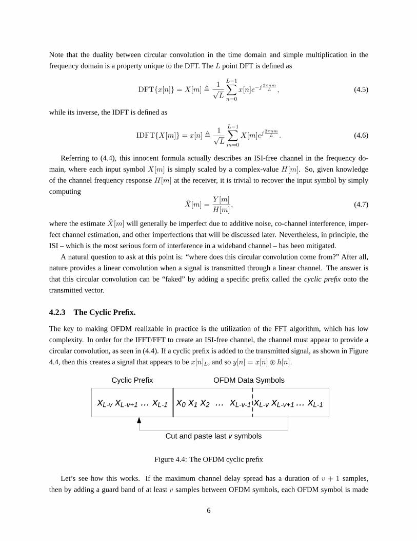
circular convolution, as seen in (4.4). If a cyclic prefix is added to the transmitted signal, as shown in Figure

4.4, then this creates a signal that appears to bex[n]L, and soy[n] = x[n] ~ h[n].

xL-v xL-v+1 ... xL-1 x0 x1 x2 ... xL-v-1 xL-v xL-v+1 ... xL-1

Cyclic Prefix

Cut and paste last v symbols

OFDM Data Symbols

Figure 4.4: The OFDM cyclic prefix

Let’s see how this works. If the maximum channel delay spread has a duration ofv + 1 samples,

then by adding a guard band of at leastv samples between OFDM symbols, each OFDM symbol is made

6

independent of those coming before and after it, and so just a single OFDM symbol can be considered.

Representing such an OFDM symbol in the time domain as a lengthL vector gives

x = [x1 x2 . . . xL]. (4.8)

After applying a cyclic prefix of lengthv, the actual transmitted signal is

xcp = [xL−v xL−v+1 . . . xL−1︸ ︷︷ ︸Cyclic Prefix

x0 x1 . . . xL−1︸ ︷︷ ︸Original data

]. (4.9)

The output of the channel is by definitionycp = h ∗ xcp, whereh is a lengthv + 1 vector describing the

impulse response of the channel during the OFDM symbol4. The outputycp has(L+v)+(v+1)−1 = L+2v

samples. The firstv samples ofycp contain interference from the preceding OFDM symbol, and so are

discarded. The lastv samples disperse into the subsequent OFDM symbol, so also are discarded. This

leaves exactlyL samples for the desired outputy, which is precisely what is required to recover theL data

symbols embedded inx.

Our claim is that theseL samples ofy will be equivalent toy = h ~ x. Various proofs are possible,

the most intuitive is a simple inductive argument. Consider for the moment justy0, i.e. the first element in

y. As shown in Figure 4.5, due to the cyclic prefix,y0 depends onx0 and the circularly wrapped values

xL−v . . . xL−1. That is:

y0 = h0x0 + h1xL−1 + . . . + hvxL−v

y1 = h0x1 + h1x0 + . . . + hvxL−v+1

...

yL−1 = h0xL−1 + h1xL−2 + . . . + hvxL−v−1 (4.10)

From inspecting (4.2), it can be seen that this is exactly the value ofy0, y1, . . . , yL−1 resulting fromy =x ~ h. Thus, by mimicking a circular convolution, a cyclic prefix that is at least as long as the channel

duration allows the channel outputy to be decomposed into a simple multiplication of the channel frequency

responseH = DFT{h} and the channel frequency domain input,X = DFT{x}.The cyclic prefix, although elegant and simple, is not entirely free. It comes with both a bandwidth and

power penalty. Sincev redundant symbols are sent, the required bandwith for OFDM increases fromB toL+v

L B. Similarly, an additionalv symbols must be counted against the transmit power budget. Hence, the

cyclic prefix carries a power penalty of10 log10L+v

L dB in addition to the bandwidth penalty. In summary,

the use of cyclic prefix entails data rate and power losses that are both

Rate Loss = Power Loss =L

L + v.

The “wasted” power has increased importance in an interference-limited wireless system, since it causes

interference to neighboring users. One way to reduce the transmit power penalty is noted in Sidebar 4.1.

4It can generally be reasonably assumed that the channel remains constant over an OFDM symbol, since the OFDM symbol

timeT is usually much less that the channel coherence time,Tc.

7

xL-v xL-v+1 ... xL-1 x0 x1 x2 ... xL-1

hv hv-1 ... h1 h0

y0 = hvxL-v+hv-1xL-v+1 ... +h1xL-1+h0x0

Figure 4.5: The OFDM cyclic prefix creates a circular convolution

It can be noted that forL � v, the inefficiency due to the cyclic prefix can be made arbitrarily small

by increasing the number of subcarriers. However, as the latter parts of this chapter will explain, there

are numerous other important sacrifices that must be made asL grows large. As with most system design

problems, desirable properties such as efficiency must be traded off against cost and required tolerances.

Example 4.2 Referring to Table 9.3, find the minimum and maximum data rate loss due to the cyclic prefix

in WiMAX for a 10 MHz channel with a maximum delay spreadτ = 5µsec.

At a symbol rate of 10 MHz, a delay spread of5µsec affects 50 symbols, so we require a CP length of at

leastv = 50.

The minimum overhead will be for the largest number of subcarriers, referring to Table 9.3 this yields

L = 2048. In this case,v/L = 50/2048 = 1/40.96 so the minimum guard band of1/32 will suffice.

Hence, the data rate loss is only 1/32 in this case.

The maximum overhead occurs when the number of subcarriers is small. IfL = 128, thenv/L =50/128, so even an overhead of1/4 won’t be sufficient to preserve subcarrier orthogonality. More subcar-

riers are required. ForL = 256, v/L < 1/4, so in this case ISI-free operation is possible, but at a data rate

loss of 1/4.

Sidebar 4.1 An Alternative Prefix

8

One alternative to the cyclic prefix is to instead use a “zero prefix”, which as in vector coding constitutes

a null guard band. One commercial system that proposes this is the Intel/Texas Instruments “Multiband

OFDM” system that has been proposed for ultrawideband (UWB) standardization under the context of the

IEEE 802.15.3 subcommittee. As shown in Fig. 4.6 the Multiband OFDM transmitter just sends a prefix of

null data so that there is no transmitter power penalty. At the receiver, the “tail” can be added back in, which

recreates the effect of a cyclic prefix, so the rest of the OFDM system can function as usual.

OFDM Symbol OFDM Symbol OFDM Symbol

Copy Received Tail to front of OFDM Symbol

Send Nothing in Guard Interval

Figure 4.6: The OFDM Zero Prefix allows the circular channel to be recreated at the receiver.

Why wouldn’t every OFDM system use a zero prefix then, since it reduces the transmit power by

10 log10

(L+v

L

)dB? There are two reasons. First, the zero prefix generally increases the receiver power

by 10 log10

(L+v

L

)dB, since the tail now needs to be received (whereas with a cyclic prefix, it can be ig-

nored). Second, additional noise from the received tail symbols is added back into the signal, causing a

higher noise powerσ2 → L+vL σ2. The designer must weigh these tradeoffs to determine whether a zero or

cyclic prefix is preferable. WiMAX systems employ a cyclic prefix.

4.2.4 Frequency Equalization

In order for the received symbols to be estimated, the complex channel gains for each subcarrier must be

known, which corresponds to knowing the amplitude and phase of the subcarrier. For simple modulation

techniques like QPSK that don’t use the amplitude to transmit information, just the phase information is

sufficient.

After the FFT is performed, the data symbols are estimated using a one-tap frequency domain equalizer,

or FEQ, as

Xl =Yl

Hl(4.11)

whereHl is thecomplexresponse of the channel at the frequencyfc + (l − 1)∆f , and therefore it both

corrects the phase and equalizes the amplitude before the decision device. Note that although the FEQ

inverts the channel, there is no problematic noise enhancement or coloring since both the signal and the

noise will have their powers directly scaled by| 1Hl|2.

9

4.2.5 An OFDM Block Diagram

Let us now briefly review the key steps in an OFDM communication system, each of which can be observed

in Figure 4.7.

n

xX L-pt IDFT

L-pt DFT

YP/S Add

CP +h[n] DeleteCP S/P

yFEQ X

Time Domain

Frequency Domain

A circular channel: y = h x + n

Figure 4.7: An OFDM system in vector notation. In OFDM, the encoding and decoding is done in the

frequency domain, whereX, Y, andX contain theL transmitted, received, and estimated data symbols.

1. The first step in OFDM is to break a wideband signal of bandwidthB into L narrowband signals

(subcarriers) each of bandwidthB/L. This way, the aggregate symbol rate is maintained, but each

subcarrier experiences flat-fading, or ISI-free communication. TheL subcarriers for a given OFDM

symbol are represented by a vectorX, which contains theL current symbols.

2. In order to use a single wideband radio instead ofL independent narrow band radios, the subcarriers

are modulated using an IFFT operation.

3. In order for the IFFT/FFT to decompose the ISI channel into orthogonal subcarriers, a cyclic prefix

of lengthv must be appended after the IFFT operation. The resultingL + v symbols are then sent in

serial through the wideband channel.

4. At the receiver, the cyclic prefix is discarded, and theL received symbols are demodulated using an

FFT operation, which results inL data symbols, each of the formYl = HlXl + Nl for subcarrierl.

5. Each subcarrier can then be equalized via an FEQ by simply dividing by the complex channel gain

H[i] for that subcarrier. This results inXl = Xl + Nl/Hl.

We have neglected a number of important practical issues thus far. For example, we have assumed that

the transmitter and receiver are perfectly synchronized, and that the receiver perfectly knows the channel

(in order to perform the FEQ). In the next section, we overview the implementation issues for OFDM in

WiMAX.

10

4.3 An Example: OFDM in WiMAX

To gain an appreciation for the time and frequency domain interpretations of OFDM, WiMAX systems can

be used as an example. Although simple in concept, the subtleties of OFDM can be confusing if each signal

processing step is not understood. To ground the discussion, we will consider a passband OFDM system,

and then give specific values for the important system parameters.

Figure 4.8 shows an up close view of a passband OFDM modulation engine. The inputs to this figure

areL independent QAM symbols (the vectorX), and theseL symbols are treated as separate subcarriers.

TheseL data-bearing symbols can be created from a bit stream by a symbol mapper and serial-to-parallel

convertor (S/P). TheL-point IFFT then creates a time domainL-vectorx that is cyclic extended to have

lengthL(1 + G), whereG is the fractional overhead. This longer vector is then parallel-to-serial (P/S)

converted into a wideband digital signal that can be amplitude modulated with a single radio at a carrier

frequency offc = ωc/2π.

IFFT

P/S

Speed = B/L HzL Subcarriers

Speed = B/L HzL(1+G) Samples

Serial Stream atB(1+G) Hz

Cyclic Prefix ofLG Samples

QAM Symbols

(X)

D/A X

Analog BasebandMulticarrier

Signal

RFMulticarrier

Signal

exp(j c)

Figure 4.8: A closeup of the OFDM baseband transmitter.

This procedure appears to be relatively straightforward, but in order to be a bit less abstract, we will

now use some plausible values for the different parameters. Chapter 9 enumerates all the legal values for

the OFDM parametersB, L, Lg, andG. The key OFDM parameters are summarized in Table 4.1, along

with some potential numerical values for these parameters. As an example, if 16QAM modulation was used

(M = 16), the raw (neglecting coding) data rate of this WiMAX system would be:

R =B

L

Ld log2(M)1 + G

(4.12)

=107MHz

1024768 log2(16)

1.125= 24Mbps. (4.13)

In words, there areLd data-carrying subcarriers of bandwidthB/L, each carryinglog2(M) bits of data.

An additional overhead penalty of(1 + G) must be paid for the cyclic prefix, since it consists of redundant

information and sacrifices the transmission of actual data symbols.

11

Table 4.1: Summary of OFDM Parameters. WiMAX specified parameters are denoted by an asterisk (∗):the other OFDM parameters can all be derived from these values.Symbol Description Relation Example WiMAX value

B∗ Nominal bandwidth B = 1/Ts 10 MHz

L∗ No. of subcarriers size of IFFT/FFT 1024

G∗ Guard fraction % of L for CP 1/8

Lg∗ Data subcarriers L− pilot/null subcarriers 768

Ts Sample time Ts = 1/B 1 µsec

Ng Guard symbols Ng = GL 128

Tg Guard time Tg = TsNg 12.8µsec

T OFDM symbol time T = Ts(L + Ng) 115.2µsec

Bsc Subcarrier Bandwidth Bsc = B/L 9.76 KHz

4.4 Timing and Frequency Synchronization

In order to demodulate an OFDM signal, there are two important synchronization tasks that need to be

performed by the receiver. First, the timing offset of the symbol and the optimal timing instants need to

be determined. This is referred to astiming synchronization. Second, the receiver must align its carrier

frequency as closely as possible with the transmitted carrier frequency. This is referred to asfrequency

synchronization. Compared to single-carrier systems, the timing synchronization requirements for OFDM

are in fact somewhat relaxed, since the OFDM symbol structure naturally accommodates a reasonable degree

of synchronization error. On the other hand, frequency synchronization requirements are significantly more

stringent, since the orthogonality of the data symbols is reliant on their being individually discernible in the

frequency domain.

Figure 4.9 shows a representation of an OFDM symbol in time (left) and frequency (right). In the time

domain, the IFFT effectively modulates each data symbol onto a unique carrier frequency. In Figure 4.9

only two of the carriers are shown – the actual transmitted signal is the superposition of all the individual

carriers. Since the time window isT = 1µsec and a rectangular window is used, the frequency response of

each subcarrier becomes a “sinc” function with zero crossings every1/T = 1 MHz. This can be confirmed

using the Fourier TransformF{·} since

F{cos(2πfc) · rect(t/T )} = F{cos(2πfc)} ∗ F{rect(2t/T )} (4.14)

= sinc (T (f − fc)) , (4.15)

whererect(x) = 1, x ∈ (−0.5, 0.5), and zero elsewhere. This frequency response is shown forL = 8subcarriers in the right of Figure 4.9.

The challenge of timing and frequency synchronization can be appreciated by inspecting these two

figures. If the timing window is slid to the left or right, a unique phase change will be introduced to each

of the subcarriers. In the frequency domain, if the carrier frequency synchronization is perfect, the receiver

samples at the peak of each subcarrier, where the desired subcarrier amplitude is maximized and the inter-

12

0 0.1 0.2 0.3 0.4 0.5 0.6 0.7 0.8 0.9 1−1.5

−1

−0.5

0

0.5

1

1.5

Time (µsec)

cos(2πfct)

cos(2π(fc + ∆ f)t)

8 9 10 11 12 13 14 15 16 17 18 19−0.5

0

0.5

1

1.5

Frequency (MHz)

perfectsynch.

imperfect synch

δ

Figure 4.9: OFDM synchronization in time (left) and frequency (right). Here, two subcarriers in the time

domain and eight subcarriers in the frequency domain are shown, wherefc = 10 MHz and the subcarrier

spacing∆f = 1 Hz.

carrier interference (ICI) is zero. However, if the carrier frequency is misaligned by some amountδ, then

some of the desired energy is lost, and more significantly, inter-carrier interference is introduced.

The following two subsections will more carefully examine timing and frequency synchronization. Al-

though the development of good timing and frequency synchronization algorithms for WiMAX systems is

the responsibility of each equipment manufacturer, we will give some general guidelines on what is required

of a synchronization algorithm, and discuss the penalty for imperfect synchronization. It should be noted that

synchronization is one of the most challenging problems in OFDM implementation, and the development of

efficient and accurate synchronization algorithms presents an opportunity for technical differentiation and

intellectual property.

4.4.1 Timing Synchronization

The effect of timing errors in symbol synchronization is somewhat relaxed in OFDM due to the presence

of a cyclic prefix. In Section 4.2.3, we assumed that only theL time domain samples after the cyclic prefix

were utilized by the receiver. Indeed, this corresponds to “perfect” timing synchronization, and in this case

even if the cyclic prefix lengthNg is equivalent to the length of the channel impulse responsev, successive

OFDM symbols can be decoded ISI free.

In the case that perfect synchronization is not maintained, it is still possible to tolerate a timing offset

of τ seconds without any degradation in performance as long as0 ≤ τ ≤ Tm − Tg, where as usualTg

is the guard time (cyclic prefix duration) andTm is the maximum channel delay spread. Here,τ < 0corresponds to sampling earlier than at the ideal instant, whereasτ > 0 is later than the ideal instant. As

long as0 ≤ τ ≤ Tm − Tg, the timing offset can be included by the channel estimator in the complex gain

estimate for each subchannel and the appropriate phase shift can be applied by the FEQ without any loss

in performance – at least in theory. This acceptable range ofτ is referred to as the timing synchronization

13

margin, and is shown in Figure 4.10.

On the other hand, if the timing offsetτ is not within this window0 ≤ τ ≤ Tm − Tg, inter-symbol

interference (ISI) occurs regardless of whether the phase shift is appropriately accounted for. This can be

confirmed intuitively for the scenario thatτ > 0 and forτ < Tm − Tg. For the caseτ > 0, the receiver

loses some of the desired energy (since only delayed version of the early samplesx0, x1, ... are received),

and also incorporates undesired energy from the subsequent symbol. Similarly forτ < Tm − Tg, desired

energy is lost while interference from the preceding symbol is included in the receive window. For both of

these scenarios, the SNR loss can be approximated by

∆SNR(τ) ≈ −2(

τ

LTs

)2

, (4.16)

which makes intuitive sense given the above arguments, and has been shown more rigorously in the literature

on synchronization for OFDM. Important observations from this expression are that:

1. SNR decreases quadratically with the timing offset

2. Longer OFDM symbols are increasingly immune from timing offset, i.e. more subcarriers helps.

3. Since in generalτ � LTs, timing synchronization errors are not that critical as long as the induced

phase change is corrected.

In summary, to minimize SNR loss due to imperfect timing synchronization, the timing errors should be

kept small compared to the guard interval, and a small margin in the cyclic prefix length is helpful.

CP CP L Data SymbolsL Data Symbols

Delay Spread (v samples, Tm secs)

Synch. Margin (Ng – v samples, Tg – Tm secs)

Figure 4.10:

4.4.2 Frequency Synchronization

OFDM achieves a high degree of bandwidth efficiency compared to other wideband systems. The subcarrier

packing is extremely tight compared to conventional modulation techniques which require a guard band on

the order of 50% or more, in addition to special transmitter architectures such as the Weaver architecture or

Single-Sideband modulation that suppress the redundant negative-frequency portion of the passband signal.

The price to be paid for this bandwidth efficiency is that the multicarrier signal shown in Figure 4.9 is very

sensitive to frequency offsets due to the fact that the subcarriers overlap, rather than having each subcarrier

truly spectrally isolated.

14

Since the zero crossings of the frequency domain sinc pulses all line up as seen in Figure 4.9, as long as

the frequency offsetδ = 0, there is no interference between the subcarriers. One intuitive interpretation for

this is that since the FFT is essentially a frequency sampling operation, if the frequency offset is negligible

the receiver simply samplesy at the peak points of the sinc functions, where the ICI is zero from all the

neighboring subcarriers.

In practice, of course, the frequency offset is not always zero. The major causes for this are mismatched

oscillators at the transmitter and receiver and Doppler frequency shifts due to mobility. Since precise crystal

oscillators are expensive, tolerating some degree of frequency offset is essential in a consumer OFDM

system like WiMAX. For example, if an oscillator is accurate to0.1 parts per million (ppm),foffset ≈(fc)(0.1ppm). If fc = 3 GHz and the Doppler is 100 Hz, thenfoffset = 300 + 100 Hz, which will

degrade the orthogonality of the received signal, since now the received samples of the FFT will contain

interference from the adjacent subcarriers. We’ll now analyze this intercarrier interference (ICI) in order to

better understand its effect on OFDM performance.

The matched filter receiver corresponding to subcarrierl can be simply expressed for the case of rectan-

gular windows (neglecting the carrier frequency) as

xl(t) = Xlej 2πlt

LTs , (4.17)

where1/LTs = ∆f , and againLTs is the duration of the data portion of the OFDM symbol, i.e.T =Tg + LTs. An interfering subcarrierm can be written as

xl+m(t) = Xmej2π(l+m)t

LTs . (4.18)

If the signal is demodulated with a fractional frequency offset ofδ, |δ| ≤ 12

xl+m(t) = Xmej2π(l+m+δ)t

LTs . (4.19)

The ICI between subcarriersl andl + m using a matched filter (i.e. the FFT) is simply the inner product

between them:

Im =

LTs∫0

xl(t)xl+m(t)dt =LTsXm

(1− e−j2π(δ+m)

)j2π(m + δ)

. (4.20)

It can be seen that in the above expression,δ = 0 ⇒ Im = 0, andm = 0 ⇒ Im = 0, as expected. The total

average ICI energy per symbol on subcarrierl is then

ICIl = E[∑m6=l

|Im|2] ≈ C0(LTsδ)2Ex, (4.21)

whereC0 is a constant that depends of various assumptions andEx is the average symbol energy [36, 27].

The approximation sign is due to the fact that this expression assumes that there are an infinite number of

interfering subcarriers. Since the interference falls off quickly withm, this assumption is very accurate for

subcarriers near the middle of the band, and is pessimistic by a factor of 2 for at either end of the band.

15

SNR = 20 dB SNR = 10 dB

SNR = 0 dB

0.001

0.01

0.1

1

10

0 0.01 0.02 0.03 0.04 0.05

Relative Frequency Offset, δ

SNR

Deg

rada

tion

in d

B

Figure 4.11: SNR loss as a function of the relative frequency offsetδ. The solid lines are for a fading channel

and the dotted lines are for an AWGN channel.

The SNR loss induced by frequency offset is given by

∆SNR =Ex/No

Ex/(No + C0(LTsδ)2Ex)(4.22)

= 1 + C0(LTsδ)2SNR (4.23)

Important observations from the ICI expression (4.23) and Figure 4.11 are that:

1. SNR decreases quadratically with the frequency offset

2. SNR decreases quadratically with the number of subcarriers.

3. The loss in SNR is also proportional to the SNR itself.

4. In order to keep the loss negligible, say less than 0.1 dB, the frequency offset needs to be in the 1-2%

range, or even lower to preserve high SNRs.

5. Therefore, this is a case where reducing the CP overhead by increasing the number of subcarriers

causes an offsetting penalty, introducing a tradeoff.

In order to further reduce the ICI for a given choice ofL, non-rectangular windows can also be used

[30, 37].

4.4.3 Obtaining Synchronization in WiMAX

The preceding two sections discussed the consequences of imperfect time and frequency synchronization.

There have been many synchronization algorithms developed in the literature, a by no means exhaustive list

includes [39, 6, 42, 28, 16]. Generally, the proposed can be broken into the following two categories:

16

Pilot symbol based. In this class, known pilot symbols are transmitted. Since the receiver knows

what was transmitted, attaining quick and accurate time and frequency synchronization is the easiest in this

case, at the cost of surrendering some throughput. In the WiMAX downlink, the preamble consists of a

known OFDM symbol that can be used to attain initial synchronization. In the WiMAX uplink, the periodic

ranging (described in Chapter 9) can be used to synchronize. Since WiMAX is an OFDMA system with

many competing users, each user implements the synchronization at the mobile. This requires the base

station to communicate the frequency offset to the SS.

Blind, or Cyclic prefix based. “Blind” means that pilot symbols are not available to the receiver, so

the receiver must do the best it can without explicitly being able to determine the effect of the channel. In

the absence of pilot symbols, the cyclic prefix, which contains redundancy, can also be used to attain time

and frequency synchronization [39]. This technique is effective when the number of subcarriers is large, or

when the offsets are estimated over a number of consecutive symbols. The principle benefit of CP-based

methods are that pilot symbols are not needed, so the data rate can nominally be increased. In WiMAX,

accurate synchronization and especially channel estimation are considered important enough to warrant the

use of pilot symbols, so the blind techniques are not usually used for synchronization. They could be used

to track the channel in between preambles or ranging signals, but the frequency and timing offsets generally

vary slowly enough that this is not required.

4.5 Channel Estimation in OFDM

TBD. This may just get covered in the Chapter 6 section on MIMO-OFDM channel estimation, since OFDM

is just a special case of that.

4.6 The Peak to Average Ratio

OFDM signals have a higher Peak-to-Average Ratio (PAR) – often called a Peak-to-Average Power Ratio

(PAPR) – than single carrier signals. The reason for this is that in the time domain, a multicarrier signal is

the sum of many narrowband signals. At some time instances, this sum is large, at other times it is small,

which means that the peak value of the signal is substantially larger than the average value. This high PAR

is one of the most important implementation challenges that faces OFDM because it reduces the efficiency

and hence increases the cost of the RF power amplifier, which is one of the most expensive components in

the radio. In this section, we will quantify the PAR problem, explain its severity in WiMAX, and briefly

overview some strategies for reducing the PAR.

4.6.1 The PAR Problem

When a high peak signal is transmitted through a nonlinear device such as a high power amplifier (HPA) or

digital-to-analog converter (DAC), it generates out-of-band energy (spectral regrowth) and in-band distortion

(constellation tilting and scattering). These degradations may affect the system performance severely. The

nonlinear behavior of HPA can be characterized by amplitude modulation-amplitude modulation (AM/AM)

17

and amplitude modulation-phase modulation (AM/PM) responses. Figure 4.12 shows a typical AM/AM

response for a HPA, with the associated input and output back off regions; IBO and OBO, respectively.

Vout

Vin

Linear Region

Nonlinear Region

Avg Peak

IBO

OB

O

Figure 4.12: A typical power amplifier response. Operation in the linear region is required in order to avoid

distortion, so the peak value must be constrained to be in this region, which means that on average, the

power amplifier is underutilized by a “backoff” amount.

To avoid the undesirable nonlinear effects just mentioned, a waveform with high peak power must be

transmitted in the linear region of the HPA by decreasing the average power of the input signal. This is called

(input) backoff (IBO) and results in a proportional output backoff (OBO). High backoff reduces the power

efficiency of the HPA, and may limit the battery life for mobile applications. In addition to inefficiency in

terms of power, the coverage range is reduced and the cost of the HPA is higher than would be mandated by

the average power requirements.

The input backoff is defined as

IBO = 10 log10

PinSat

Pin, (4.24)

wherePinSat is the saturation power (above which is the nonlinear region) andPin is the average input

power. The amount of backoff is usually greater than or equal to the PAR of the signal.

The power efficiency of a HPA can be increased by reducing the PAR of the transmitted signal. For

example, the efficiency of a class A amplifier is halved when the input PAR is doubled or the operating point

(average power) is halved [13, 5]. The theoretical efficiency limits for two classes of HPAs are shown in

Fig. 4.13. Clearly, it would be desirable to have the average and peak values be as close together as possible

in order to maximize the efficiency of the power amplifier.

In addition to the large burden placed on the HPA, a high PAR requires high resolution for both the

transmitter’s digital-to-analog convertor (DAC) and the receiver’s analog-to-digital convertor (ADC), since

the dynamic range of the signal is proportional to the PAR. High resolution D/A and A/D conversion places

an additional complexity, cost, and power burden on the system.

18

0 2 4 6 8 10 12 140

20

40

60

80

100

Peak-to-Average Power Ratio(dB)

Effic

ienc

y (%

)

Class AClass B

Figure 4.13: Theoretical efficiency limits of linear amplifiers [26]. A typical OFDM PAR is in the 10 dB

range, so the PA efficiency is 50-75% lower than in a single carrier system.

4.6.2 Quantifying the PAR

Since multicarrier systems transmit data over a number of parallel frequency channels, the resulting wave-

form is the superposition ofL narrowband signals. In particular, each of theL output samples from aL-pt

IFFT operation involves the sum ofL complex numbers, as can be seen from (4.6). Due to the Central Limit

Theorem, the resulting output values{x1, x2, . . . , xL} can be accurately modelled (particularly for largeL)

as complex Gaussian random variables with zero mean and varianceσ2 = Ex/2, i.e. the real and imaginary

parts both have zero mean and varianceσ2 = Ex/2. The amplitude of the output signal is

|x[n]| =√

(Re{x[n]})2 + (Im{x[n]})2, (4.25)

which is Rayleigh distributed with parameterσ2. The output power is therefore

|x[n]|2 = (Re{x[n]})2 + (Im{x[n]})2, (4.26)

which is exponentially distributed with mean2σ2. The important thing to note is that the output amplitude

and hence power arerandom, so the PAR is not a deterministic quantity either.

The PAR of the transmitted analog signal can be defined as

PAR ,max

t|x(t)|2

E[|x(t)|2], (4.27)

where naturally the range of time to be considered has to be bounded over some interval. Generally, the

PAR is considered for a single OFDM symbol, which consists ofL + Ng samples, or a time duration ofT ,

19

as this chapter has explained. Similarly, the discrete-time PAR can be defined for the IFFT output as

PAR ,

maxl∈(0,L+Ng)

|xl|2

E[|xl|2]=Emax

Ex. (4.28)

It is important to recognize, however, that although the average energy of IFFT outputsx[n] is the same as

the average energy of the inputsX[m] and equal toEx, the analog PAR isnot generally the same as the

PAR of the IFFT samples, due to the interpolation performed by the D/A convertor. Usually, the analog

PAR is higher than the digital (Nyquist sampled) PAR. Since the PA is by definition analog, the analog PAR

is what determines the PA performance. Similarly, DSP techniques developed to reduce the digital PAR

may not always have the anticipated effect on the analog PAR, which is what matters. In order to bring the

analog PAR expression in (4.27) and the digital PAR expression in (4.28) closer together, oversampling can

be considered for the digital signal. That is, a factorM additional samples can be used to interpolate the

digital signal in order to better approximate its analog PAR.

It can be proven that the maximum possible value of the PAR isL, which occurs when all the subcarriers

add up constructively at a single point. However, although it is possible to choose an input sequence that

results in this very high PAR, such an expression for PAR is misleading. For independent binary inputs, for

example, the probability of this maximum peak value occurring is on the order of2−L.

Since the theoretical maximum (or similar) PAR value seldom occurs, a statistical description of the PAR

is commonly used. The complementary cumulative distribution function (CCDF = 1 - CDF) of the PAR is

the most commonly used measure. The distribution of the OFDM PAR has been studied by many researchers

[43, 32, 31, 3]. Among these, van Nee and de Wild introduced a simple and accurate approximation of the

CCDF for largeL(≥ 64):

CCDF(L, Emax) = 1−G(L, Emax) = 1− F (L, Emax)βL = 1−(

1− exp(Emax

2σ2))βL

, (4.29)

whereEmax is the peak power level andβ is a pseudo-approximation of the oversampling factor which is

given empirically asβ = 2.8 [43]. Note that the PAR isEmax/2σ2 andF (L, Emax) is the CDF of a single

Rayleigh distributed subcarrier with parameterσ2. The basic idea behind this approximation is that unlike

a Nyquist5 sampled signal, the samples of an oversampled OFDM signal are correlated, making it hard to

derive an exact peak distribution. The CDF of the Nyquist sampled signal power can be obtained by

G(L, Emax) = P (max ||x(t)|| ≤ Emax) = F (L, Emax)L, (4.30)

Using this result as a baseline, the oversampled case can be approximated in a heuristic way by regarding

the oversampled signal as generated byβL Nyquist sampled subcarriers. Note however thatβ is not equal to

the oversampling factorM . This simple expression is quite effective for generating accurate PAR statistics

for various scenarios, and sample results are displayed in Figure 4.14. As expected, the approximation is

accurate for largeL and the PAR of OFDM system increases withL but not nearly linearly.

5Nyquist sampling means the minimum allowable sampling frequency without irreversible information loss, i.e. no oversam-

pling is performed.

20

2 4 6 8 10 12 1410

−5

10−4

10−3

10−2

10−1

100

PAR(dB)

CC

DF

L = 16

L = 64

L = 256

L = 1024

Figure 4.14: CCDF of PAR for QPSK OFDM system:L = 16, 64, 256, 1024. Solid line: simulation results,

dotted line: approximation usingβ = 2.8.

4.6.3 Clipping: Living with a High PAR

In order to avoid operating the PA in the nonlinear region, the input power can be reduced by an amount

about equal to the PAR. However, two important facts related to this IBO amount can be observed from

Figure 4.14. First, since the highest PAR values are uncommon, it might be possible to simply “clip” off the

highest peaks in order to reduce the IBO and effective PAR, at the cost of some hopefully minimal distortion

of the signal. Second and conversely, it can be seen that even for a conservative choice of IBO, say 10dB,

there is still a distinct possibility that a given OFDM symbol will have a PAR that exceeds the IBO and

causes clipping.

Clipping, sometimes called “soft limiting”, truncates the amplitude of signals that exceed the clipping

level as

xL[n] =

Aej∠x[n], if |x[n]| > A

x[n], if |x[n]| ≤ A,(4.31)

wherex[n] is the original signal, andx[n] is the output after clipping. The soft limiter can be equivalently

thought of as a peak cancellation technique, like that shown in Figure 4.15. The soft limiter output can be

written in terms of the original signal and a cancelling, or “clipping signal” as

x[n] = x[n] + c[n], for n = 0, . . . , L− 1 (4.32)

wherec[n] is the clipping signal defined by

c[n] =

{|A− |x[n]||ejθ[n], if |x[n]| > A

0, if |x[n]| ≤ Afor n = 0, ..., NL− 1 (4.33)

21

Anti-peakGenerator

+

][nc

][nx ][nx

dB5=γ

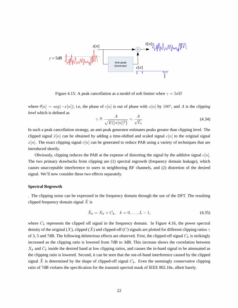
Figure 4.15: A peak cancellation as a model of soft limiter whenγ = 5dB

whereθ[n] = arg(−x[n]); i.e, the phase ofc[n] is out of phase withx[n] by 180o, andA is theclipping

levelwhich is defined as

γ ,A√

E{|x[n]|2}=

A√Ex

(4.34)

In such a peak cancellation strategy, an anti-peak generator estimates peaks greater than clipping level. The

clipped signalx[n] can be obtained by adding a time-shifted and scaled signalc[n] to the original signal

x[n]. The exact clipping signalc[n] can be generated to reduce PAR using a variety of techniques that are

introduced shortly.

Obviously, clipping reduces the PAR at the expense of distorting the signal by the additive signalc[n].The two primary drawbacks from clipping are (1) spectral regrowth (frequency domain leakage), which

causes unacceptable interference to users in neighboring RF channels, and (2) distortion of the desired

signal. We’ll now consider these two effects separately.

Spectral Regrowth

. The clipping noise can be expressed in the frequency domain through the use of the DFT. The resulting

clipped frequency domain signalX is

Xk = Xk + Ck, k = 0, . . . , L− 1, (4.35)

whereCk represents the clipped off signal in the frequency domain. In Figure 4.16, the power spectral

density of the original (X), clipped (X) and clipped-off (C) signals are plotted for different clipping ratiosγ

of 3, 5 and 7dB. The following deleterious effects are observed. First, the clipped-off signalCk is strikingly

increased as the clipping ratio is lowered from 7dB to 3dB. This increase shows the correlation between

Xk andCk inside the desired band at low clipping ratios, and causes the in-band signal to be attenuated as

the clipping ratio is lowered. Second, it can be seen that the out-of-band interference caused by the clipped

signalX is determined by the shape of clipped-off signalCk. Even the seemingly conservative clipping

ratio of 7dB violates the specification for the transmit spectral mask of IEEE 802.16e, albeit barely.

22

0 0.1 0.2 0.3 0.4 0.5 0.6 0.7 0.8 0.9 1-60

-50

-40

-30

-20

-10

0

10

Normalized frequency

PSD

(dB

)

orginal signal clipped-off signal clipped signal

:X:C:~X

dB3~7=γ

dB3=γ

dB5=γ

dB7=γ

Spectral Mask

Figure 4.16: Power Spectral Density of the unclipped (original) and clipped (nonlinearly distorted) OFDM

signals with 2048 block size and 64 QAM when clipping ratio (γ) is 3, 5, and 7dB in soft limiter.

In-band Distortion

. Although the desired signal and the clipping signal are clearly correlated, it is possible based on the Buss-

gang Theorem to model the in-band distortion due to the clipping process as the combination of uncorrelated

additive noise and an attenuation of the desired signal [15, 14, 33]:

x[n] = αx[n] + d[n], for n = 0, 1, . . . , L− 1. (4.36)

Now, d[n] is uncorrelated with the signalx[n] and the attenuation factorα is obtained by

α = 1− e−γ2+√

πγ

2erfc(γ). (4.37)

The attenuation factorα is plotted in Figure 4.17 as a function of the clipping ratioγ. The attenuation

factorα is negligible when the clipping ratioγ is greater than 8dB, so high clipping ratios, the correlated

clipped-off signalc[n] in (4.33) can be approximated by uncorrelated noised[n]. That is,c[n] ≈ d[n] asγ ↑.The variance of the uncorrelated clipping noise can be expressed assuming a stationary Gaussian inputx[n]as

σ2d = Ex(1− exp(−γ2)− α2). (4.38)

In WiMAX, the error vector magnitude (EVM) is used as a means to estimate the accuracy of the

transmit filter and D/A converter as well as the PA non-linearity. The EVM is essentially the average error

23

0 2 4 6 8 10 120.75

0.8

0.85

0.9

0.95

1

Clipping ratio γ (dB)

Atte

nuat

ion

fact

or α

Figure 4.17: Attenuation factorα as a function of the clipping ratioγ

vector relative to the desired constellation point, and can be caused by an degradation in the system. The

EVM over an OFDM symbol is defined as

EVM =

√1N

∑Lk=1(∆I2

k + ∆Q2k)

S2max

=

√σ2

d

S2max

(4.39)

whereSmax the maximum constellation amplitude. The concept of EVM is visually illustrated in Figure

4.18. In the case of clipping, a given EVM specification can be easily translated into an SNR requirement

using the varianceσ2d of the clipping noise.

It is possible to define the signal-to-noise-plus-distortion ratio (SNDR) of one OFDM symbol in order

to estimate the impact of clipped OFDM signals over an AWGN channel under the assumption that the

distortiond[n] is Gaussian and uncorrelated with the input and channel noise (that has varianceN0/2):

SNDR=α2Ex

σ2d + N0/2

. (4.40)

The bit-error probability (BEP) can be evaluated for different modulation types using the SNDR [14]. In the

case of M-QAM and average powerEx, the BEP can then be approximated as

Pb ≈4

log2 M

(1− 1√

M

)Q

(√3Exα2

(σ2d + N0/2)(M − 1)

). (4.41)

Figure 4.19 shows the BER for an OFDM system with L = 2048 subcarriers and 64-QAM modulation. As

the SNR increases, the clipping error dominates the additive noise and an error floor is observed. The error

floor can be inferred from (4.41) by letting the noise varianceN0/2 → 0.

A number of additional studies of clipping in OFDM systems have been completed in recent years, e.g.

[38, 14, 4, 3, 31]. In some cases clipping may be acceptable, but in WiMAX systems the margin for error

24

Imag

inar

yReference

Signal

MeasuredSignal

Error Vector

Figure 4.18: Illustrative example of EVM

is quite tight, as much of this book has emphasized. Hence, more aggressive and innovative techniques

for reducing the PAR are being actively pursued by the WiMAX community in order to bring down the

component cost and to reduce the degradation due to the nonlinear effects of the PA.

4.6.4 PAR Reduction Strategies

To alleviate the nonlinear effects mentioned above, numerous approaches have been pursued. The first

plan of attach is to reduce PAR at the transmitter, either through peak cancellation or signal mapping [20].

Another set of techniques focuses on OFDM signal reconstruction at the receiver in spite of the introduced

nonlinearities, e.g. [23, 41]. A further approach is to attempt to predistort the analog signal so that it will

appear to have been linearly amplified [8]. In this section, we will overview techniques that attempt PAR

reduction at the transmitter.

Peak Cancellation

This class of PAR reduction techniques applies an anti-peak signal to the desired signal. Although clipping

is the most obvious such technique, and was discussed in detail in the last section, other important peak

cancelling techniques include tone reservation (TR) and active constellation extension (ACE).

Clipping can be improved by an iterative clipping and filtering process, since the filtering can be used

to subdue the spectral regrowth and in band distortion [2]. After several iterations of clipping and filtering,

the residual in-band distortion can be restored by iterative estimation and cancellation of the clipping noise

[9].

25

5 10 15 20 25 30

10-6

10-4

10-2

100

Eb/No (dB)

Bit

erro

r rat

e : P

b

γ = 3dBγ = 4dBγ = 5dBγ = 6dBγ = 7dBγ = ∞

Figure 4.19: Bit error rate probability for a clipped OFDM signal in AWGN with different clipping ratios.

Tone reservation reduces PAR by intelligently adding power to unused carriers, such as the null subcar-

riers specified by WiMAX. The reduced signal can be expressed as

x[n] = x[n] + c[n] = QL(X + C) (4.42)

whereQL is the IDFT matrix of sizeL×L, X = {Xk, k ∈ Rc} is complex symbol vector,C = {Ck, k ∈ R}is a complex tone reservation vector, andR is the reserved tones set. There is no distortion from TR because

the reserved tone carriers and the data carriers are orthogonal. To reduce PAR using TR, a simple gradient

algorithm and a Fourier projection algorithm have been proposed in [40] and [18], respectively. However,

these technique converge slowly. For faster convergence, an active set approach is used in [25].

Another peak cancelling technique is active constellation extension (ACE) [24]. Essentially, the corner

points of an M-QAM constellation can be extended without any loss of SNR, and this property can be used

to decrease the PAR without negatively effecting the performance as long as ACE be allowed only in the case

that the minimum distance is guaranteed. Unfortunately, the gain in PAR reduction is inversely proportional

to the constellation size in M-QAM.

Signal Mapping

Signal mapping techniques share in common that some redundant information is added to the transmitted

signal in a manner which reduces the PAR. This class includes coding techniques, selected mapping (SLM),

and partial transmit sequence (PTS).

26

The main idea behind the various coding schemes is to select a low PAR codeword based on the desired

transmit symbols [22, 35]. However, most of the decoding techniques for these codes require an exhaustive

search so are feasible only for a small number of subcarriers. Moreover, it is difficult to maintain a reasonable

coding rate in OFDM when the number of subcarriers grows large. The implementation prospects for the

coding-based techniques appear dim.

In Selected mapping, one OFDM symbol is used to generate multiple representations that have the same

information as the original symbol [29]. The basic objective is to select the one with minimum PAR, and

the gain in PAR reduction is proportional to the number of the candidate symbols, but so is the complexity.

PTS is similar to SLM; however, the symbol in the frequency domain is partitioned into smaller disjoint

subblocks. The objective is to design an optimal phase for the subblock set that minimizes the PAR. The

phase can then be corrected at the receiver. The PAR reduction gain depends on the number of subblocks and

the partitioning method. However, PTS has exponential search complexity with the number of subblocks.

SLM and PTS are quite flexible and effective, but their principle drawbacks are that the receiver structure

must be changed and transmit overhead (power and symbols) are required to send the needed information

for decoding. Hence, these techniques, in contrast to peak cancellation techniques, would require explicit

support by the WiMAX standard.

4.7 The Computational Complexity Advantage of OFDM

One of the principal advantages of OFDM relative to single carrier modulation with equalization is that

it requires much lower computational complexity for high data rate communication. In this section we

compare the computational complexity of an equalizer with that of a standard IFFT/FFT implementation of

OFDM.

An equalizer operation consists of a series of multiplications with several delayed versions of the signal.

The number of delay taps in an equalizer depends on the symbol rate of the system and the delay spread

in the channel. To be more precise, the number of equalizer taps is proportional to the bandwidth-delay

spread productTm/Ts ≈ BTm. We have been calling this quantityv, or the number of ISI channel taps.

An equalizer withv taps performsv complex multiply and accumulate (CMAC) operations per received

symbol. Therefore, the complexity of an equalizer is of the order

O(v ·B) = O(B2Tm). (4.43)

In an OFDM system the IFFT and FFT are the main computational operations. It is well known that the

IFFT and FFT each have a complexity ofO(L log2 L), whereL is the FFT block size. In the case of

OFDM, L is the number of subcarriers. As this chapter has shown, for a fixed cyclic prefix overhead, the

number of subcarriersL must grow linearly with the bandwidth-delay spread productv = BTm. Therefore,

the computational complexity for each OFDM symbol is of the orderO(BTm log2 BTm). There areB/L

OFDM symbols sent each second. SinceL ∝ BTm, this means there are orderO(1/Tm) OFDM symbols

per second, so the computational complexity in terms of CMACs for OFDM is

O(BTm log2 BTm)O(1/Tm) = O(B log2 BTm). (4.44)

27

Clearly, the complexity of an equalizer grows as the square of the data rate since both the symbol rate and

the number of taps increases linearly with the data rate. For an OFDM system, the increase in complexity

grows with the data rate only slightly faster than linearly. This difference is dramatic for very large data

rates, as shown in Figure 4.20.

Computational Complexity in CMAC per seconds

0200400600800

1000120014001600

0 10 20 30 40

Data Rate (Mbits/second)

Mill

ion

CMA

C Pe

r Se

cond

Equalizer

OFDM

Figure 4.20: OFDM has an enormous complexity advantage over equalization for broadband data rates. The

delay spread isTm = 2µsec, the OFDM symbol period isT = 20µsec, and the considered equalizer is a

DFE.

4.8 Simulating OFDM Systems

In this section we provide some resources to help engineers, students, and others get started on simulating

an OFDM system. The popular LabVIEW simulation package from National Instruments can be used to

develop VI’s that implement OFDM in a graphical user interface. One of the author’s research group at UT

Austin has developed such a resource on the web [1] at:

http://www.ece.utexas.edu/˜jandrews/molabview.html.html

Other communication system building blocks and multicarrier modulation tools are available in the National

Instruments Modulation Toolkit.

OFDM functions can also be developed in Matlab6. Here, we provide Matlab code for a baseband

OFDM transmitter and receiver for QPSK symbols. These functions can be modified to transmit and receive

M-QAM symbols or passband (i.e. complex baseband) signals.

6These functions also can be used in MathScript for LabVIEW

28

function x=OFDMTx(N, bits, num, nu)

%======================================================

% x=OFDMTx( N, bits, num, nu,zero_tones)

%

% QPSK transmitter for OFDM

%

% N is the FFT size

% bits is a {1,-1} stream of length (N/2-1) * 2* num (baseband, zero DC)

% num is the number of OFDM symbols to produce

% nu is the cyclic prefix length

%======================================================

if length(bits) ˜= (N/2-1) * 2* num

error(’bits vector of improper length -- Aborting’);

end x=[];

real_index = -1; % initial values

imag_index = 0;

for a=1:num

real_index = max(real_index)+2:2:max(real_index)+N-1;

imag_index = max(imag_index)+2:2:max(imag_index)+N-1;

X = (bits(real_index) + j * bits(imag_index))/2;

X=[0 X 0]; % zero nyquist and DC

x_hold=sqrt(N) * ifft([X,conj(fliplr(X(2:length(X)-1)))]); %Baseband so Symmetric

x_hold=[x_hold(length(x_hold)-nu+1:length(x_hold)),x_hold]; % Add CP

x=[x,x_hold];

end

x=real(x); % Baseband so take only the real part

function bits_out = OFDMRx(N,y,h,num_symbols,nu)

%======================================================

% bits_out = OFDMRx(M,N,y,num_symbols,nu,zero_tones)

%

% N is the FFT size

% y is received channel output for all symbols (excess delay spread removed)

% h is the (estimated) channel impulse response

% num_symbols is the # of symbols (each of N * sqrt(M) bits and N+nu samples)

% nu is the cyclic prefix length

29

%======================================================

if length(y) ˜= (N + nu) * num_symbols

error(’received vector of improper length -- Aborting’);

end bits_out=[]; bits_out_cur = zeros(1,N-2);

for a=1:num_symbols

y_cur = y((a-1) * (N+nu)+1+nu:a * (N+nu)); % Get current OFDM symbol, strip CP

X_hat = 1/sqrt(N) * fft(y_cur)./fft(h,N); % FEQ

X_hat = X_hat(1:N/2);

real_index = 1:2:N-2-1; % Don’t inc. X_hat(1) because is DC, zeroed

imag_index = 2:2:N-2;

bits_out_cur(real_index) = sign(real(X_hat(2:length(X_hat))));

bits_out_cur(imag_index) = sign(imag(X_hat(2:length(X_hat))));

bits_out=[bits_out,bits_out_cur];

end

Sidebar 4.2 A brief history of OFDM

Although OFDM has become widely used only recently, the concept dates back some 40 years. In order

to provide context for the reader, we give a brief history here of some landmark dates in OFDM.

1966: Chang shows in the Bell Labs technical journal that multicarrier modulation can solve the mul-

tipath problem without reducing data rate [7]. This is generally considered the first official publication on

multicarrier modulation, although there were naturally precursory studies, including Holsinger’s 1964 MIT

dissertation [21] and some of Gallager’s early work on waterfilling [17].

1971: Weinstein and Ebert show that multicarrier modulation can be accomplished using a “Discrete

Fourier Transform” (DFT) [44].

1985: Cimini at Bell Labs identifies many of the key issues in OFDM transmission and does a proof of

concept design [10].

1993:DSL adopts OFDM, also called “Discrete Multitone”, following successful field trials/competitions

at Bellcore vs. equalizer-based systems.

1999: IEEE 802.11 committee on wireless LANs releases 802.11a standard for OFDM operation in

5GHz UNI band.

2002: IEEE 802.16 committee releases OFDM based standard for wireless broadband access for metropol-

itan area networks under revision 802.16a.

2003: The “multi-band OFDM” standard for ultrawideband is developed, showing OFDM’s usefulness

in low-SNR systems.

30

4.9 Chapter Summary

This chapter has covered the theory of OFDM, as well as the important design and implementation related

issues. The following were the key points:

• OFDM overcomes even severe inter-symbol interference through the use of the IFFT and a Cyclic

Prefix.

• OFDM is the core modulation strategy used in WiMAX systems. Its multiple-access cousin OFDMA

is the subject of Chapter 7.

• Key details on OFDM implementation such as synchronization and managing the peak-to-average

ratio were covered in depth.

• In order to aid WiMAX engineers and students, examples relating OFDM to WiMAX, including

simulation code, were provided.

Some references used in compiling this chapter not cited in the text: [19, 11, 12].

31

Bibliography

[1] J. G. Andrews and T. Kim. MIMO-OFDM Design using LabVIEW.

http://www.ece.utexas.edu/˜jandrews/molabview.html.html .

[2] J. Armstrong. Peak-to-average power reduction for OFDM by repeated clipping and frequency domain filtering.

Electronics Letters, 38(8):246–247, Feb. 2002.

[3] A. Bahai, M. Singh, A. Goldsmith, and B. Saltzberg. A new approach for evaluating clipping distortion in

multicarrier systems.IEEE Journal on Selected Areas in Communications, 20(5):1037–1046, 2002.

[4] P. Banelli and S. Cacopardi. Theoretical analysis and performance of OFDM signals in nonlinear AWGN chan-

nels. IEEE Trans. on Communications, 48(3):430–441, Mar. 2000.

[5] R. Baxley and G. Zhou. Power savings analysis of peak-to-average power ratio in OFDM.IEEE Transactions

on Consumer Electronics, 50(3):792–798, 2004.

[6] H. Bolcskei. Blind estimation of symbol timing and carrier frequency offset in wireless OFDM systems.IEEE

Trans. on Communications, 49:988–99, June 2001.

[7] R. W. Chang. Synthesis of band-limited orthogonal signals for multichannel data transmission.Bell Systems

Technical Journal, 45:1775–96, Dec. 1966.

[8] S. Chang and E. J. Powers. A simplified predistorter for compensation of nonlinear distortion in OFDM systems.

pages 3080–84, San Antonio, TX, Nov. 2001.

[9] H. Chen and A. Haimovich. Iterative estimation and cancellation of clipping noise for OFDM signals.IEEE

Communications Letters, 7(7):305– 307, 2003.

[10] L. Cimini. Analysis and simulation of a digital mobile channel using orthogonal frequency division multiplexing.

IEEE Trans. on Info. Theory, 33(7):665–75, July 1985.

[11] J. M. Cioffi. Digital Communications, Chapter 4: Multichannel Modulation. Unpublished course notes, available

at http://www.stanford.edu/class/ee379c/.

[12] J. M. Cioffi. A multicarrier primer. Stanford University/Amati T1E1 contribution, I1E1.4/91-157, Nov. 1991.

[13] S. C. Cripps.RF Power Amplifiers for Wireless Communications. Artech House, Norwood, MA, 1999.

[14] D. Dardari, V. Tralli, and A. Vaccari. A theoretical characterization of nonlinear distortion effects in OFDM

systems.IEEE Trans. on Communications, 48(10):1755– 1764, Oct. 2000.

[15] M. Friese. On the degradation of OFDM-signals due to peak-clipping in optimally predistorted power amplifiers.

In Proc., IEEE Globecom, pages 939–944, Nov. 1998.

[16] T. Fusco.Synchronization techniques for OFDM systems. PhD thesis, Universita di Napoli Federico II, 2005.

[17] R. G. Gallager.Information Theory and Reliable Communications. Wiley, 1968.

32

[18] A. Gatherer and M. Polley. Controlling clipping probability in DMT transmission. InProceedings of the Asilo-

mar Conference on Signals, Systems and Computers, pages 578–584, Nov. 1997.

[19] A. J. Goldsmith.Wireless Communications. Cambridge University Press, 2005.

[20] S. H. Han and J. H. Lee. An overview of peak-to-average power ratio reduction techniques for multicarrier

transmission.IEEE Wireless Communications, 12(2):56–65, 2005.

[21] J. L. Holsinger.Digital communication over fixed time-continuous channels with memory, with special applica-

tion to telephone channels. PhD thesis, Massachusetts Institute of Technology, 1964.

[22] A. E. Jones, T. A. Wilkinson, and S. K. Barton. Block coding scheme for reduction of peak to mean envelope

power ratio of multicarrier transmission schemes.Electronics Letters, 30(25):2098–2099, Dec. 1994.

[23] D. Kim and G. Stuber. Clipping noise mitigation for OFDM by decision-aided reconstruction.IEEE Communi-

cations Letters, 3(1):4–6, Jan. 1999.

[24] B. Krongold and D. Jones. PAR reduction in OFDM via active constellation extension.IEEE Transactions on

Broadcasting, 49(3):258– 268, 2003.

[25] B. Krongold and D. Jones. An active-set approach for OFDM PAR reduction via tone reservation.IEEE Trans.

on Signal Processing, 52(2):495– 509, Feb. 2004.

[26] S. Miller and R. O’Dea. Peak power and bandwidth efficient linear modulation.IEEE Trans. on Communications,

46(12):1639–1648, Dec. 1998.

[27] P. Moose. A technique for orthogonal frequency division multiplexing frequency offset correction.IEEE Trans.

on Communications, 42(10):2908–14, Oct. 1994.

[28] M. Morelli and U. Mengali. An improved frequency offset estimator for OFDM applications.IEEE Communi-

cations Letters, 3(3), Mar. 1999.

[29] S. Muller and J. Huber. A comparison of peak power reduction schemes for OFDM. InProc., IEEE Globecom,

pages 1–5, Nov. 1997.

[30] C. Muschallik. Improving an OFDM reception using an adaptive nyquist windowing.IEEE Trans. Consumer

Electron., 42(3):259–69, Aug. 1996.

[31] H. Nikopour and S. Jamali. On the performance of OFDM systems over a Cartesian clipping channel: a theoret-

ical approach.IEEE Transactions on Wireless Communications, 3(6):2083–2096, 2004.

[32] H. Ochiai and H. Imai. On the distribution of the peak-to-average power ratio in OFDM signals.IEEE Transac-

tions on Communications, 49(2):282–289, 2001.

[33] H. Ochiai and H. Imai. Performance analysis of deliberately clipped OFDM signals.IEEE Trans. on Communi-

cations, 50(1):89–101, Jan. 2002.

[34] A. V. Oppenheim and R. W. Schafer.Discrete-Time Signal Processing. Prentice-Hall, Englewood Cliffs, NJ,

1989.

[35] K. G. Paterson and V. Tarokh. On the existence and construction of good codes with low peak-to-average power

ratios. IEEE Trans. on Info. Theory, 46(6):1974–87, Sept. 2000.

[36] T. Pollet, M. V. Bladel, and M. Moeneclaey. BER sensitivity of OFDM systems to carrier frequency offset and

Wiener phase noise.IEEE Trans. on Communications, 43(234):191–3, Feb/Mar/Apr 1995.

33

[37] A. Redfern. Receiver window design for multicarrier communication systems.IEEE Journal on Sel. Areas in

Communications, 20(5):1029–36, June 2002.

[38] G. Santella and F. Mazzenga. A hybrid analytical-simulation procedure for performance evaluation in M-QAM-

OFDM schemes in presence of nonlinear distortions.IEEE Trans. on Veh. Technology, 47(1):142–151, Feb.

1998.

[39] T. M. Schmidl and D. C. Cox. Robust frequency and timing synchronization for OFDM.IEEE Trans. on

Communications, 45(12):1613 – 21, Dec. 1997.

[40] J. Tellado.Multicarrier Modulation with low PAR: Applications to DSL and wireless. Kluwer Academic Pub-

lishers, Boston, 2000.

[41] J. Tellado, L. Hoo, and J. Cioffi. Maximum-likelihood detection of nonlinearly distorted multicarrier symbols by

iterative decoding.IEEE Trans. on Communications, 51(2):218– 228, Feb. 2003.

[42] J. van de Beek, M. Sandell, and P. Borjesson. ML estimation of time and frequency offset in OFDM systems.

IEEE Trans. on Signal Processing, 45:1800–05, July 1997.

[43] R. van Nee and A. de Wild. Reducing the peak-to-average power ratio of OFDM. InVehicular Technology

Conference, 1998. VTC 98. 48th IEEE, volume 3, pages 2072–2076, 1998.

[44] S. Weinstein and P. Ebert. Data transmission by frequency-division multiplexing using the discrete fourier trans-

form. IEEE Trans. on Communications, 19(5):628–34, Oct. 1971.

34