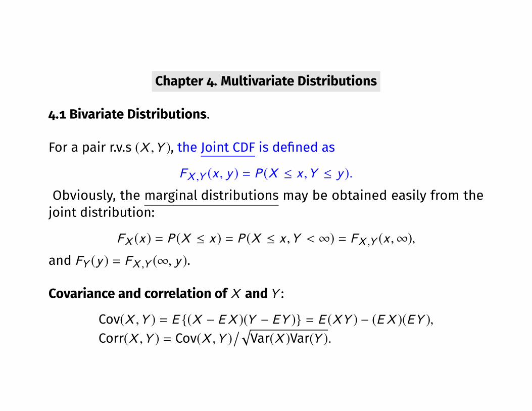
Chapter 4. Multivariate Distributions

4.1 Bivariate Distributions.

For a pair r.v.s (X ,Y ), the Joint CDF is de�ned as

FX ,Y (x , y ) = P (X ≤ x ,Y ≤ y ).

Obviously, the marginal distributions may be obtained easily from thejoint distribution:

FX (x ) = P (X ≤ x ) = P (X ≤ x ,Y < ∞) = FX ,Y (x ,∞),

and FY (y ) = FX ,Y (∞, y ).

Covariance and correlation of X andY :

Cov(X ,Y ) = E {(X − EX )(Y − EY )} = E (XY ) − (EX )(EY ),Corr(X ,Y ) = Cov(X ,Y )

/√Var(X )Var(Y ).

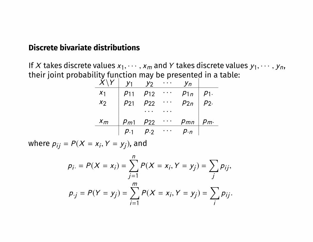
Discrete bivariate distributions

If X takes discrete values x1, · · · , xm andY takes discrete values y1, · · · , yn ,their joint probability function may be presented in a table:

X \Y y1 y2 · · · ynx1 p11 p12 · · · p1n p1·x2 p21 p22 · · · p2n p2·

· · · · · ·

xm pm1 p22 · · · pmn pm ·p ·1 p ·2 · · · p ·n

where pi j = P (X = xi ,Y = yj ), and

pi · = P (X = xi ) =n∑j=1

P (X = xi ,Y = yj ) =∑j

pi j ,

p ·j = P (Y = yj ) =m∑i=1

P (X = xi ,Y = yj ) =∑i

pi j .

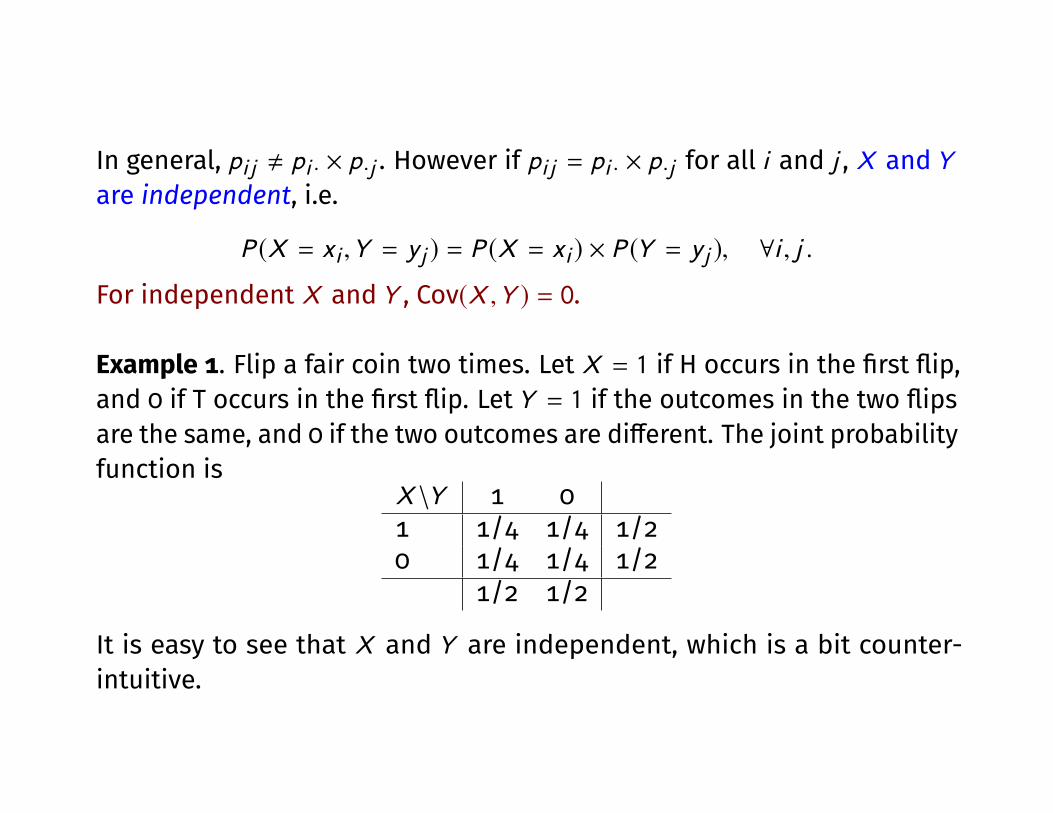
In general, pi j , pi · × p ·j . However if pi j = pi · × p ·j for all i and j , X andYare independent, i.e.

P (X = xi ,Y = yj ) = P (X = xi ) × P (Y = yj ), [i , j .

For independent X andY , Cov(X ,Y ) = 0.

Example 1. Flip a fair coin two times. Let X = 1 if H occurs in the �rst �ip,and 0 if T occurs in the �rst �ip. LetY = 1 if the outcomes in the two �ipsare the same, and 0 if the two outcomes are di�erent. The joint probabilityfunction is

X \Y 1 01 1/4 1/4 1/20 1/4 1/4 1/2

1/2 1/2

It is easy to see that X and Y are independent, which is a bit counter-intuitive.

Continuous bivariate distribution

If the CDF FX ,Y can be written as

FX ,Y (x , y ) =

∫ y

−∞

∫ x

−∞fX ,Y (u,v )dudv for any x and y ,

where fX ,Y ≥ 0, (X ,Y ) has a continuous joint distribution, and fX ,Y (x , y )is the joint PDF.

As FX ,Y (∞,∞) = 1, it holds that∫ ∞−∞

∫ ∞−∞

fX ,Y (u,v )dudv = 1.

In fact„ any non-negative function satisfying this condition is a PDF.Furthermore for any subset A in R2,

P {(X ,Y ) ∈ A} =

∫AfX ,Y (x , y )dxdy .

Also

Cov(X ,Y ) =∫(x − EX )(y − EY )fX ,Y (x , y )dxdy

=

∫x yfX ,Y (x , y )dxdy − EX EY .

Note that

FX (x ) = FX ,Y (x ,∞) =

∫ ∞−∞

∫ x

−∞fX ,Y (u,v )dudv =

∫ x

−∞

{ ∫ ∞−∞

fX ,Y (u,v )dv}du,

hence the marginal PDF of X can be derived from the joint PDF as follows

fX (x ) =

∫ ∞−∞

fX ,Y (x , y )dy .

Similarly, fy (y ) =∫ ∞−∞

fX ,Y (x , y )dx .

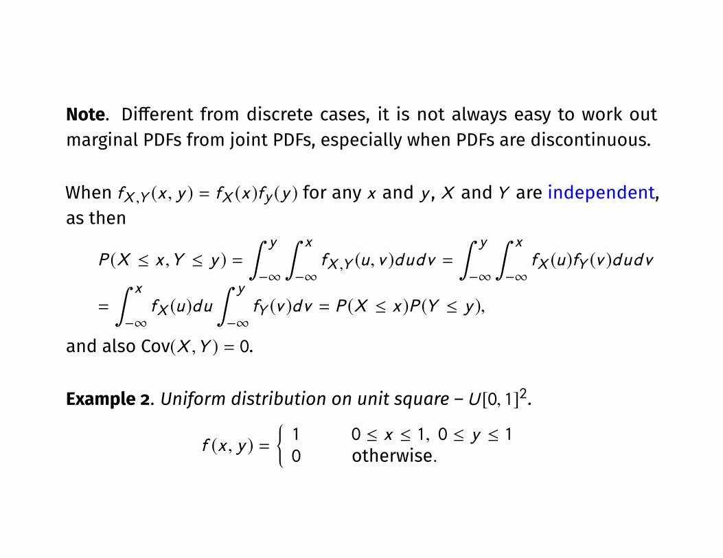
Note. Di�erent from discrete cases, it is not always easy to work outmarginal PDFs from joint PDFs, especially when PDFs are discontinuous.

When fX ,Y (x , y ) = fX (x )fy (y ) for any x and y , X andY are independent,as then

P (X ≤ x ,Y ≤ y ) =

∫ y

−∞

∫ x

−∞fX ,Y (u,v )dudv =

∫ y

−∞

∫ x

−∞fX (u)fY (v )dudv

=

∫ x

−∞fX (u)du

∫ y

−∞fY (v )dv = P (X ≤ x )P (Y ≤ y ),

and also Cov(X ,Y ) = 0.

Example 2. Uniform distribution on unit square – U [0, 1]2.

f (x , y ) =

{1 0 ≤ x ≤ 1, 0 ≤ y ≤ 10 otherwise.

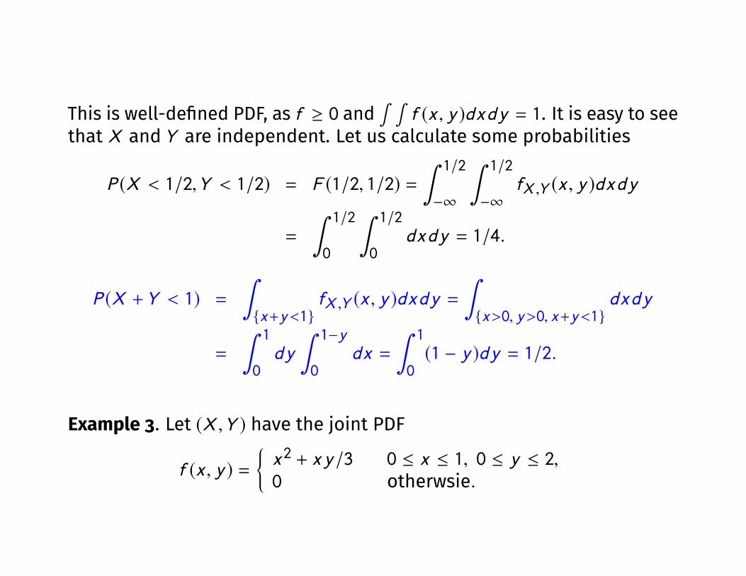
This is well-de�ned PDF, as f ≥ 0 and∫ ∫

f (x , y )dxdy = 1. It is easy to seethat X andY are independent. Let us calculate some probabilities

P (X < 1/2,Y < 1/2) = F (1/2, 1/2) =

∫ 1/2

−∞

∫ 1/2

−∞fX ,Y (x , y )dxdy

=

∫ 1/2

0

∫ 1/2

0dxdy = 1/4.

P (X +Y < 1) =

∫{x+y<1}

fX ,Y (x , y )dxdy =

∫{x>0, y>0, x+y<1}

dxdy

=

∫ 1

0dy

∫ 1−y

0dx =

∫ 1

0(1 − y )dy = 1/2.

Example 3. Let (X ,Y ) have the joint PDF

f (x , y ) =

{x2 + x y/3 0 ≤ x ≤ 1, 0 ≤ y ≤ 2,0 otherwsie.

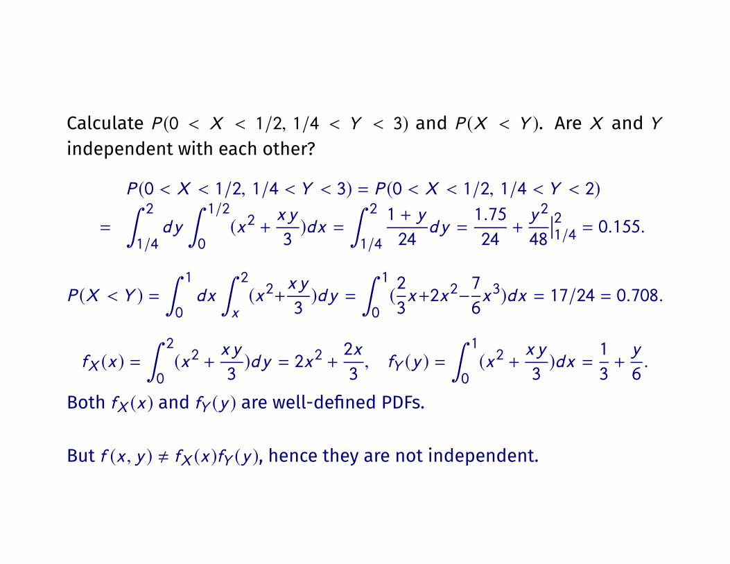
Calculate P (0 < X < 1/2, 1/4 < Y < 3) and P (X < Y ). Are X and Yindependent with each other?

P (0 < X < 1/2, 1/4 < Y < 3) = P (0 < X < 1/2, 1/4 < Y < 2)

=

∫ 2

1/4dy

∫ 1/2

0(x2 +

x y

3)dx =

∫ 2

1/4

1 + y

24dy =

1.75

24+y 2

48

��21/4 = 0.155.

P (X < Y ) =

∫ 1

0dx

∫ 2

x(x2+

x y

3)dy =

∫ 1

0(2

3x+2x2−

7

6x3)dx = 17/24 = 0.708.

fX (x ) =

∫ 2

0(x2 +

x y

3)dy = 2x2 +

2x

3, fY (y ) =

∫ 1

0(x2 +

x y

3)dx =

1

3+y

6.

Both fX (x ) and fY (y ) are well-de�ned PDFs.

But f (x , y ) , fX (x )fY (y ), hence they are not independent.

4.2 Conditional Distributions

If X andY are not independent, knowing X should be helpful in deter-mining Y , as X may carry some information on Y . Therefore it makessense to de�ne the distribution ofY given, say, X = x . This is the conceptof conditional distributions.

If both X andY are discrete, the conditional probability function is simplya special case of conditional probabilities:

P (Y = y |X = x ) = P (Y = y , X = x )/P (X = x ).

However this de�nition does not extend to continuous r.v.s, as thenP (X = x ) = 0.

De�nition (Conditional PDF). For continuous r.v.s X andY , the conditionalPDF ofY given X = x is

fY |X (·|x ) = fX ,Y (x , ·)/fX (x ).

Remark. (i) As a function of y , fY |X (y |x ) is a PDF:

P (Y ∈ A |X = x ) =

∫AfY |X (y |x )dy ,

while x is treated as a constant (i.e. not a variable).

(ii) E (Y |X = x ) =∫yfY |X (y |x )dy is a function of x , and

Var(Y |X = x ) =

∫{y − E (Y |X = x )}2fY |X (y |x )dy .

(iii) If X andY are independent, fY |X (y |x ) = fY (y ).

(iv) fX ,Y (x , y ) = fX (x )fY |X (y |x ) = fX |Y (x |y )fY (y ), which o�ers alternativeways to determine the joint PDF.

(v) E {E (Y |X )} = E (Y ) — This in fact holds for any r.v.s X andY . We give aproof here for continuous r.v.s only:

E {E (Y |X )} =

∫ { ∫yfY |X (y |x )dy

}fX (x )dx =

∫ ∫yfX ,Y (x , y )dxdy

=

∫y{ ∫

fX ,Y (x , y )dx}dy =

∫yfY (y )dy = EY .

Example 4. Let fX ,Y (x , y ) = e−y for 0 < x < y < ∞, and 0 otherwise. FindfY |X (y |x ), fX |Y (x |y ) and Cov(X ,Y ).

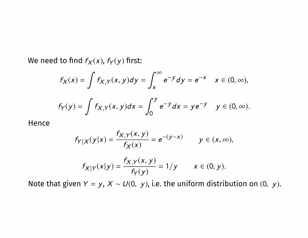
We need to �nd fX (x ), fY (y ) �rst:

fX (x ) =

∫fX ,Y (x , y )dy =

∫ ∞x

e−ydy = e−x x ∈ (0,∞),

fY (y ) =

∫fX ,Y (x , y )dx =

∫ y

0e−ydx = ye−y y ∈ (0,∞).

Hence

fY |X (y |x ) =fX ,Y (x , y )

fX (x )= e−(y−x ) y ∈ (x ,∞),

fX |Y (x |y ) =fX ,Y (x , y )

fY (y )= 1/y x ∈ (0, y ).

Note that givenY = y , X ∼ U (0, y ), i.e. the uniform distribution on (0, y ).

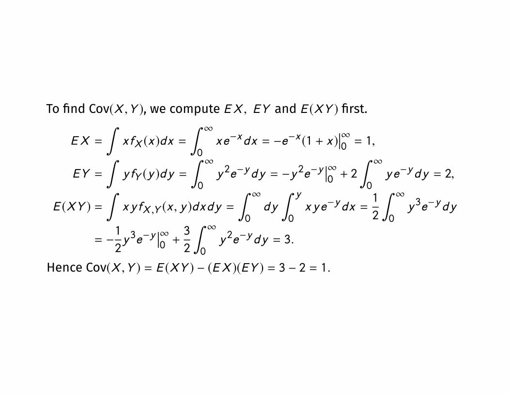
To �nd Cov(X ,Y ), we compute EX , EY and E (XY ) �rst.

EX =

∫xfX (x )dx =

∫ ∞0

xe−xdx = −e−x (1 + x )��∞0 = 1,

EY =

∫yfY (y )dy =

∫ ∞0

y 2e−ydy = −y 2e−y��∞0 + 2

∫ ∞0

ye−ydy = 2,

E (XY ) =

∫x yfX ,Y (x , y )dxdy =

∫ ∞0

dy

∫ y

0x ye−ydx =

1

2

∫ ∞0

y 3e−ydy

= −1

2y 3e−y

��∞0 +

3

2

∫ ∞0

y 2e−ydy = 3.

Hence Cov(X ,Y ) = E (XY ) − (EX )(EY ) = 3 − 2 = 1.

4.3 Multivariate Distributions

Let X = (X1, · · · ,Xn)′ be a random vector (r.v.) consisting of n r.v.s. The

joint CDF is de�ned as

F (x1, · · · , xn) ≡ FX1,··· ,Xn (x1, · · · , xn) = P (X1 ≤ x1, · · · , Xn ≤ xn).

If X is continuous, its PDF f satis�es

F (x1, · · · , xn) =

∫ xn

−∞· · ·

∫ x1

−∞f (u1, · · · ,un)du1 · · · dun .

In general, the PDF admits the factorisation

f (x1, · · · , xn) = f (x1)f (x2 |x1)f (x3 |x1, x2) · · · f (xn |x1, · · · , xn−1),

where f (xj |x1, · · · , xj−1) denotes the conditional PDF of Xj given X1 =

x1, · · · ,Xj−1 = xj .

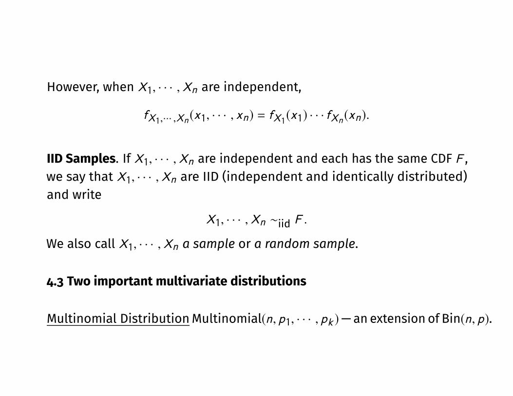
However, when X1, · · · ,Xn are independent,

fX1,··· ,Xn (x1, · · · , xn) = fX1(x1) · · · fXn (xn).

IID Samples. If X1, · · · ,Xn are independent and each has the same CDF F ,we say that X1, · · · ,Xn are IID (independent and identically distributed)and write

X1, · · · ,Xn ∼iid F .

We also call X1, · · · ,Xn a sample or a random sample.

4.3 Two important multivariate distributions

Multinomial DistributionMultinomial(n, p1, · · · , pk )—an extension of Bin(n, p).

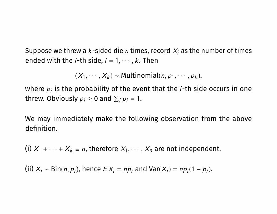
Suppose we threw a k -sided die n times, record Xi as the number of timesended with the i -th side, i = 1, · · · , k . Then

(X1, · · · ,Xk ) ∼ Multinomial(n, p1, · · · , pk ),

where pi is the probability of the event that the i -th side occurs in onethrew. Obviously pi ≥ 0 and

∑i pi = 1.

We may immediately make the following observation from the abovede�nition.

(i) X1 + · · · + Xk ≡ n , therefore X1, · · · ,Xn are not independent.

(ii) Xi ∼ Bin(n, pi ), hence EXi = npi and Var(Xi ) = npi (1 − pi ).

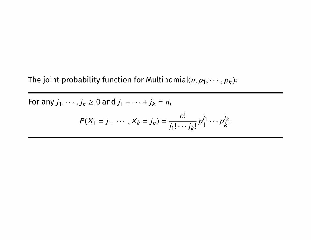
The joint probability function for Multinomial(n, p1, · · · , pk ):

For any j1, · · · , jk ≥ 0 and j1 + · · · + jk = n ,

P (X1 = j1, · · · ,Xk = jk ) =n !

j1! · · · jk !pj11· · · p

jkk.

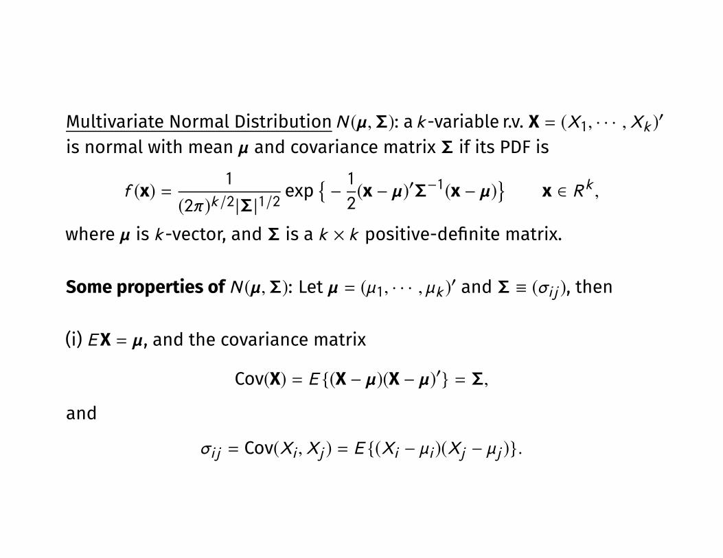
Multivariate Normal DistributionN (µ, Σ): a k -variable r.v. X = (X1, · · · ,Xk )′

is normal with mean µ and covariance matrix Σ if its PDF is

f (x) = 1

(2π)k /2 |Σ |1/2exp

{−1

2(x − µ)′Σ−1(x − µ)

}x ∈ R k ,

where µ is k -vector, and Σ is a k × k positive-de�nite matrix.

Some properties of N (µ, Σ): Let µ = (µ1, · · · , µk )′ and Σ ≡ (σi j ), then

(i) EX = µ, and the covariance matrix

Cov(X) = E {(X − µ)(X − µ)′} = Σ,

and

σi j = Cov(Xi ,Xj ) = E {(Xi − µi )(Xj − µj )}.

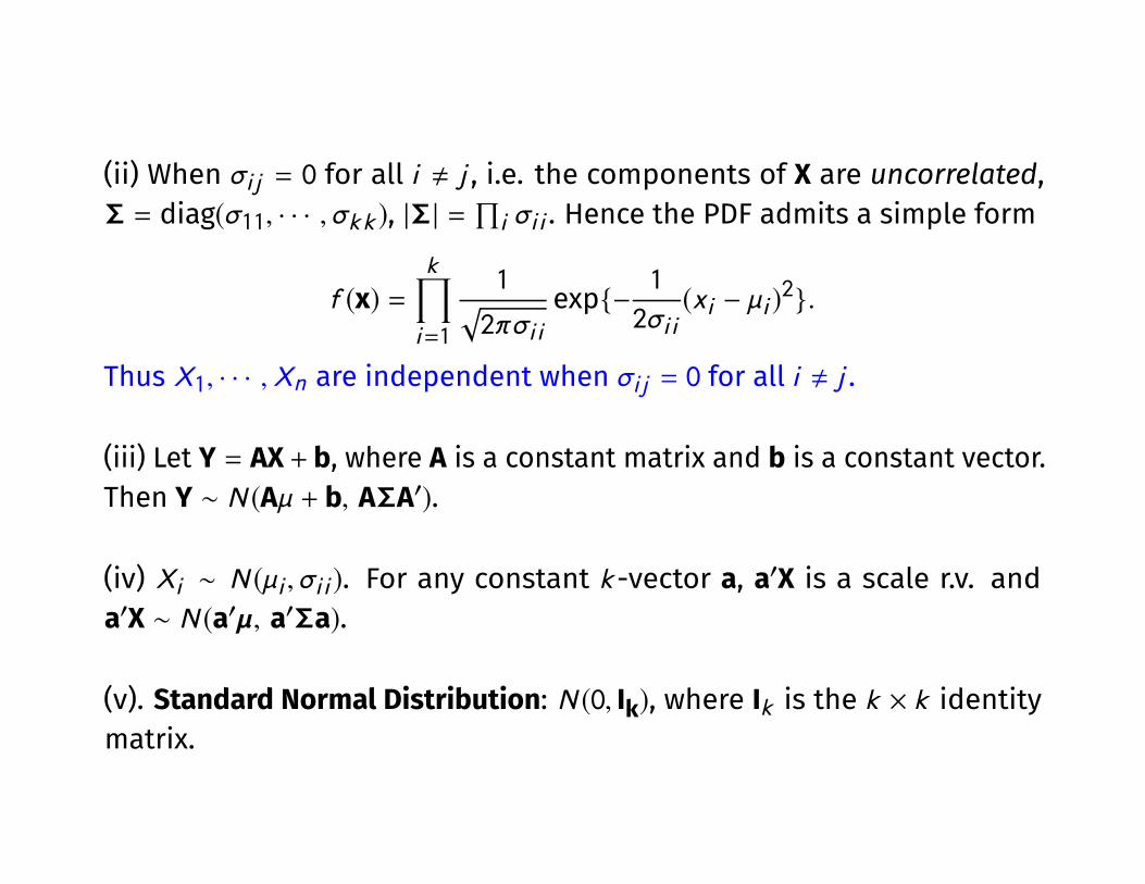
(ii) When σi j = 0 for all i , j , i.e. the components of X are uncorrelated,Σ = diag(σ11, · · · ,σk k ), |Σ | =

∏i σi i . Hence the PDF admits a simple form

f (x) =k∏i=1

1√2πσi i

exp{− 1

2σi i(xi − µi )

2}.

Thus X1, · · · ,Xn are independent when σi j = 0 for all i , j .

(iii) Let Y = AX + b, where A is a constant matrix and b is a constant vector.Then Y ∼ N (Aµ + b, AΣA′).

(iv) Xi ∼ N (µi ,σi i ). For any constant k -vector a, a′X is a scale r.v. anda′X ∼ N (a′µ, a′Σa).

(v). Standard Normal Distribution: N (0, Ik), where Ik is the k × k identitymatrix.

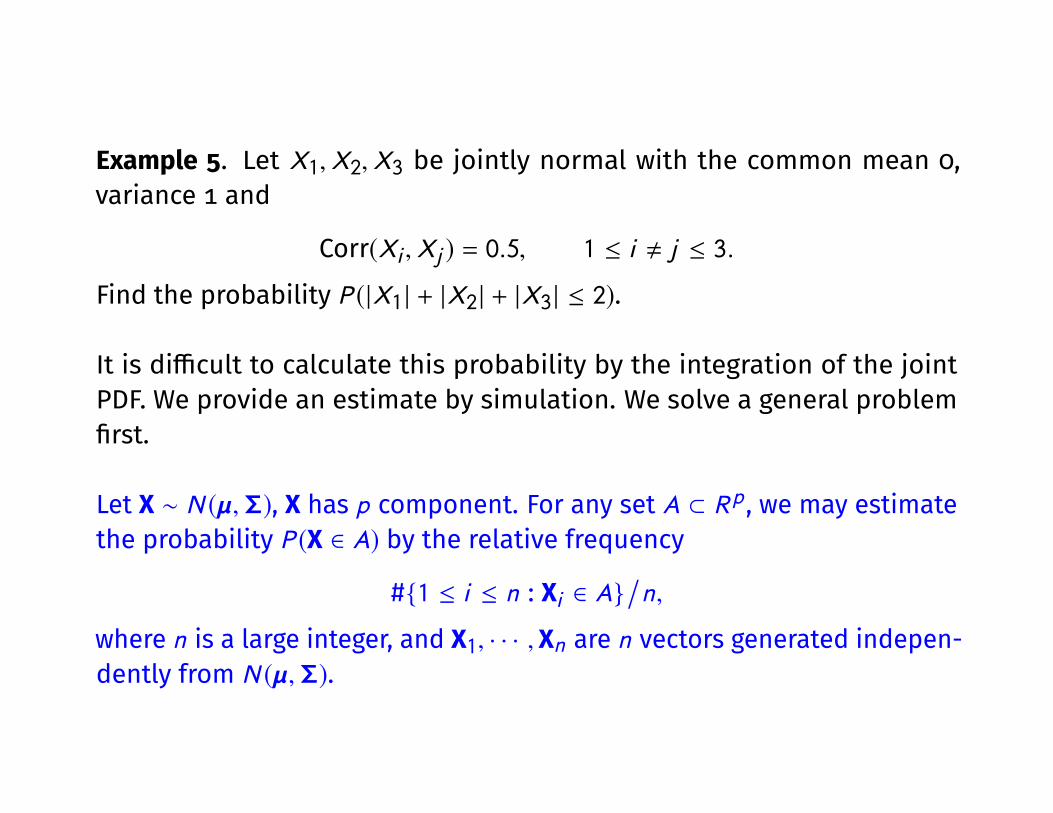
Example 5. Let X1,X2,X3 be jointly normal with the common mean 0,variance 1 and

Corr(Xi ,Xj ) = 0.5, 1 ≤ i , j ≤ 3.

Find the probability P (|X1 | + |X2 | + |X3 | ≤ 2).

It is di�cult to calculate this probability by the integration of the jointPDF. We provide an estimate by simulation. We solve a general problem�rst.

Let X ∼ N (µ, Σ), X has p component. For any set A ⊂ Rp , we may estimatethe probability P (X ∈ A) by the relative frequency

#{1 ≤ i ≤ n : Xi ∈ A}/n,

where n is a large integer, and X1, · · · , Xn are n vectors generated indepen-dently from N (µ, Σ).

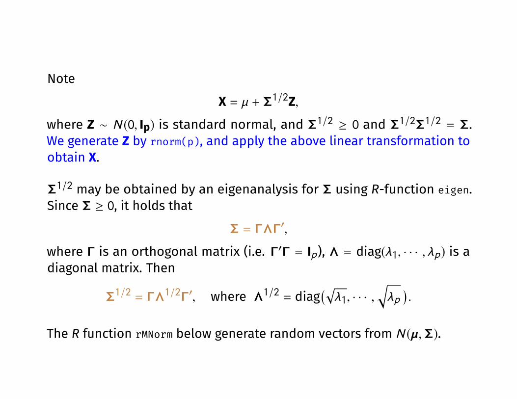
Note

X = µ + Σ1/2Z,

where Z ∼ N (0, Ip) is standard normal, and Σ1/2 ≥ 0 and Σ1/2Σ1/2 = Σ.We generate Z by rnorm(p), and apply the above linear transformation toobtain X.

Σ1/2 may be obtained by an eigenanalysis for Σ using R-function eigen.Since Σ ≥ 0, it holds that

Σ = ΓΛΓ′,

where Γ is an orthogonal matrix (i.e. Γ′Γ = Ip), Λ = diag(λ1, · · · , λp) is adiagonal matrix. Then

Σ1/2 = ΓΛ1/2Γ′, where Λ1/2 = diag(√λ1, · · · ,

√λp

).

The R function rMNorm below generate random vectors from N (µ, Σ).

rMNorm <- function(n, p, mu, Sigma) {# generate n p-vectors from N(mu, Sigma)# mu is p-vector of mean, Sigma >=0 is pxp matrix

t <- eigen(Sigma, symmetric=T) # eigenanalysis for Sigmaev <- sqrt(t$values) # square-roots of the eigenvaluesG <- as.matrix(t$vectors) # line up eigenvectors into a matrix GD <- G*0; for(i in 1:p) D[i,i] <- ev[i]; # D is diagonal matrixP <- G%*%D%*%t(G) # P=GDG' is the required transformation matrixZ <- matrix(rnorm(n*p), byrow=T, ncol=p)# Z is nxp matrix with elements drawn from N(0,1)

Z <- Z%*%P # Now each row of Z is N(0, Sigma)X <- matrix(rep(mu, n), byrow=T, ncol=p) + Z

# each row of X is N(mu, Sigma)}

This function is saved in the �le ‘rMNorm.r’. We may use it to perform therequired task:

source("rMNorm.r")

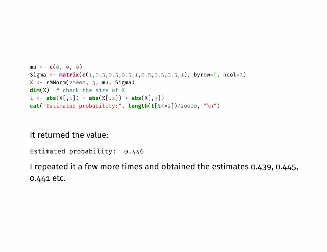
mu <- c(0, 0, 0)Sigma <- matrix(c(1,0.5,0.5,0.5,1,0.5,0.5,0.5,1), byrow=T, ncol=3)X <- rMNorm(20000, 3, mu, Sigma)dim(X) # check the size of Xt <- abs(X[,1]) + abs(X[,2]) + abs(X[,3])cat("Estimated probability:", length(t[t<=2])/20000, "\n")

It returned the value:

Estimated probability: 0.446

I repeated it a few more times and obtained the estimates 0.439, 0.445,0.441 etc.

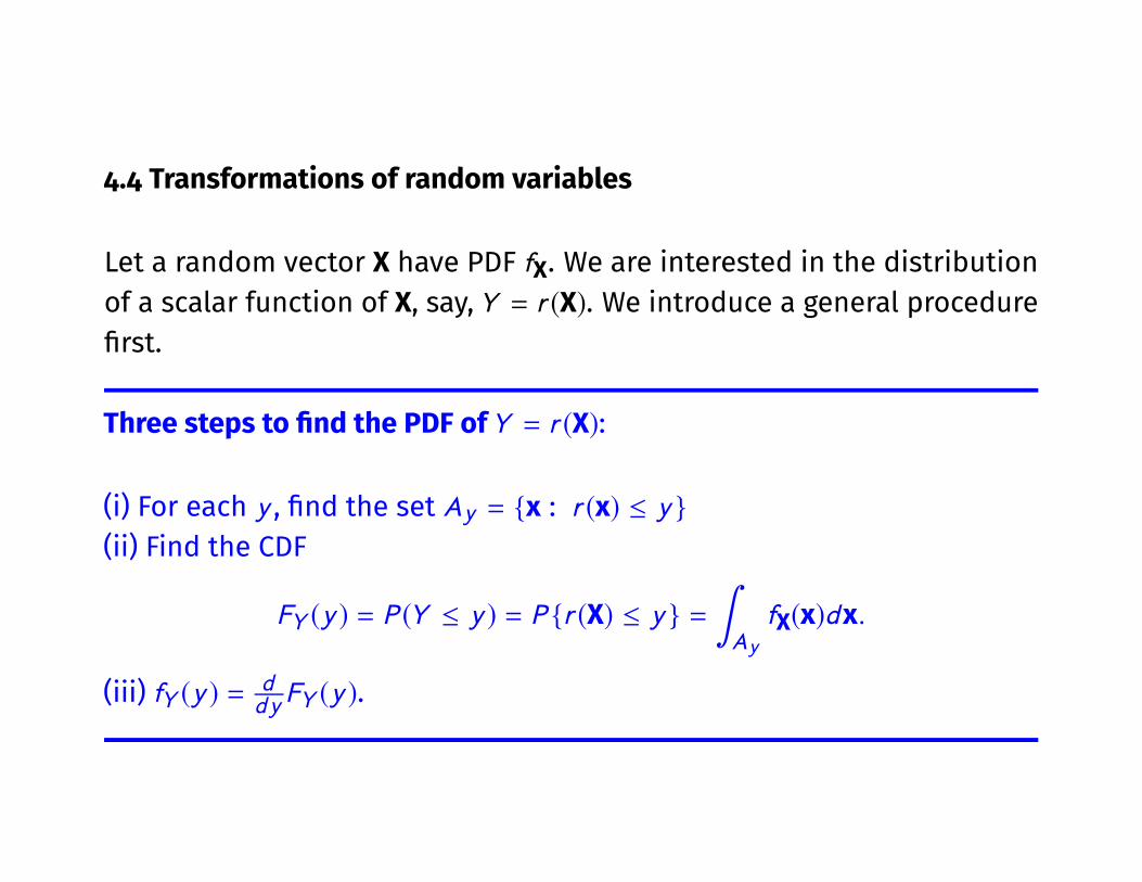
4.4 Transformations of random variables

Let a random vector X have PDF fX. We are interested in the distributionof a scalar function of X, say,Y = r (X). We introduce a general procedure�rst.

Three steps to �nd the PDF ofY = r (X):

(i) For each y , �nd the set Ay = {x : r (x) ≤ y }(ii) Find the CDF

FY (y ) = P (Y ≤ y ) = P {r (X) ≤ y } =∫AyfX(x)dx.

(iii) fY (y ) = ddy FY (y ).

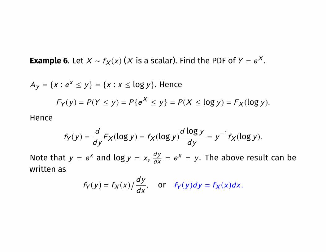
Example 6. Let X ∼ fX (x ) (X is a scalar). Find the PDF ofY = eX .

Ay = {x : ex ≤ y } = {x : x ≤ log y }. Hence

FY (y ) = P (Y ≤ y ) = P {eX ≤ y } = P (X ≤ log y ) = FX (log y ).

Hence

fY (y ) =d

dyFX (log y ) = fX (log y )

d log ydy

= y−1fX (log y ).

Note that y = ex and log y = x , dydx = ex = y . The above result can bewritten as

fY (y ) = fX (x )/dydx, or fY (y )dy = fX (x )dx .

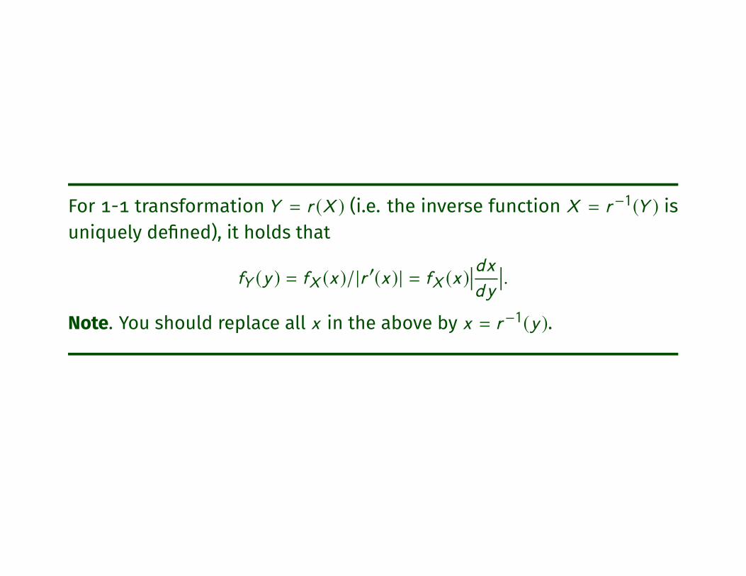
For 1-1 transformationY = r (X ) (i.e. the inverse function X = r−1(Y ) isuniquely de�ned), it holds that

fY (y ) = fX (x )/|r′(x )| = fX (x )

��dxdy

��.Note. You should replace all x in the above by x = r−1(y ).

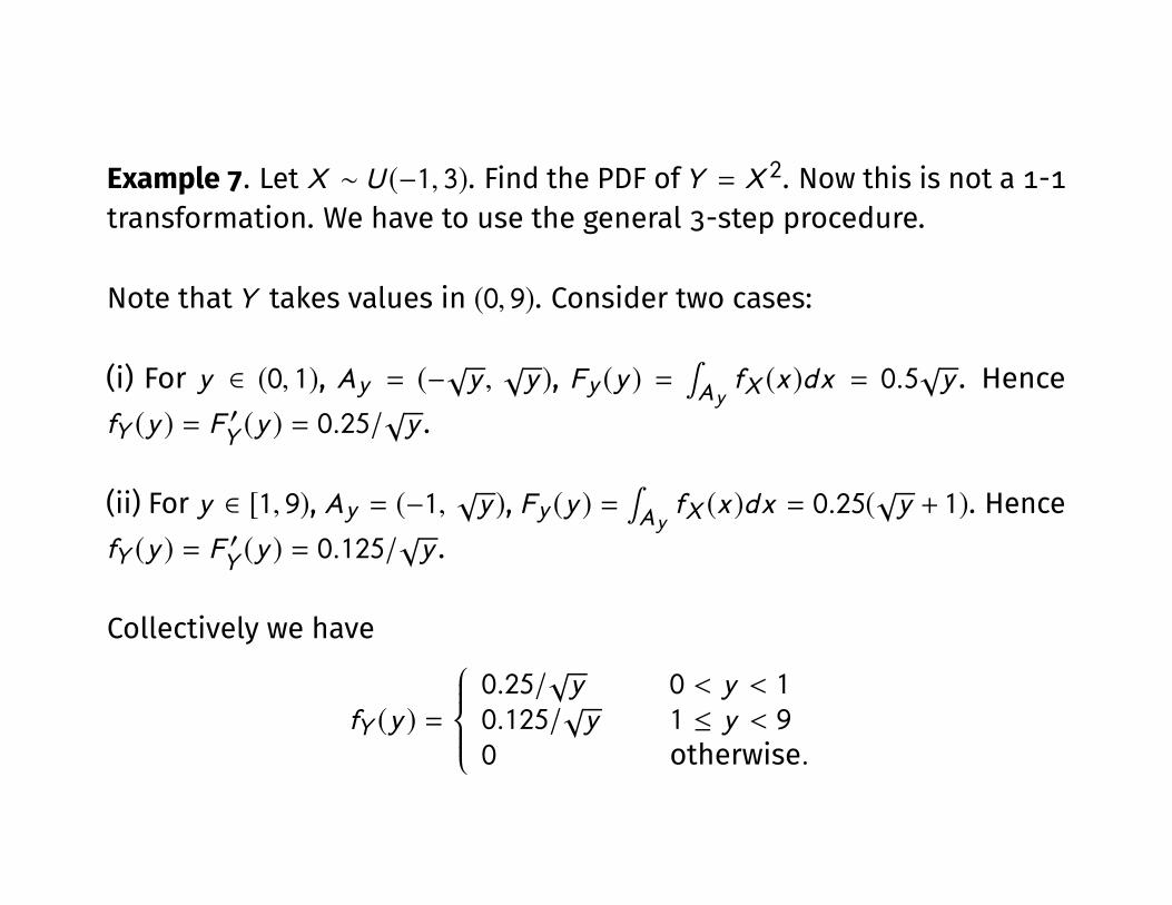
Example 7. Let X ∼ U (−1, 3). Find the PDF ofY = X 2. Now this is not a 1-1transformation. We have to use the general 3-step procedure.

Note thatY takes values in (0, 9). Consider two cases:

(i) For y ∈ (0, 1), Ay = (−√y ,√y ), Fy (y ) =

∫AyfX (x )dx = 0.5

√y . Hence

fY (y ) = F′Y(y ) = 0.25/

√y .

(ii) For y ∈ [1, 9), Ay = (−1,√y ), Fy (y ) =

∫AyfX (x )dx = 0.25(

√y + 1). Hence

fY (y ) = F′Y(y ) = 0.125/

√y .

Collectively we have

fY (y ) =

0.25/

√y 0 < y < 1

0.125/√y 1 ≤ y < 9

0 otherwise.