99

CHAPTER 4

LOCATION OF FAULTS IN TRANSFORMERS

DURING IMPULSE TESTING

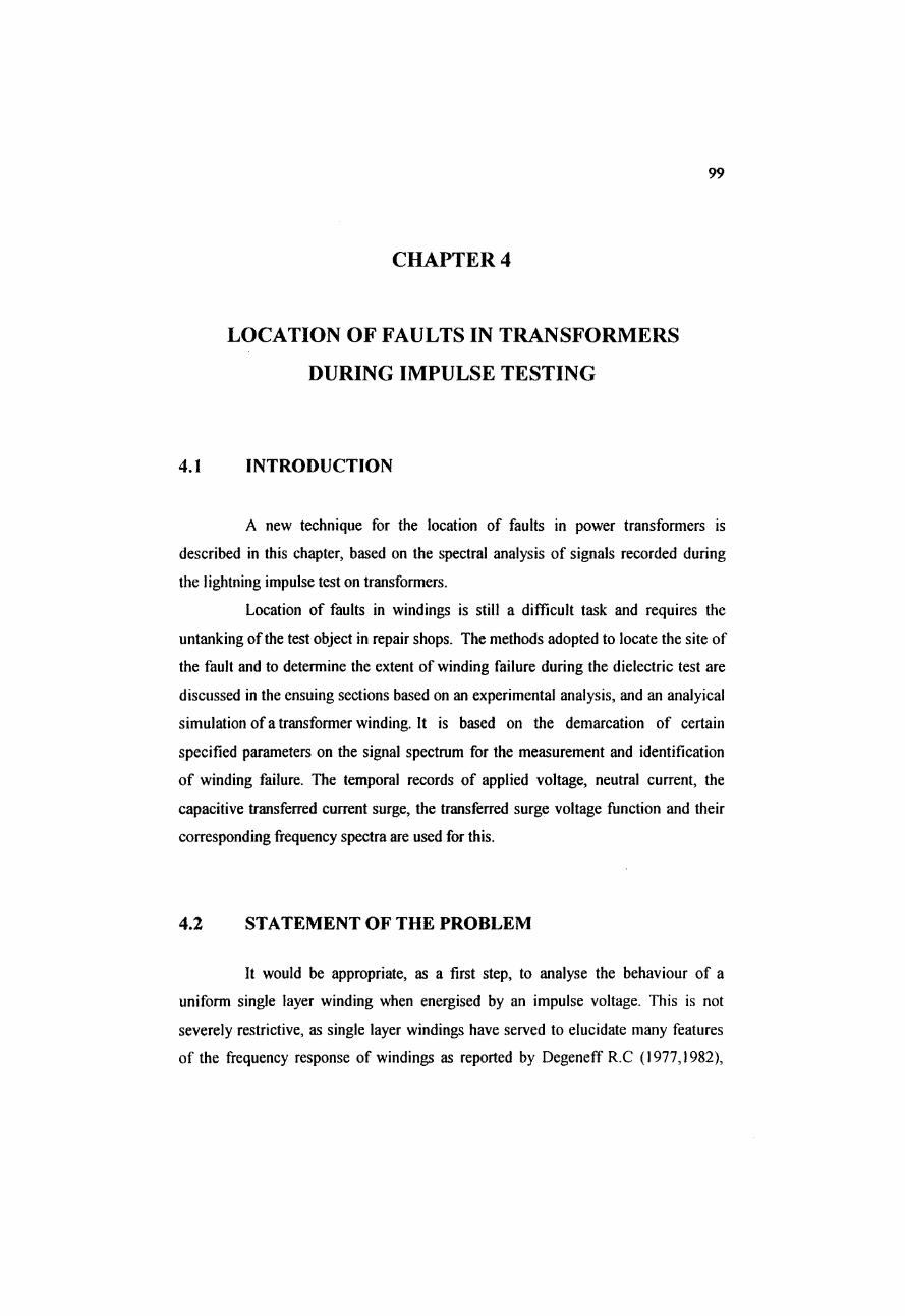
4.1 INTRODUCTION

A new technique for the location of faults in power transformers is

described in this chapter, based on the spectral analysis of signals recorded during

the lightning impulse test on transformers.

Location of faults in windings is still a difficult task and requires the

untanking of the test object in repair shops. The methods adopted to locate the site of

the fault and to determine the extent of winding failure during the dielectric test are

discussed in the ensuing sections based on an experimental analysis, and an analyical

simulation of a transformer winding. It is based on the demarcation of certain

specified parameters on the signal spectrum for the measurement and identification

of winding failure. The temporal records of applied voltage, neutral current, the

capacitive transferred current surge, the transferred surge voltage function and their

corresponding frequency spectra are used for this.

4.2 STATEMENT OF THE PROBLEM

It would be appropriate, as a first step, to analyse the behaviour of a

uniform single layer winding when energised by an impulse voltage. This is not

severely restrictive, as single layer windings have served to elucidate many features

of the frequency response of windings as reported by Degeneff R.C (1977,1982),

100

Dick E.P and Erven C.C (1978). Further, with adequate mathematical underpinning,

results from such a winding can form the basis for a more generalised treatment for

power transformer applications.

The aims of this chapter are as follows:

1) To propose methods for location of winding fault during impulse

tests.

2) To assess the magnitude of failure of winding.

3) To confirm the utility of the methods with experimental results.

In all cases, the term fault, here refers to a breakdown across a section of

the winding during the impulse test. The following sections discuss the case of a

breakdown of non-restoring insulation. This is not a trivial issue as several

investigations use differing principles for analysing faults during impulse tests. For

example, Malewski R and Poulin B (1985) state that the appearance of fault on the

neutral current is similar to that observed when a portion of the winding is physically

short by a piece of wire.

Malewski R. and Poulin B (1988) used a diac across sections for

elucidating certain features with the transfer function method for discharge analysis.

This chapter progresses with the above conceptual approach to simulate fault

phenomenon in windings.

4.3 SIMULATION OF FAULT

Analysis is done on records obtained from experimental and analytical

simulation during impulse testing. An exercise is done for this by deliberately

connecting a fault simulating model across the section to be faulted which creates a

destructive fault within windings. The applied voltage, and the winding current

101

response prior to and after placing the short are recorded and their difference is

evaluated for failure analysis as explained in chapter 2.

4.3.1 EXPERIMENTAL ANALYSIS

The experimental verification is done on a specially constructed layer

winding transformer model having the high voltage coil built with 20 tapping

arrangement over the length and housed with a grounded metal core and shield as

described in Appendix 1. It differs from the Abetti coil in this respect that it has a

secondary winding, which could be used for additional measurement and also has a

low value ground capacitance Cg due to the presence of additional metallic former in

the inner and outer diameter.

The fault model for the experimental analysis of inter-section fault uses a

neon bulb to directly short between sections of the layer winding.

The impulse test is done using a Marx generator PU12 Haefley model for

conducting an impulse or the chopped impulse test. The arrangement uses a voltage

divider, current shunt, measuring cables, the 10-bit digital storage oscilloscope and

the 12-bit HP-VXI based virtual instrument configured for the impulse testing as

described in Appendix 3. The voltage signals and current signals are recorded while

applying full or reduced level lightning impulse signal and tail chopped impulse

signals as specified in IEC 76 (1980) standards.

The experimental simulation is done by connecting the fault model

deliberately between 5% or 10% tapping of the high voltage winding as shown in

Fig. 4.1.

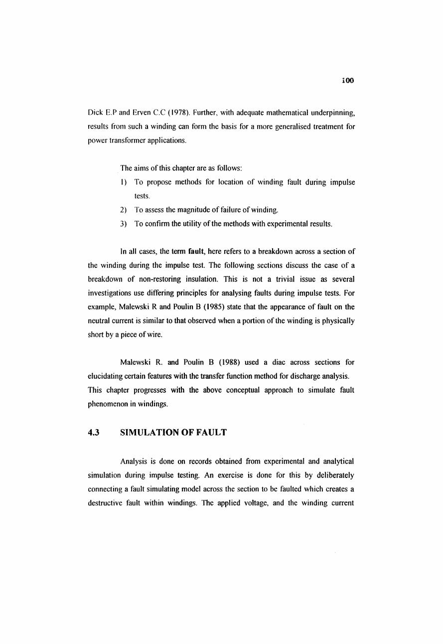
The actual observation of current records measured using current shunt,

shielded cables are as shown in Fig. 4.2.

102

-Q: CRO

Tnmfemd sazge voltage

Figure 4.1 Lightning impulse test terminal connections and methods of failure detection

43.2 DETAILS OF ANALYTICAL SIMULATION

A single layer winding often adopted in literature as a 10-section Abetti

coil and reported by Abetti P.A and Maginniss (1954), DegenefF R.C (1977),and

Jayashankar V (1994) is used as the circuit model for analytical simulation, the

details of which are given in Appendix 2. The RLC lumped parameter model has the

first few resonant frequencies as 7.39K, 16.5K, 28K, 41K.etc.

103

The relative shifts in these frequencies are used for analysis. Analytical

simulation of fault across sections of the coil is done using a time-operated switch.

The fault is created with a switch Si being connected across the section that is to be

faulted. The switch remains open for a time upto tj after the energisation of the coil

by the Marx generator. At tj the switch closes and continues to stay in the closed

position until the end of the simulation. This approach is adopted because in actual

situations, the breakdown will always occur after a finite instance if the coil has

originally not been subjected to catastrophic dielectric failure. This justifies the use

of ft.

The necessity of keeping the switch closed until breakdown is obvious

since this work mainly caters to the breakdown of non- restoring insulation.

The study uses PSPICE (Programmable Simulation Package for in Circuit

Emulation, Version 7.0) for analytical simulation.

During simulation the input voltage is obtained from a Marx generator

circuit model as a constant source. Hence, further analysis of the minor faults is done

on the current spectrum only. This is equivalent to using the transfer function (TF)

analysis.

In all impulse measurements the difference between currents at reduced

and full voltages are of primary importance. The sequence of simulations is as

follows:

1. The simulation is done for a standard lightning impulse (LI) signal initially

with no fault across the winding. The records of the applied voltage V and

winding current i are stored in files.

2. A fault is created with an initial value of tj (of 20 ps) on a portion of the

winding between 90 - 100% of its length. The records of voltage V and

winding current i are stored.

104

3. The simulation is repeated at various locations of the winding length as

top, middle, and bottom sections. Sectional short-circuit is created for 5%,

10%, 15% etc, of the percentile length of coil to simulate sectional

winding fault. The short-circuiting is done between 20%-30%, 60%-70%,

70-80%... 80-90% etc..tapping, and their files are stored.

4. The analytical simulations are also repeated for other values of h such as 5

jis, 40ps to simulate effects of breakdown at different instances of time.

This approach is justified here since it is based on the fact that transformer

windings with different insulation types have different breakdown

strength. The existence of f will accentuate the difference, if any.

The simulations are also done with impulse chopped on the tail at 2ps, 6ps

as a part of type test as specified by IEC 76 (1980) for insulation integrity tests.

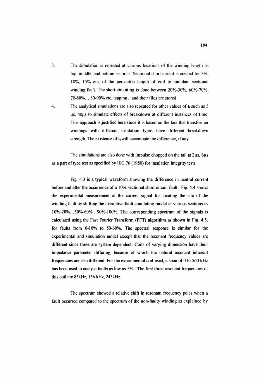
Fig. 4.3 is a typical waveform showing the difference in neutral current

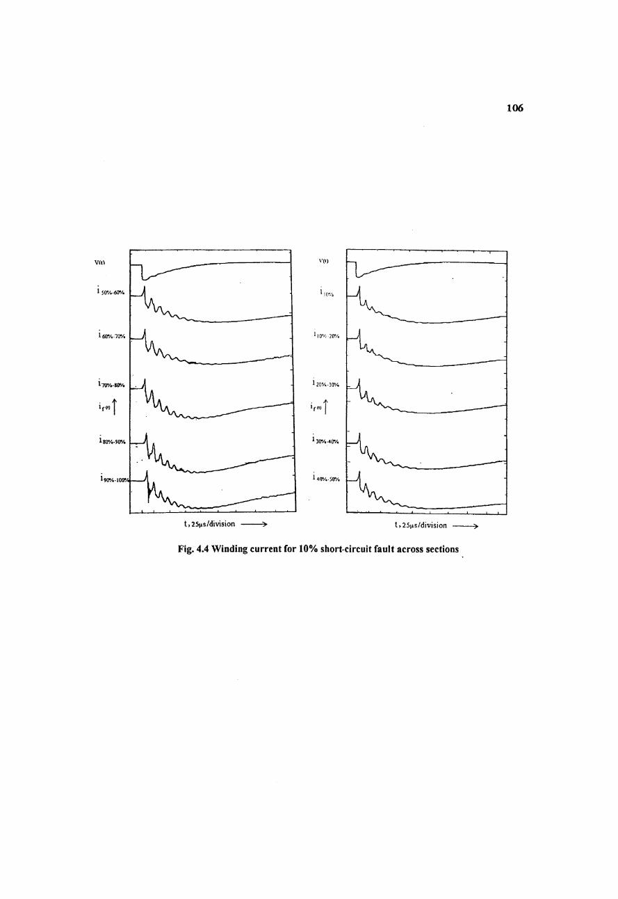
before and after the occurrence of a 10% sectional short circuit fault. Fig. 4.4 shows

the experimental measurement of the current signal for locating the site of the

winding fault by shifting the disruptive fault simulating model at various sections as

10%-20%...50%-60%...90%-100%. The corresponding spectrum of the signals is

calculated using the Fast Fourier Transform (FFT) algorithm as shown in Fig. 4.5.

for faults from 0-10% to 50-60%. The spectral response is similar for the

experimental and simulation model except that the resonant frequency values are

different since these are system dependent. Coils of varying dimension have their

impedance parameter differing, because of which the natural resonant inherent

frequencies are also different. For the experimental coil used, a span of 0 to 560 kHz

has been used to analyse faults as low as 5%. The first three resonant frequencies of

this coil are 85kHz, 156 kHz, 243kHz.

The spectrum showed a relative shift in resonant frequency poles when a

fault occurred compared to the spectrum of the non-faulty winding as explained by

Vol

tage

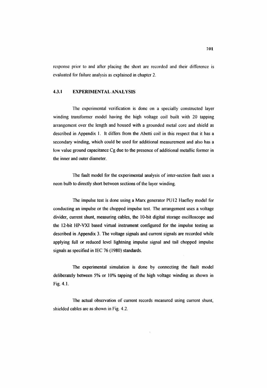
Time —> 10nsFig.4.2 Lightning impulse test records

(1) Applied Impulse voltage (2) Neutral winding current(3) Capacitive transferred current prior to fault(4) Capacitive transferred current after a fault

TeK stop: single Seq S.ooms/s

Mathl Zoom: 1657oX Vert ~ i.OX Horz

Mathl

,-j•” is ar ■Jrutrv'—m4ovoms ‘cwrHr -tteoHW1lOOmV 10.0ms

Fig. 4.3 Winding current(a) prior to fault(b) for 10% short circuit fault across a section(c) difference between record (b) and (a)

106

t,2S|js/division ------- >

Fig. 4.4 Winding current for 10% short-circuit fault across sections

107

Fig. 4.5 Spectra of winding current records from Fig. 4.4

108

Fig. 4.6 Spectra of neutral winding current (A) prior to (B) after short circuit fault

109

Degeneff R.C (1977), Malewski R and Poulin B (1988), and Jayashankar V (1994).

This is enumerated in Fig. 4.6

4.4 PROCEDURE FOR ESTIMATING FAULT LOCATION

It would appear at the first glance that time domain records would suffice

for the analysis of fault location. However, this is not possible as the instance of fault

ti can change and also in practice, the applied voltage can itself change between two

successive applications.

For this reason a frequency domain approach is used. The spectrum of the

current i(f) is obtained from the time domain record by using a standard Fast Fourier

Transform (FFT) routine.

Similarly, the spectrum of the voltage v(f)is obtained from the time

domain record of the voltage v(t).

Various parameters are obtained from the frequency spectrum, and the

variations for occurrences of fault at different locations are discussed based on the

analytical and experimental simulation.

We propose the estimation of the location of the winding fault using

specially defined variables namely, the

• Pole Variation Response (PVR)

• Amplitude Variation Response (AVR)

• Uniform Coil Resonance Parameter (UCRP)

The percentages of deviations are calculated using spectral analysis of

signals prior to and after the occurrence of fault and is given as

((Afauit — A nofault) / A nofault)* 100 (4.1)

110

where A is any of the mentioned variables. An exercise is done in the spectrum

between unfaulted and faulted conditions of the winding model using the records of

neutral winding current and transferred surge current.

The computation of the three parameters is as follows:

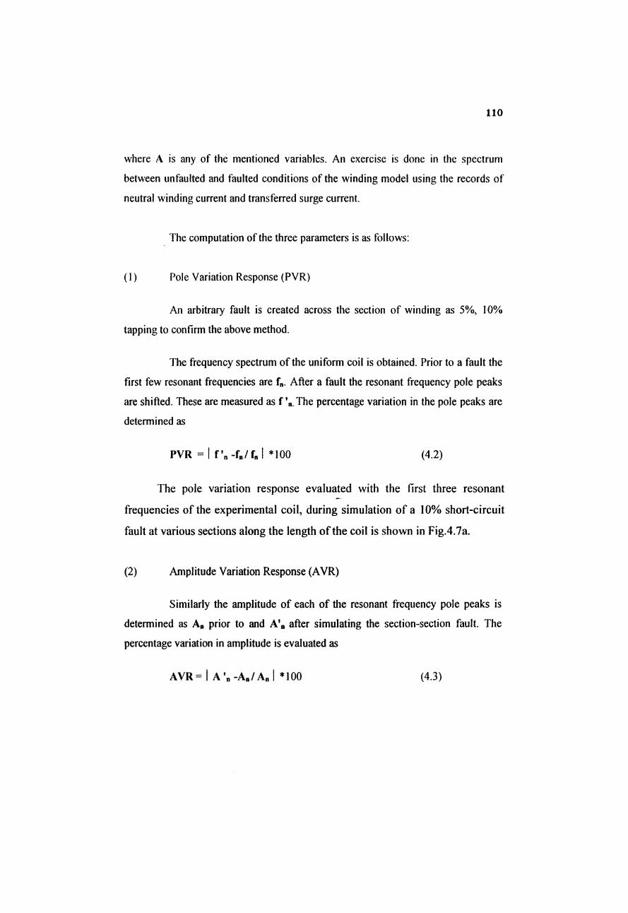
(1) Pole Variation Response (PVR)

An arbitrary fault is created across the section of winding as 5%, 10%

tapping to confirm the above method.

The frequency spectrum of the uniform coil is obtained. Prior to a fault the

first few resonant frequencies are f„. After a fault the resonant frequency pole peaks

are shifted. These are measured as f The percentage variation in the pole peaks are

determined as

PVR = I f'n-fn/fj *100 (4.2)

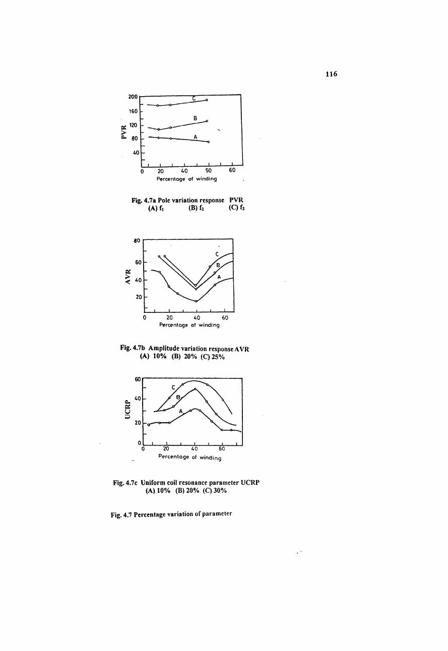
The pole variation response evaluated with the first three resonant

frequencies of the experimental coil, during simulation of a 10% short-circuit

fault at various sections along the length of the coil is shown in Fig.4.7a.

(2) Amplitude Variation Response (AVR)

Similarly the amplitude of each of the resonant frequency pole peaks is

determined as A„ prior to and A',, after simulating the section-section fault. The

percentage variation in amplitude is evaluated as

AVR= I A -A„/A„ | *100 (4.3)

Ill

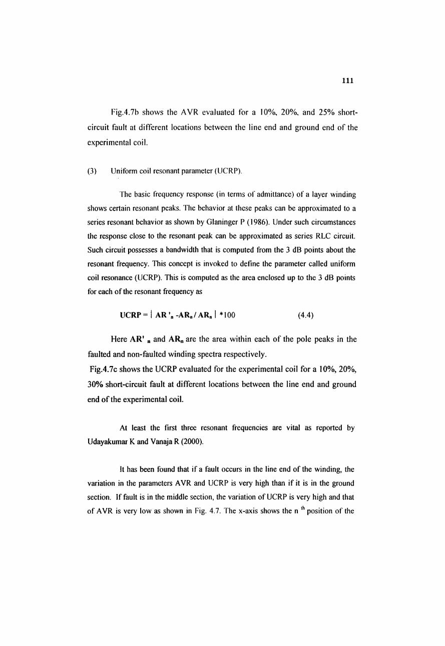
Fig.4.7b shows the AVR evaluated for a 10%, 20%, and 25% short-

circuit fault at different locations between the line end and ground end of the

experimental coil.

(3) Uniform coil resonant parameter (UCRP).

The basic frequency response (in terms of admittance) of a layer winding

shows certain resonant peaks. The behavior at these peaks can be approximated to a

series resonant behavior as shown by Glaninger P (1986). Under such circumstances

the response close to the resonant peak can be approximated as series RLC circuit.

Such circuit possesses a bandwidth that is computed from the 3 dB points about the

resonant frequency. This concept is invoked to define the parameter called uniform

coil resonance (UCRP). This is computed as the area enclosed up to the 3 dB points

for each of the resonant frequency as

UCRP = I AR -ARn / ARn I * 100 (4.4)

Here AR' „ and AR„ are the area within each of the pole peaks in the

faulted and non-faulted winding spectra respectively.

Fig.4.7c shows the UCRP evaluated for the experimental coil for a 10%, 20%,

30% short-circuit fault at different locations between the line end and ground

end of the experimental coil.

At least the first three resonant frequencies are vital as reported by

Udayakumar K and Vanaja R (2000).

It has been found that if a fault occurs in the line end of the winding, the

variation in the parameters AVR and UCRP is very high than if it is in the ground

section. If fault is in the middle section, the variation of UCRP is very high and that

of AVR is very low as shown in Fig. 4.7. The x-axis shows the n lh position of the

112

tapping of the winding from line end to ground end where n=0-10%, 10%-20%...

and the y-axis shows the respective variables evaluated using Equation (4.1).

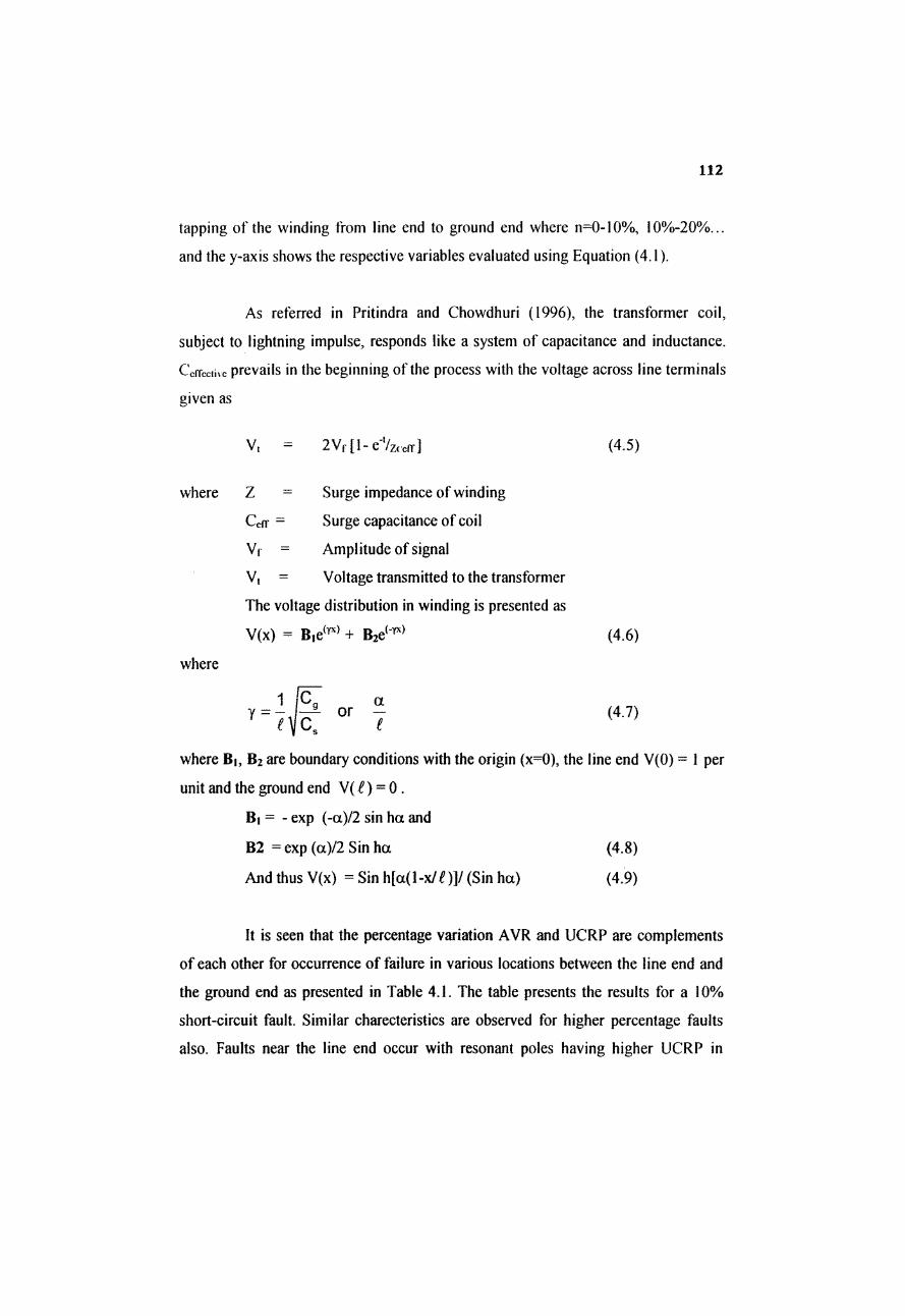
As referred in Pritindra and Chowdhuri (1996), the transformer coil,

subject to lightning impulse, responds like a system of capacitance and inductance.

Corrective prevails in the beginning of the process with the voltage across line terminals

given as

where

where

where Bj, B2 are boundary conditions with the origin (x=0), the line end V(0) = 1 per

unit and the ground end V( £) ~ 0 .

Bi = - exp (-a)/2 sin ha and

B2 = exp (a)/2 Sin ha (4.8)

And thus V(x) = Sin h[a(l-x/^)]/(Sin ha) (4.9)

It is seen that the percentage variation AVR and UCRP are complements

of each other for occurrence of failure in various locations between the line end and

the ground end as presented in Table 4.1. The table presents the results for a 10%

short-circuit fault. Similar charecteristics are observed for higher percentage faults

also. Faults near the line end occur with resonant poles having higher UCRP in

V, = 2Vr [l-e'Vzrcfr] (4.5)

Z = Surge impedance of winding

CefT = Surge capacitance of coil

Vf = Amplitude of signal

V, = Voltage transmitted to the transformer

The voltage distribution in winding is presented as

V(x) - B,e(YX) + B2e('TX) (4.6)

1 C9

Y = —I—- ornc.

a (4.7)

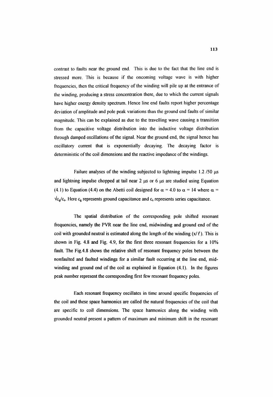
113

contrast to faults near the ground end. This is due to the fact that the line end is

stressed more. This is because if the oncoming voltage wave is with higher

frequencies, then the critical frequency of the winding will pile up at the entrance of

the winding, producing a stress concentration there, due to which the current signals

have higher energy density spectrum. Hence line end faults report higher percentage

deviation of amplitude and pole peak variations than the ground end faults of similar

magnitude. This can be explained as due to the travelling wave causing a transition

from the capacitive voltage distribution into the inductive voltage distribution

through damped oscillations of the signal. Near the ground end, the signal hence has

oscillatory current that is exponentially decaying. The decaying factor is

deterministic of the coil dimensions and the reactive impedance of the windings.

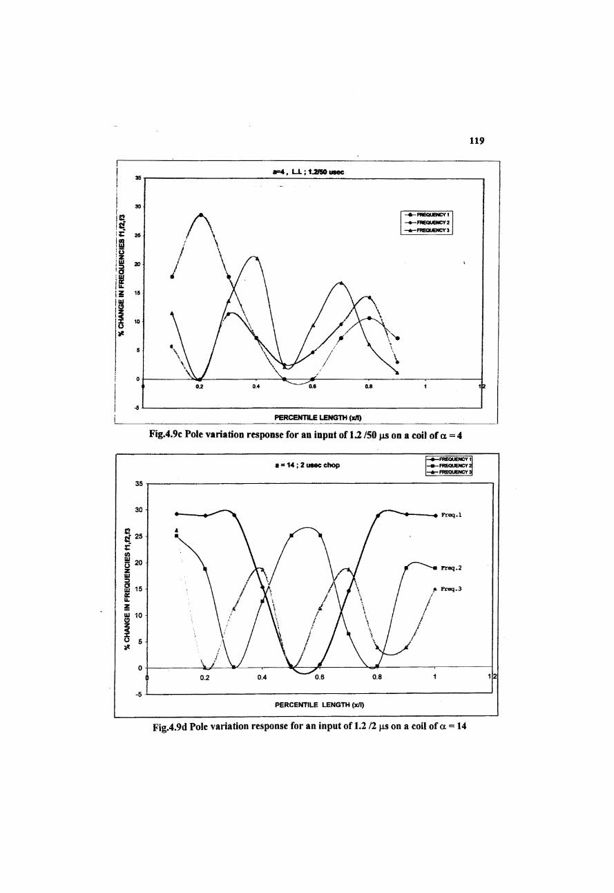
Failure analyses of the winding subjected to lightning impulse 1.2 /50 jjls

and lightning impulse chopped at tail near 2 ps or 6 ps are studied using Equation

(4.1) to Equation (4.4) on the Abetti coil designed for a = 4.0 to a = 14 where a =

Vcg/cs. Here cg represents ground capacitance and cs represents series capacitance.

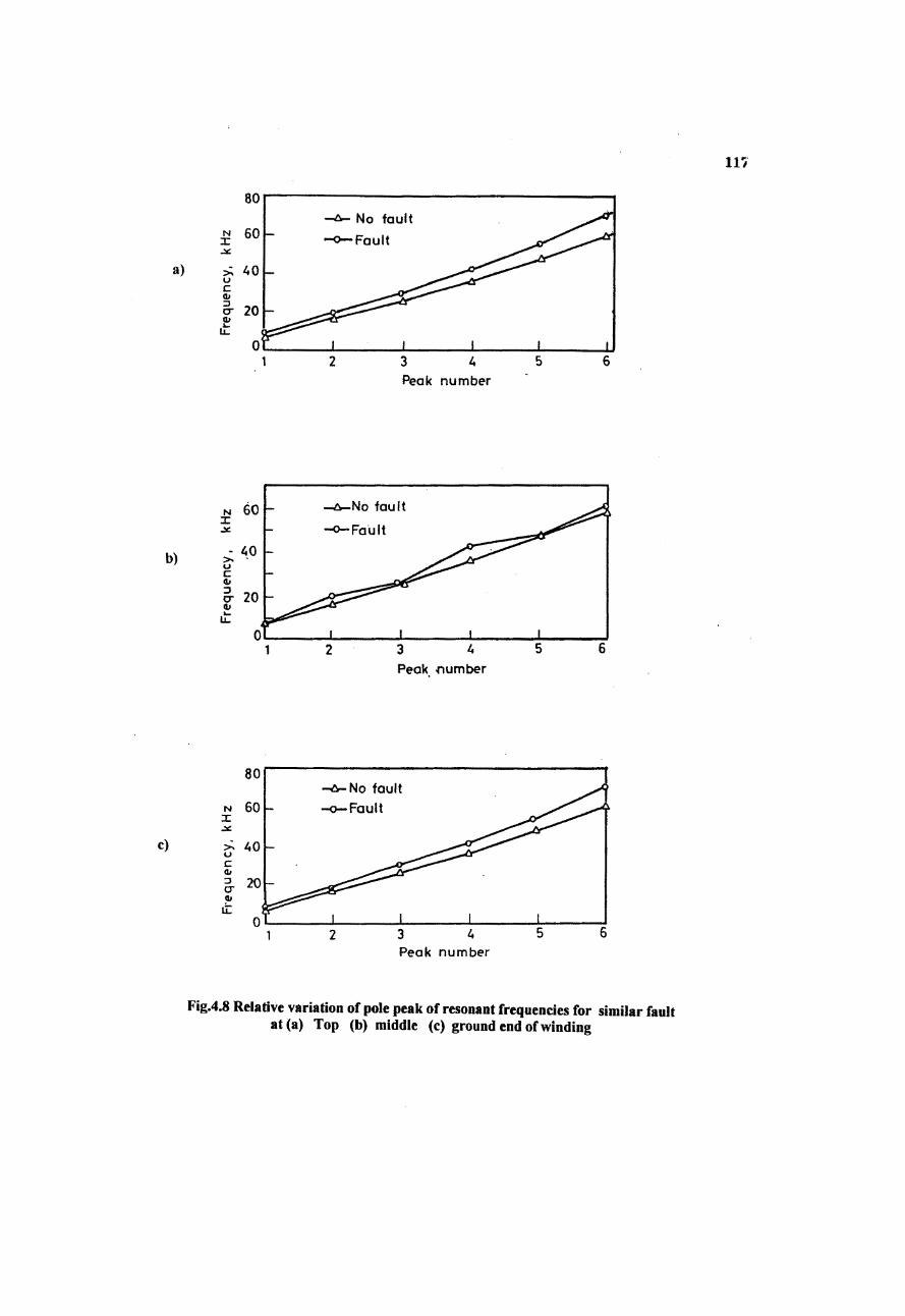
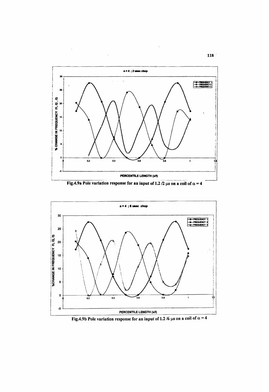
The spatial distribution of the corresponding pole shifted resonant

frequencies, namely the PVR near the line end, midwinding and ground end of the

coil with grounded neutral is estimated along the length of the winding (xH). This is

shown in Fig. 4.8 and Fig. 4.9, for the first three resonant frequencies for a 10%

fault. The Fig.4.8 shows the relative shift of resonant frequency poles between the

nonfaulted and faulted windings for a similar fault occurring at the line end, mid­

winding and ground end of the coil as explained in Equation (4.1). In the figures

peak number represent the corresponding first few resonant frequency poles.

Each resonant frequency oscillates in time around specific frequencies of

the coil and these space harmonics are called the natural frequencies of the coil that

are specific to coil dimensions. The space harmonics along the winding with

grounded neutral present a pattern of maximum and minimum shift in the resonant

114

frequency poles by evaluation using Equation (4.1) and are shown in the y-axis. The

Fig.4.9 represents clearly the relative shift for the first three space harmonics or

resonant frequency poles, with (n=3) with different a for different impulse inputs.

The first resonant frequency has a minimum deviation of the pole peak in

the mid-section of the winding than at the line end or ground end. The second

resonant frequency shows a minimum shift at the 1/4, 3/4 points and a maximum at

the V2 point of the winding, and so on for higher resonant harmonics.

From the analysis it is observed that, a fault near the line end shows a

higher variation in the fundamental frequency compared to a fault near the

midwinding and ground end. On the other hand, a fault near the midwinding shows

second resonant frequency to have a predominantly higher shift in comparison to the

odd harmonics. Similar patterns are observed for higher space harmonics also.

Table 4.1 Percentile variation in AYR and UCRP for fault

xi i Variation in % AVR Variation in % UCRP

Top 10% tapping 40-55 17-21

Middle 10% tapping 14-15 31

Bottom 10% tapping 35-45 13-14

4.5 ANALYSIS OF SIMULATION RESULTS FOR

ESTABLISHING MAGNITUDE OF FAULTS

At the first instance it might appear that an exercise similar to that carried

out on the value of the resonant frequencies, might serve to elucidate the magnitude

of faults. In practice this does not occur. More important is that, a different method is

needed for analysing the percentage of faults. This is because while the value of

115

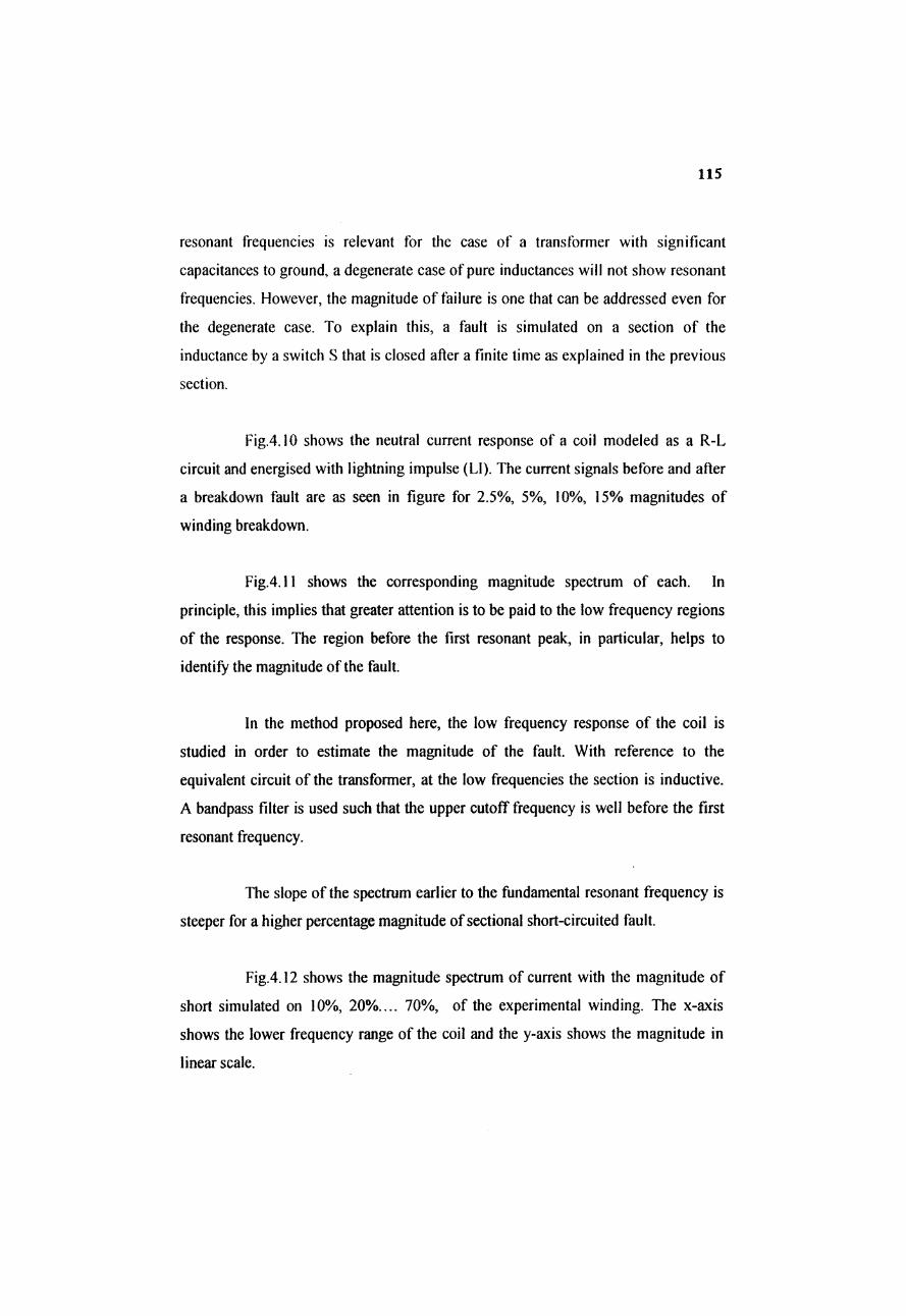
resonant frequencies is relevant for the case of a transformer with significant

capacitances to ground, a degenerate case of pure inductances will not show resonant

frequencies. However, the magnitude of failure is one that can be addressed even for

the degenerate case. To explain this, a fault is simulated on a section of the

inductance by a switch S that is closed after a finite time as explained in the previous

section.

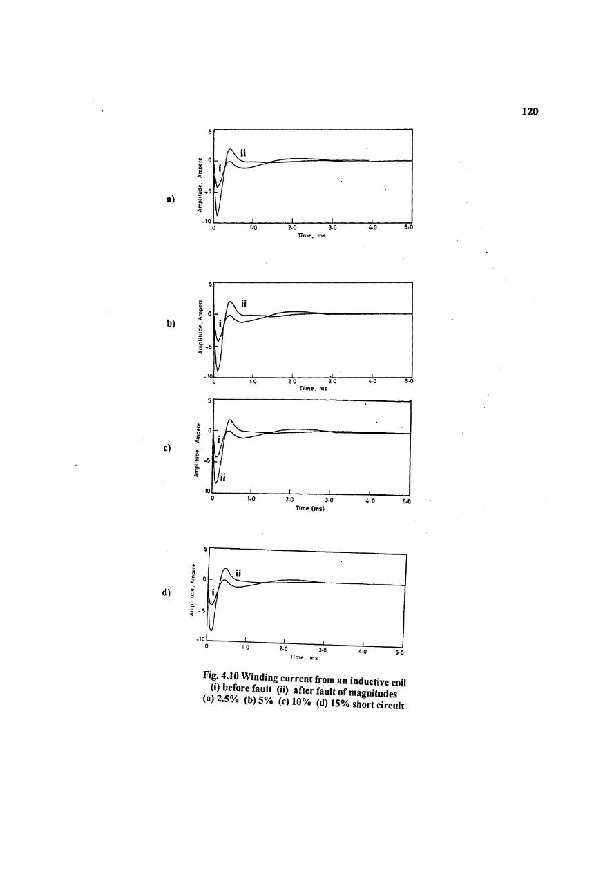
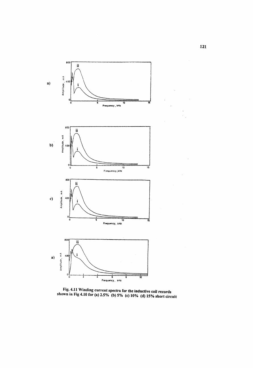
Fig.4.10 shows the neutral current response of a coil modeled as a R-L

circuit and energised with lightning impulse (LI). The current signals before and after

a breakdown fault are as seen in figure for 2.5%, 5%, 10%, 15% magnitudes of

winding breakdown.

Fig.4.11 shows the corresponding magnitude spectrum of each. In

principle, this implies that greater attention is to be paid to the low frequency regions

of the response. The region before the first resonant peak, in particular, helps to

identity the magnitude of the fault.

In the method proposed here, the low frequency response of the coil is

studied in order to estimate the magnitude of the fault. With reference to the

equivalent circuit of the transformer, at the low frequencies the section is inductive.

A bandpass filter is used such that the upper cutoff frequency is well before the first

resonant frequency.

The slope of the spectrum earlier to the fundamental resonant frequency is

steeper for a higher percentage magnitude of sectional short-circuited fault.

Fig.4.12 shows the magnitude spectrum of current with the magnitude of

short simulated on 10%, 20%.... 70%, of the experimental winding. The x-axis

shows the lower frequency range of the coil and the y-axis shows the magnitude in

linear scale.

UC

RP

cp

AV

R

Fig. 4.7a Pole variation response PVR (A) f, (B) f2 (C) f3

4.7b Amplitude variation response AVR (A) 10% (B) 20% (C)25%

Percentage of winding

Fig. 4.7c Uniform coil resonance parameter UCRP (A) 10% (B) 20% (C)30%

Fig. 4.7 Percentage variation of parameter

117

3 4Peak number

3 4Peak number

Fig.4.8 Relative variation of pole peak of resonant frequencies for similar fault at (a) Top (b) middle (c) ground end of winding

Freq

uenc

y, kHz

Freq

uenc

y, kHz

116

_____________ PERCENTILE LENGTH (x/l) ____________________

Fig.4.9b Pole variation response for an input of 1.2 /6 ps on a coil of a = 4

119

PERCENTILE LENGTH (x/l)

Fig.4.9d Pole variation response for an input of 1.2 /2 ps on a coil of a = 14

____________________________________ PERCENTILE LENGTH (xfl)

Fig.4.9c Pole variation response for an inpnt of 12750 ps on a coil of a = 4

-101-0 2-0 3-0

Tim* (ms)4-0 5-0

e C g; ”

B ^

OQ

o'»2 M

2 vO

Jm

0 1 ^ ^

s>

3 S 3

fit **■

a 2̂ o

as 5?

“» a

« 3 B

sr tS m

. O

OTP 5*

sal

2. = ?

• 2 O

- n

n n

nE. w o

£o

^ 3

£ CTQ

V)

<s /-s* e<2

N»

fljJD

VJ

(N

Am

plitu

de, A

mpe

re

800

ol------------------------ 1__________________ ' r i • i

0 2 4 6 t 10Frequency, kHz

Fig. 4.11 Winding current spectra for the inductive coil records shown in Fig 4.10 for (a) 2.5% (b)5% (c) 10% (d) 15% short circuit

10 15Frequency ,kHz

10Frequency, kHz

a)

Am

plitu

de, mA03

Am

plitu

de, m

AA

mpl

itude

, mA

122

A similar response is observed while simulating destructive faults on the

Abetti coil model and the result is as shown in Fig .4.13.

In all the above cases the amplitude of current spectrum before the first

resonant peak is indicative of the percentage magnitude of the fault.

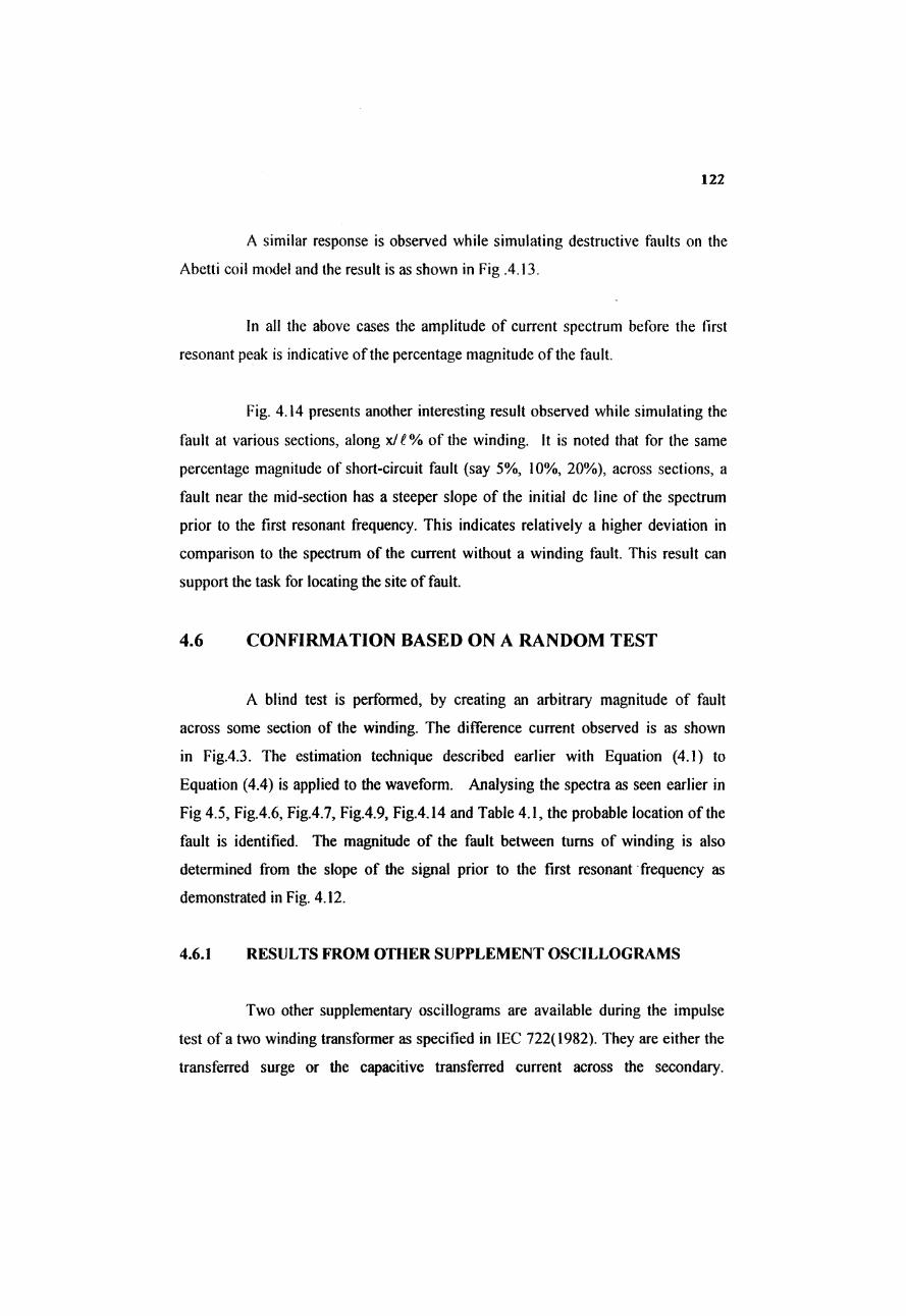
Fig. 4.14 presents another interesting result observed while simulating the

fault at various sections, along x/f% of the winding. It is noted that for the same

percentage magnitude of short-circuit fault (say 5%, 10%, 20%), across sections, a

fault near the mid-section has a steeper slope of the initial dc line of the spectrum

prior to the first resonant frequency. This indicates relatively a higher deviation in

comparison to the spectrum of the current without a winding fault. This result can

support the task for locating the site of fault.

4.6 CONFIRMATION BASED ON A RANDOM TEST

A blind test is performed, by creating an arbitrary magnitude of fault

across some section of the winding. The difference current observed is as shown

in Fig.4.3. The estimation technique described earlier with Equation (4.1) to

Equation (4.4) is applied to the waveform. Analysing the spectra as seen earlier in

Fig 4.5, Fig.4.6, Fig.4.7, Fig.4.9, Fig.4.14 and Table 4.1, the probable location of the

fault is identified. The magnitude of the fault between turns of winding is also

determined from the slope of the signal prior to the first resonant frequency as

demonstrated in Fig. 4.12.

4.6.1 RESULTS FROM OTHER SUPPLEMENT OSCILLOGRAMS

Two other supplementary oscillograms are available during the impulse

test of a two winding transformer as specified in IEC 722(1982). They are either the

transferred surge or the capacitive transferred current across the secondary.

123

Frequency, kHz

Frequency, kHz14-96

Fig. 4.12 Identification of magnitude of fault as a variation in slope before the first resonant frequency for the experimental coil

Abs

olut

e mag

nitu

de, volt

s

Fig. 4.13 Identification of magnitude of fault as a variation in slope before the first resonant frequency for the analytical coil

124

Frequency for 10*/« fault, Hz

Fig. 4.14 Identifying location of sectional fault from magnitude variation in slope of winding current

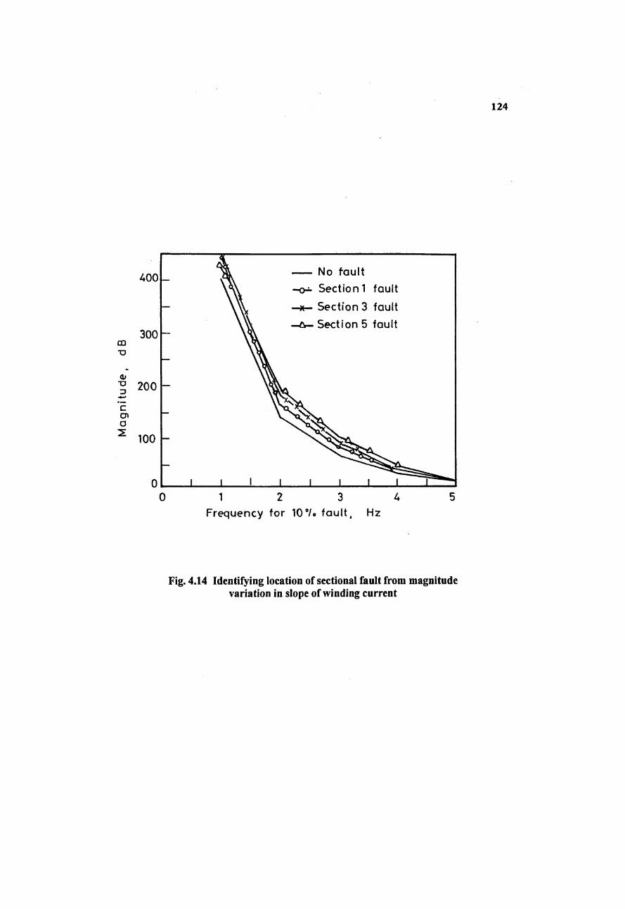
Fig.4.15 Signal records before occurrence of fault from neutral current methodand transferred surge method

a) Applied voltage V(t) b) Transferred surge output voltage Vwt(t)

c) Applied voltage V(t) d) Neutral winding curent iwt(t)

126

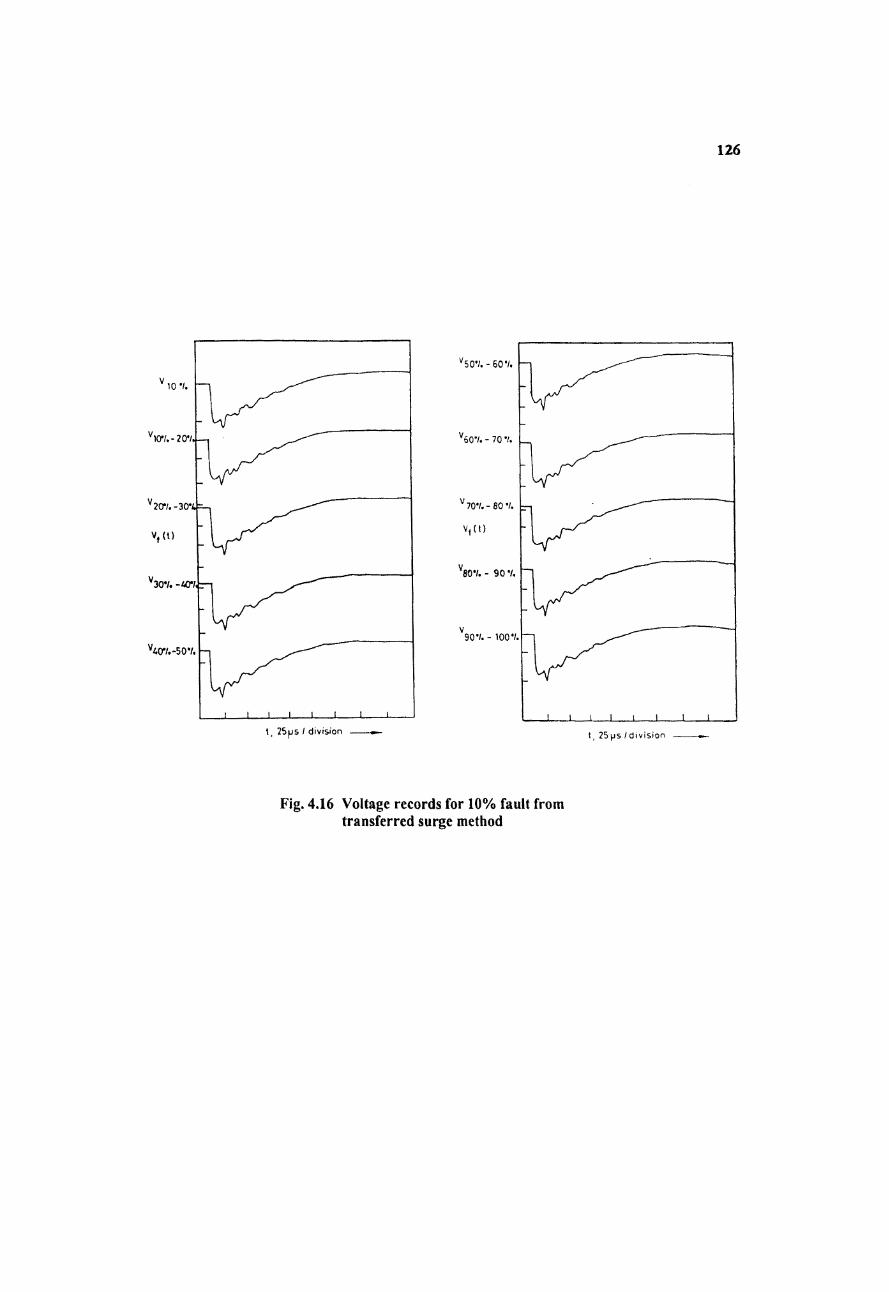
Fig. 4.16 Voltage records for 10% fault from transferred surge method

127

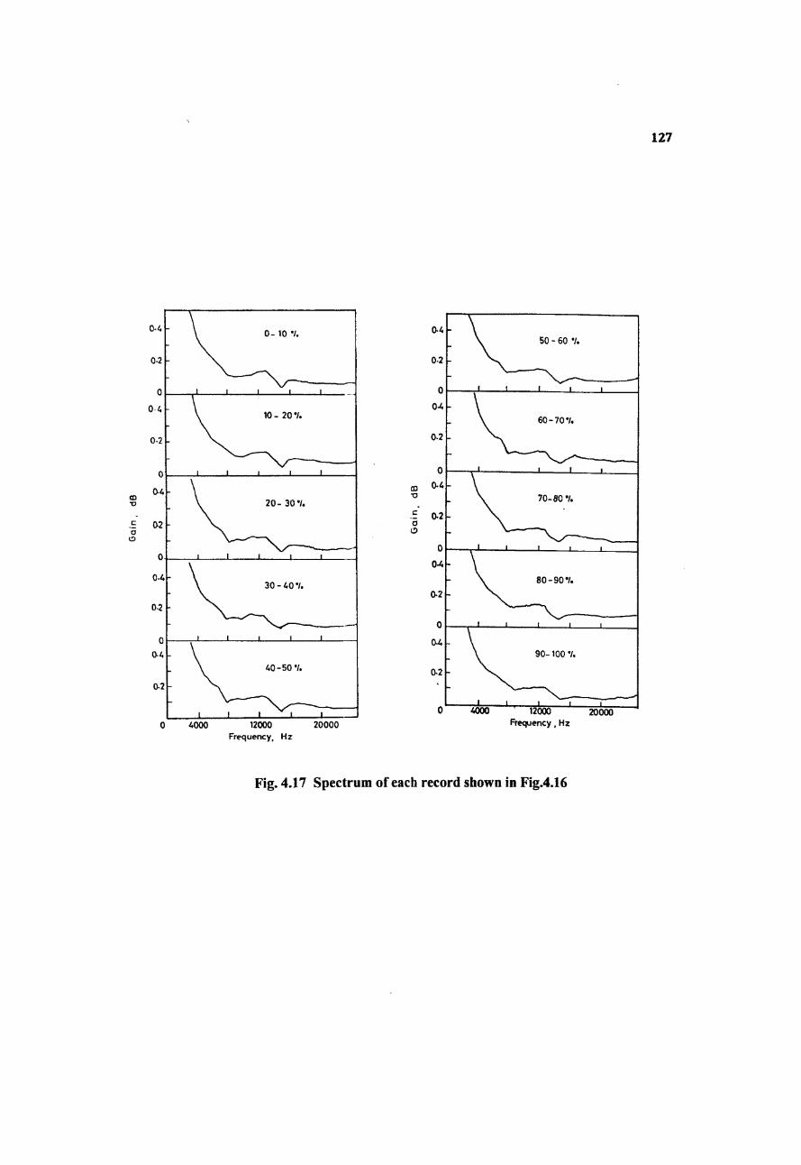
Fig. 4.17 Spectrum of each record shown in Fig.4.16

128

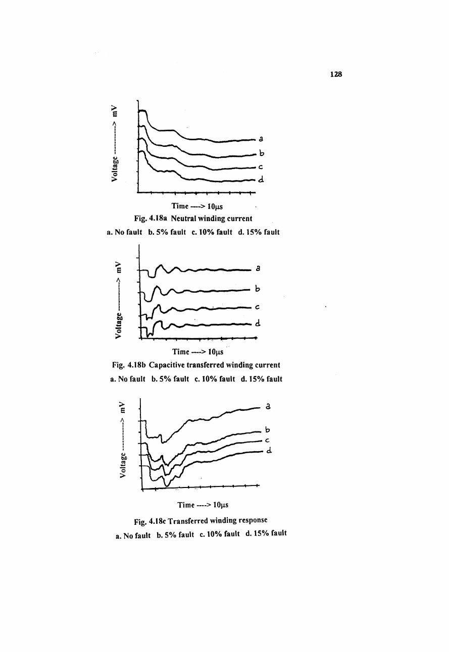
Time —> lOpsFig. 4.18b Capacitive transferred winding current

a. No fault b. 5% fault c. 10% fault d. 15% fault

.....1' i -..1................%... ...I..

Time —> lOpsFig. 4.18a Neutral winding current

a. No fault b. 5% fault c. 10% fault d. 15% fault

<0 _o

u

Vol

tage

------

---->

mVV

olta

ge---

------

-> mV

O tr

Vol

tage

------

---->

mV

Time —> lOps

Fig. 4.18c Transferred winding response a. No fault b. 5% fault c. 10% fault d. 15% fault

129

Frequency---- > 50 KHz

Fig. 4.19a Spectra of corresponding records in Fig. 4.18a

Frequency---- > 100 KHzFig. 4.19bSpectra of corresponding records in Fig. 4.18b

Frequency---- > 50 KHz

Fig. 4.19c Spectra of corresponding records in Fig. 4.18c

130

Experiments are also done to analyse the sensitivity of these two methods for fault

location.

Fig.4.15 shows typical records of voltage and winding current for the case

of the transferred voltage and the neutral current method of an unfaulted winding.

Fig.4.16 shows the records from transferred surge analysis for the experimental coil.

Fig.4.17 shows the corresponding spectra of each. However, the estimated

parameters with the neutral current are complementary to the results obtained from

the transferred surge method.

Fig.4.18 shows a sample of each of the experimental analysis using the

neutral current method, capacitive transferred surge method and transferred surge

voltage method. Fig. 4.19 shows the respective spectra for each of the records.

Similar characteristics in the estimated parameters are observed with

capacitive transferred current surge method and the transferred surge voltage method.

4.7 CONCLUSION

An attempt is made in proposing a method for the location of non-restoring

fault in transformer windings. The Abetti coil used here for simulation is a popularly

acknowledged model used in simulation studies. The results presented from

simulation and experimental study illustrate the above as a reliable method for

locating the site of defect and in detecting the magnitude of fault prior to untanking

of the transformer in test center.

Having established methods for location and identification of faults and

discharge, additional methods for fault location are possible using advanced time-

frequency (t-f) response analysis as discussed in the following chapter. Further, the

usefulness of the new t-f technique for an improved signal analysis in the presence of

noise is shown.