Chapter 4: Image Enhancement Introduction and Gray- Scale Modification

Chapter 4: Image Enhancement

Introduction and Gray-Scale Modification

Introduction

• Image enhancement techniques are used to emphasize and sharpen image features for display and analysis.

• In general, image enhancement is used to generate a visually desirable image.– It can be used as a preprocess or a

postprocess.– Highly application dependent. A technique

that works for one application may not work for another.

Introduction

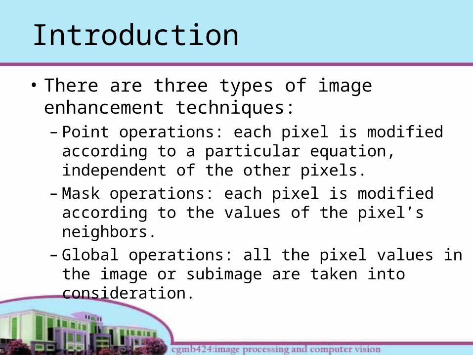
• There are three types of image enhancement techniques:– Point operations: each pixel is modified

according to a particular equation, independent of the other pixels.

– Mask operations: each pixel is modified according to the values of the pixel’s neighbors.

– Global operations: all the pixel values in the image or subimage are taken into consideration.

Overview of Gray-Scale Modification• Gray-scale modification methods belong

in the category of point operations.• They function by changing the pixel’s

gray-level value by using a mapping equation.– The mapping function maps the original

gray-level values to other, specified values.• The primary operations applied to the

gray scale of an image are to compress or stretch it.

Overview of Gray-Scale Modification• Gray-level compression is done to gray-

level ranges that are of little interest.• Gray-level stretching is done to gray-

level ranges where we desire more information.

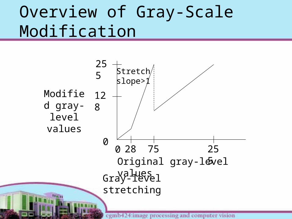
• The gray-level compression and stretching can be illustrate using the graph of modified gray-level vs. original gray-level.

Overview of Gray-Scale Modification

255

128

00 2557528Original gray-level values

Modified gray-level

values

Stretch slope>1

Gray-level stretching


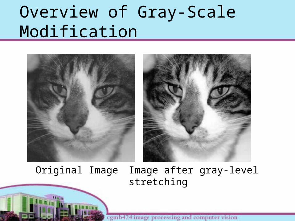
Original Image Image after gray-level stretching

Overview of Gray-Scale Modification• If the mapping line has a slope

between 0 and 1, this is called gray-level compression.

• If the slope is greater than one, then it is called gray-level stretching.

• In the previous example, the range of gray-level values from 28 to 75 is stretched, while other gray-level values are left alone.

Overview of Gray-Scale Modification• Stretching a particular gray-level range

can expose a previously hidden visual info.

• In some cases, we may want to stretch a specific range of gray levels, while clipping the values at the low and high ends.

• The effect of doing this is that the contrast of the image is enhanced.


255

128

00 25550

Original gray-level values

Modified gray-level

values

Gray-level stretching with clipping at ends

200


Original Image Image after gray-level stretching

Overview of Gray-Scale Modification• Another type of mapping equation is

called the intensity-level slicing.– Used for feature extraction.

• Here we select specific gray-level values of interest and map them to a specified, typically higher, value.

• Using this method, we can “bring out” the feature of interest in the image.




Histogram Modification

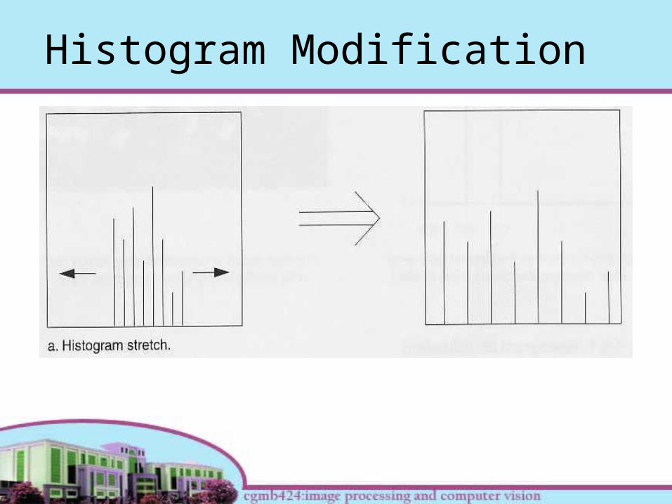
• An alternate perspective to gray-level modification that performs a similar function is referred to as histogram modification.

• The gray-level histogram of an image is the distribution of the gray levels in an image.

• The characteristics of an image can be determined from its histogram (refer to “Histogram Features” in Chapter 2).



• The histogram can be modified by a mapping function which will stretch, shrink or slide the histogram.– This will change the contrast or

brightness of the image.

• The graphical representation of histogram stretch, shrink and slide can be seen in the following diagrams.





• The mapping equation for histogram stretch can be found as follows:

MINMINMAXcrIcrI

crIcrIcrIStretch

MINMAX

MIN

),(),(

),(),()),((

I(r,c)MAX is the largest gray level value in the image I(r,c)I(r,c)MIN is the smallest gray level value in I(r,c)MAX and MIN correspond to the maximum and minimum gray-level values of the new range.


• This equation will take an image and stretch the histogram across the entire gray-level range.– This will increase the contrast of a low-

contrast image.

• If a stretch is desired over a smaller range, different MAX and MIN values can be specified.


Low-contrast image Histogram of low-contrast image


Image after histogram stretching Histogram of image after stretching


• If most of the pixel values in an image fall within a small range, but a few outliners force the histogram to span the entire range, a pure histogram stretch will not improve the image.

• In this case, it is useful to allow a small percentage of the pixel values to be clipped at the low and high end of the range.


Original Image Histogram of the original image


Image after histogram stretching without clipping

Histogram of the image


Image after histogram stretching with clipping 3% low and high value



• The opposite of histogram stretch is a histogram shrink, which will decrease image contrast by compressing the gray levels.

• The histogram shrinking equation is generally the same as the one for stretching.– But for histogram shrinking, MAX and MIN

should be set to the maximum and minimum of the new, compressed range.


Original image Histogram of original image


Image after histogram shrink to the range [75, 175]



• In general, histogram shrink reduces contrast and may not seem to be useful as image enhancement tool.

• However, there is an image-sharpening technique algorithm that uses the histogram shrink process as a part of the enhancement technique.


• The histogram slide technique can be used to make an image either darker or lighter.– Darker: slide histogram towards low end.– Lighter: slide histogram towards high end.

• Histogram slide is done by adding or subtracting a fixed number from all the gray-level values.

OFFSETcrIcrISlide ),()),((


• Any values slid past the minimum or maximum values will be clipped to the respective minimum and maximum.

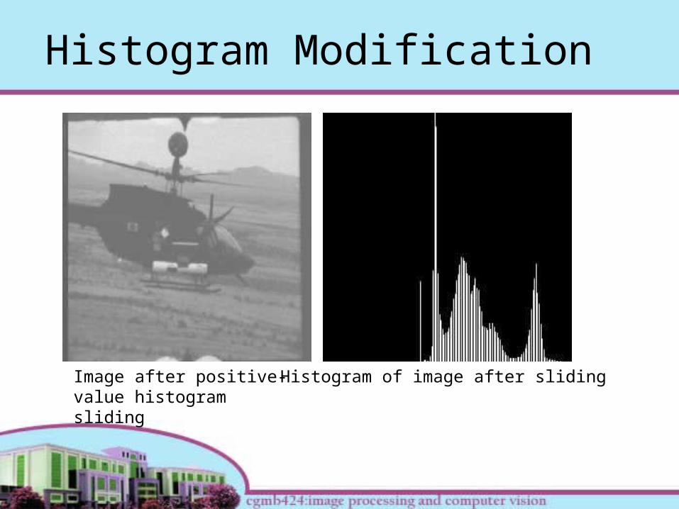
• A positive OFFSET will increase the overall brightness.

• A negative OFFSET will create a darker image.




Image after positive-value histogram sliding

Histogram of image after sliding


• Histogram equalization is a popular technique for improving the appearance of a poor image.

• Its function is similar to that of histogram stretch but often provides more visually pleasing results across a wider range of images.


• The histogram equalization process consists of four steps:– Find the running sum of the histogram

values.– Normalize the values from step 1 by

dividing by the total number of pixels.– Multiply the values from step 2 by the

maximum gray level value and round.– Map the gray-level values to the result

from step 3 using one-to-one correspondence.


• Example: You are given a 3 bits/pixel image with the following histogram:

• Next, perform the four steps histogram equalization process as mentioned before. The result can be seen in the tables in the next slide.

Gray-level 0 1 2 3 4 5 6 7

No of Pixel 10 8 9 2 14 1 5 2


Gray-level 0 1 2 3 4 5 6 7

No of Pixel 10 8 9 2 14 1 5 2

Run Sum 10 18 27 29 43 44 49 51

Normalized 10/51 18/51 27/51 29/51 43/51 44/51 49/51 51/51

Multiply by 7

1 2 4 4 6 6 7 7

Old 0 1 2 3 4 5 6 7

New 1 2 4 4 6 6 7 7

The first three steps:

The fourth step:




Image after histogram equalization

Histogram after equalization

Histogram Specification

• Sometimes, it is useful to be able to define a histogram and modify the histogram of the original image to match the histogram that we define.

• Such as process is called histogram specification.

• This process can be implemented in 4 steps:


– Find the mapping table to histogram-equalize the image (this is basically the result of histogram equalization).

– Specify the desired histogram.– Find the mapping table to histogram-equalize

the values of the desired histogram (this is done by applying histogram equalization to the specified histogram in step 2).

– Map the original values to the values from step 3.

Histogram SpecificationStep 1: Use histogram equalization result from last example

Original Gray-level Value - O 0 1 2 3 4 5 6 7

Histogram Equalized Values - H

1 2 4 4 6 6 7 7

Gray-Level Value 0 1 2 3 4 5 6 7

Number of Pixels in Desired Histogram

1 5 10 15 20 0 0 0

Step 2: Specify the desired histogram


Gray-Level Value 0 1 2 3 4 5 6 7

Histogram Equalized Values - S

0 1 2 4 7 7 7 7

Step 3: Find the histogram equalization mapping table for the desired histogram

O 0 1 2 3 4 5 6 7

H 1 2 4 4 6 6 7 7

S 0 1 2 4 7 7 7 7

M 1 2 3 3 4 4 4 4

Step 4: Map the original values to the values from step 3

Adaptive Contrast Enhancement

• Adaptive Contrast Enhancement (ACE) filter is used with an image with uneven contrast.– In this case, we want to adjust the contrast

differently in different regions of the image.– Regions with low contrast should be given more

contrast compared to other regions.

• This is different from image modification techniques, which are based only on global parameters.

Adaptive Contrast Enhancement• ACE works by using both the local

and global image statistics to determine the amount of contrast adjustment required.

• The image is processed using the sliding window concept.– The local image statistics are found by

considering only the current window.– The global statistics are found by

considering the entire image.


• The ACE equation is as follows:

– mI(r,c) = is the mean for the entire image I(r,c)

– σl = local standard deviation (in the window)

– ml = local mean (average in window)

– k1, k2 = constants, vary between 0 and 1

),(),(),(),( 2

),(1 crmkcrmcrI

cr

mkACE ll

l

crI

Adaptive Contrast Enhancement• This filter subtracts the local mean

from the original data and weights the result by the local gain factor k1[mI(r,c)/σl(r,c)].– This has the effect of intensifying local

variations.

– Can be controlled by the constant k1.

– Areas of low contrast (low values of σl(r,c)) are boosted.


• The mean is then added back to the result, weighted by k2 to restore the local average brightness.

• In practice, it is often helpful to shrink the histogram of image before applying this filter.

• It is also helpful to limit the range of the local gain factor, i.e. set a minimum and maximum for the local gain factor.


Original Image Histogram equalized version of original image


Image after being applied with ACE filter.k1 = 0.9, k2 = 0.5 Local gain max = 25

Histogram equalized version of ACE filtered image

Documents

Chapter 4: Image Enhancement Introduction and Gray- Scale Modification