Embed Size (px)
Citation preview

57:020 Fluid Mechanics Chapter 4 Professor Fred Stern Fall 2006 1
Chapter 4: Fluids Kinematics Velocity and Description Methods Primary dependent variable is fluid velocity vector V = V ( r ); where r is the position vector If V is known then pressure and forces can be determined using techniques to be discussed in subsequent chapters. Consideration of the velocity field alone is referred to as flow field kinematics in distinction from flow field dynamics (force considerations). Fluid mechanics and especially flow kinematics is a geometric subject and if one has a good understanding of the flow geometry then one knows a great deal about the solution to a fluid mechanics problem. Consider a simple flow situation, such as an airfoil in a wind tunnel:
kzjyixr ++=
ˆˆ ˆ( , )V r t ui vj wk= + +
x
r
U = constant

57:020 Fluid Mechanics Chapter 4 Professor Fred Stern Fall 2006 2
Velocity: Lagrangian and Eulerian Viewpoints There are two approaches to analyzing the velocity field: Lagrangian and Eulerian Lagrangian: keep track of individual fluids particles (i.e., solve F = Ma for each particle) Say particle p is at position r1(t1) and at position r2(t2) then,
kdtdzj
dtdyi
dtdx
ttrr
limV12
12
0tp ++=−
−=
→∆
= kwjviu ppp ++ Of course the motion of one particle is insufficient to describe the flow field, so the motion of all particles must be considered simultaneously which would be a very difficult task. Also, spatial gradients are not given directly. Thus, the Lagrangian approach is only used in special circumstances. Eulerian: focus attention on a fixed point in space
kzjyixx ++= In general, kwjviu)t,x(VV ++==
57:020 Fluid Mechanics Chapter 4 Professor Fred Stern Fall 2006 3
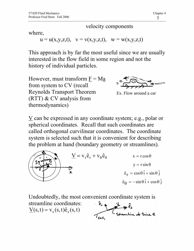
velocity components where, u = u(x,y,z,t), v = v(x,y,z,t), w = w(x,y,z,t) This approach is by far the most useful since we are usually interested in the flow field in some region and not the history of individual particles. However, must transform F = Ma from system to CV (recall Reynolds Transport Theorem (RTT) & CV analysis from thermodynamics) V can be expressed in any coordinate system; e.g., polar or spherical coordinates. Recall that such coordinates are called orthogonal curvilinear coordinates. The coordinate system is selected such that it is convenient for describing the problem at hand (boundary geometry or streamlines).
Undoubtedly, the most convenient coordinate system is streamline coordinates:
)t,s(e)t,s(v)t,s(V ss=
Ex. Flow around a car
θθ+= evevV rr
jcosisine
jsinicosre
sinry
cosrx
θ+θ−=θ
θ+θ=
θ=
θ=

57:020 Fluid Mechanics Chapter 4 Professor Fred Stern Fall 2006 4
However, usually V not known a priori and even if known streamlines maybe difficult to generate/determine. Streamlines, Streaklines, and Pathlines Streamlines is a line that is everywhere tangent to the velocity field. If the flow is steady, nothing at a fixed point (including the velocity direction) changes with time, so the streamlines are fixed lines in space. For unsteady flows the streamlines may change shape with time.
Streamlines are lines tangent to the velocity field.
As illustrated in the above figure, for two-dimensional flows the slope of the streamline, dy/dx, must be equal to the tangent of the angle that the velocity vector makes with the x axis or
dy vdx u
= If the velocity field is known as a function of x and y (and t if the flow is unsteady), this equation can be integrated to give the equation of the streamlines. A streakline consists of all particles in a flow that have previously passed through a common point. Streaklines are more of a laboratory tool than an analytical tool. They can be obtained by taking instantaneous photographs of marked

57:020 Fluid Mechanics Chapter 4 Professor Fred Stern Fall 2006 5
particles that all passed through a given location in the flow field at some earlier time. Such a line can be produced by continuously injecting marked fluid (neutrally buoyant smoke in air, or dye in water) at a given location.
(a) Flow past a full-sized streamlined vehicle in the GM aerodynamics laboratory wind tunnel, and 18-ft by 34-ft test section facility driven by a 4000-hp, 43-ft-diameter fan. (b) Surface flow on a model vehicle as indicated by tufts attached to the surface.

57:020 Fluid Mechanics Chapter 4 Professor Fred Stern Fall 2006 6
If the flow is steady, each successively injected particle follows precisely behind the previous one, forming a steady streakline that is exactly the same as the streamline through the injection point. For unsteady flows, particles injected at the same point at different times need not follow the same path. An instantaneous photograph of the marked fluid would show the streakline at that instant, but it would not necessarily coincide with the streamline through the point of injection at that particular time nor with the streamline through the same injection point at a different time A pathline is the line traced out by a given particle as it flows from one point to another. The pathline is a Lagrangian concept that can be produced in the laboratory by marking a fluid particle (dying a small fluid element) and taking a time exposure photograph of its motion.
Motion of water induced by surface waves

57:020 Fluid Mechanics Chapter 4 Professor Fred Stern Fall 2006 7
Acceleration Field and Material Derivative The acceleration of a fluid particle is the rate of change of its velocity. In the Lagrangian approach the velocity of a fluid particle is a function of time only since we have described its motion in terms of its position vector.
dtdw
adt
dva
dtdu
a
kajaiadt
rddtvd
a
kwjviudtrd
V
k)t(zj)t(yi)t(xr
pz
py
px
zyx2p
2p
p
pppp
p
pppp
===
++===
++==
++=
In the Eulerian approach the velocity is a function of both space and time; consequently,
k)t,z,y,x(wj)t,z,y,x(vi)t,z,y,x(uV ++=
ˆ ˆˆ ˆ ˆ ˆx y z
DV Du Dv Dwa i j k a i a j a kDt Dt Dt Dt
= = + + = + +
xDu u u x u y u z u u u ua u v wDt t x t y t z t t x y z
∂ ∂ ∂ ∂ ∂ ∂ ∂ ∂ ∂ ∂ ∂= = + + + = + + +
∂ ∂ ∂ ∂ ∂ ∂ ∂ ∂ ∂ ∂ ∂
called substantial derivative DtDu
x,y,z are f(t) since we must follow the particle in evaluating dV/dt
57:020 Fluid Mechanics Chapter 4 Professor Fred Stern Fall 2006 8
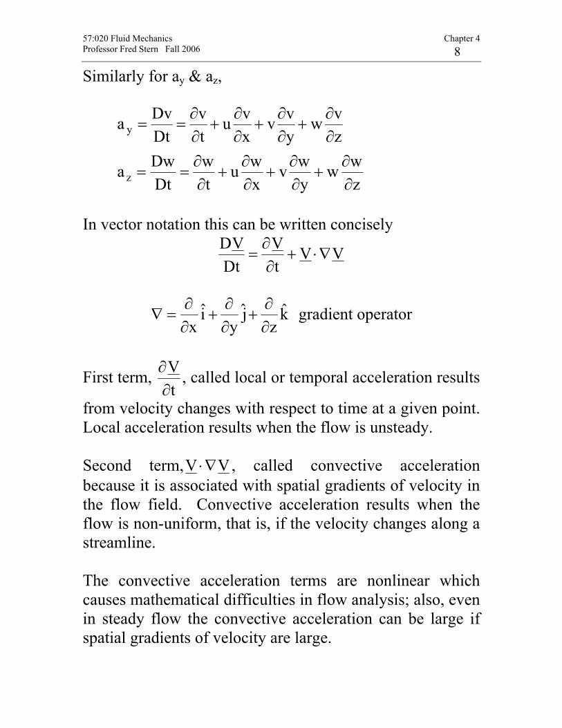
Similarly for ay & az,
zww
ywv
xwu
tw
DtDwa
zvw
yvv
xvu
tv
DtDva
z
y
∂∂
+∂∂
+∂∂
+∂∂
==
∂∂
+∂∂
+∂∂
+∂∂
==
In vector notation this can be written concisely
VVtV
DtVD
∇⋅+∂∂
=
kz
jy
ix ∂
∂+
∂∂
+∂∂
=∇ gradient operator
First term, tV∂∂ , called local or temporal acceleration results
from velocity changes with respect to time at a given point. Local acceleration results when the flow is unsteady. Second term, VV ∇⋅ , called convective acceleration because it is associated with spatial gradients of velocity in the flow field. Convective acceleration results when the flow is non-uniform, that is, if the velocity changes along a streamline. The convective acceleration terms are nonlinear which causes mathematical difficulties in flow analysis; also, even in steady flow the convective acceleration can be large if spatial gradients of velocity are large.
57:020 Fluid Mechanics Chapter 4 Professor Fred Stern Fall 2006 9
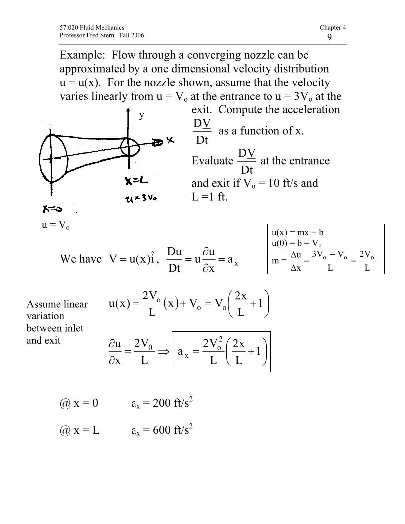
Example: Flow through a converging nozzle can be approximated by a one dimensional velocity distribution u = u(x). For the nozzle shown, assume that the velocity varies linearly from u = Vo at the entrance to u = 3Vo at the
exit. Compute the acceleration
DtVD as a function of x.
Evaluate Dt
VD at the entrance
and exit if Vo = 10 ft/s and L =1 ft.
We have i)x(uV = , xaxuu
DtDu
=∂∂
=
( ) ⎟⎠⎞
⎜⎝⎛ +=+= 1
Lx2VVx
LV2)x(u oo
o
⇒=∂∂
LV2
xu 0 ⎟
⎠⎞
⎜⎝⎛ += 1
Lx2
LV2a
2o
x
@ x = 0 ax = 200 ft/s2 @ x = L ax = 600 ft/s2
u = Vo
y
Assume linear variation between inlet and exit
u(x) = mx + b u(0) = b = Vo
m = LV2
LVV3
xu ooo =
−=
∆∆

57:020 Fluid Mechanics Chapter 4 Professor Fred Stern Fall 2006 10
Separation, Vortices, Turbulence, and Flow Classification We will take this opportunity and expand on the material provided in the text to give a general discussion of fluid flow classifications and terminology. 1. One-, Two-, and Three-dimensional Flow
1D: V = i)y(u 2D: V = j)y,x(vi)y,x(u + 3D: V = V(x) = k)z,y,x(wj)z,y,x(vi)z,y,x(u ++
2. Steady vs. Unsteady Flow
V = V(x,t) unsteady flow V = V(x) steady flow
3. Incompressible and Compressible Flow
0DtD
=ρ ⇒ incompressible flow
representative velocity
Ma = cV
speed of sound in fluid

57:020 Fluid Mechanics Chapter 4 Professor Fred Stern Fall 2006 11
Ma < .3 incompressible Ma > .3 compressible Ma = 1 sonic (commercial aircraft Ma∼.8) Ma > 1 supersonic
Ma is the most important nondimensional parameter for compressible flow (Chapter 7 Dimensional Analysis)
4. Viscous and Inviscid Flows
Inviscid flow: neglect µ, which simplifies analysis but (µ = 0) must decide when this is a good
approximation (D’ Alembert paradox body in steady motion CD = 0!)
Viscous flow: retain µ, i.e., “Real-Flow Theory” more (µ ≠ 0) complex analysis, but often no choice
5. Rotational vs. Irrotational Flow
Ω = ∇ × V ≠ 0 rotational flow Ω = 0 irrotational flow
Generation of vorticity usually is the result of viscosity ∴ viscous flows are always rotational, whereas inviscid flows

57:020 Fluid Mechanics Chapter 4 Professor Fred Stern Fall 2006 12
are usually irrotational. Inviscid, irrotational, incompressible flow is referred to as ideal-flow theory. 6. Laminar vs. Turbulent Viscous Flows
Laminar flow = smooth orderly motion composed of thin sheets (i.e., laminas) gliding smoothly over each other Turbulent flow = disorderly high frequency fluctuations superimposed on main motion. Fluctuations are visible as eddies which continuously mix, i.e., combine and disintegrate (average size is referred to as the scale of turbulence). Reynolds decomposition )t(uuu ′+= mean turbulent fluctuation motion usually u′∼(.01-.1)u , but influence is as if µ increased by 100-10,000 or more.

57:020 Fluid Mechanics Chapter 4 Professor Fred Stern Fall 2006 13
Example: Pipe Flow (Chapter 8 = Flow in Conduits) Laminar flow:
⎟⎠⎞
⎜⎝⎛−
µ−
=dxdp
4rR)r(u
22
u(y),velocity profile in a paraboloid
Turbulent flow: fuller profile due to turbulent mixing extremely complex fluid motion that defies closed form analysis.
Turbulent flow is the most important area of motion fluid dynamics research. The most important nondimensional number for describing fluid motion is the Reynolds number (Chapter 8)
Re = ν
=µρ VDVD V = characteristic velocity
D = characteristic length

57:020 Fluid Mechanics Chapter 4 Professor Fred Stern Fall 2006 14
For pipe flow V = V = average velocity D = pipe diameter Re < 2300 laminar flow Re > 2300 turbulent flow Also depends on roughness, free-stream turbulence, etc. 7. Internal vs. External Flows
Internal flows = completely wall bounded; Usually requires viscous analysis, except near entrance (Chapter 8) External flows = unbounded; i.e., at some distance from body or wall flow is uniform (Chapter 9, Surface Resistance) External Flow exhibits flow-field regions such that both inviscid and viscous analysis can be used depending on the body shape and Re.

57:020 Fluid Mechanics Chapter 4 Professor Fred Stern Fall 2006 15
Flow Field Regions (high Re flows)
Important features:
1) low Re viscous effects important throughout entire fluid domain: creeping motion
2) high Re flow about streamlined body viscous effects confined to narrow region: boundary layer and wake
3) high Re flow about bluff bodies: in regions of adverse pressure gradient flow is susceptible to separation and viscous-inviscid interaction is important
8. Separated vs. Unseparated Flow
Flow remains attached Streamlined body w/o separation
Bluff body Flow separates and creates
the region of reverse flow, i.e. separation
forceviscousforceinertiaVcRe =
ν=

57:020 Fluid Mechanics Chapter 4 Professor Fred Stern Fall 2006 16
Basic Control-Volume Approach and RTT

57:020 Fluid Mechanics Chapter 4 Professor Fred Stern Fall 2006 17

57:020 Fluid Mechanics Chapter 4 Professor Fred Stern Fall 2006 18
Reynolds Transport Theorem (RTT) Need relationship between ( )sysB
dtd and changes in
∫ ∀=∫=CVCV
ddmcvB βρβ .
1 = time rate of change of B in CV = ∫ ∀=CV
ddtd
dtcvdB
βρ
2 = net outflux of B from CV across CS =
RCS
V n DAβρ ⋅∫
SYS
RCV CS
dB d d V n dAdt dt
βρ βρ= ∀+ ⋅∫ ∫
General form RTT for moving deforming control volume
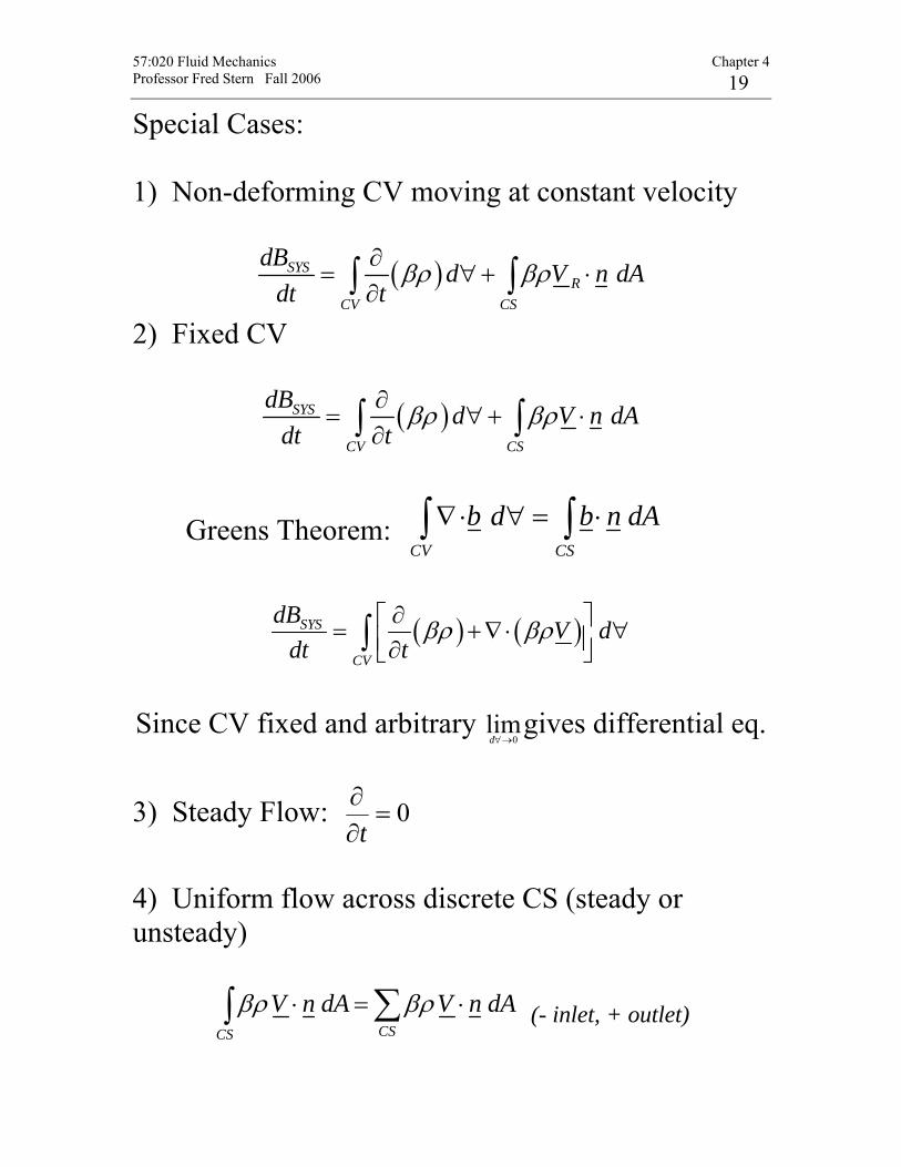
57:020 Fluid Mechanics Chapter 4 Professor Fred Stern Fall 2006 19
Special Cases: 1) Non-deforming CV moving at constant velocity
( )SYSR
CV CS
dB d V n dAdt t
βρ βρ∂= ∀+ ⋅
∂∫ ∫
2) Fixed CV
( )SYS
CV CS
dB d V n dAdt t
βρ βρ∂= ∀+ ⋅
∂∫ ∫
Greens Theorem: CV CS
b d b n dA∇⋅ ∀ = ⋅∫ ∫
( ) ( )SYS
CV
dB V ddt t
βρ βρ∂⎡ ⎤= +∇⋅ ∀⎢ ⎥∂⎣ ⎦∫
Since CV fixed and arbitrary
0lim
→∀dgives differential eq.
3) Steady Flow: 0=
∂∂t
4) Uniform flow across discrete CS (steady or unsteady)
CSCS
V n dA V n dAβρ βρ⋅ = ⋅∑∫ (- inlet, + outlet)
57:020 Fluid Mechanics Chapter 4 Professor Fred Stern Fall 2006 20
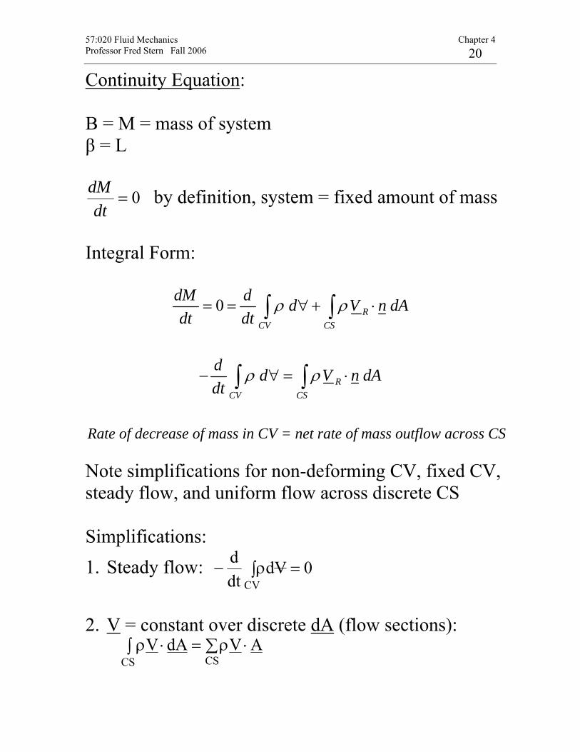
Continuity Equation: B = M = mass of system β = L
0=dt
dM by definition, system = fixed amount of mass
Integral Form:
0 RCV CS
dM d d V n dAdt dt
ρ ρ= = ∀+ ⋅∫ ∫
RCV CS
d d V n dAdt
ρ ρ− ∀ = ⋅∫ ∫
Rate of decrease of mass in CV = net rate of mass outflow across CS
Note simplifications for non-deforming CV, fixed CV, steady flow, and uniform flow across discrete CS Simplifications: 1. Steady flow: 0Vd
dtd
CV=∫ρ−
2. V = constant over discrete dA (flow sections):
∫ ∑ ⋅ρ=⋅ρCS CS
AVdAV
57:020 Fluid Mechanics Chapter 4 Professor Fred Stern Fall 2006 21
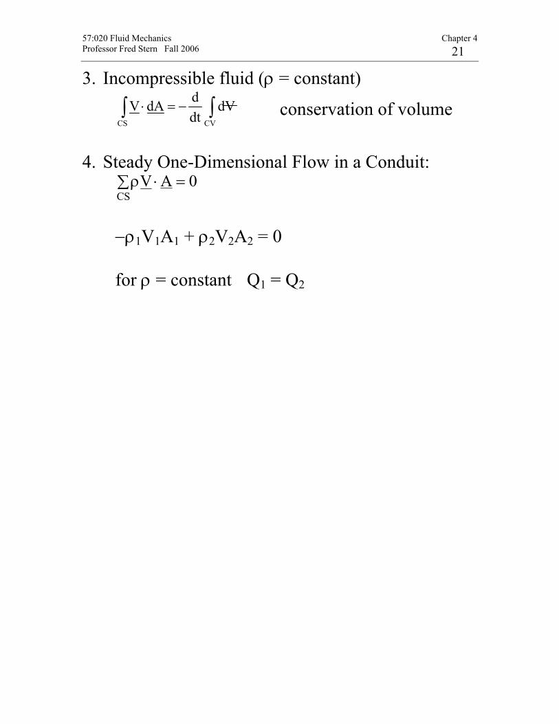
3. Incompressible fluid (ρ = constant)
CS CV
dV dA dVdt
⋅ = −∫ ∫ conservation of volume
4. Steady One-Dimensional Flow in a Conduit:
∑ =⋅ρCS
0AV
−ρ1V1A1 + ρ2V2A2 = 0 for ρ = constant Q1 = Q2