Chapter 4Continuous Random Variables and their Probability Distributions

Another one of life’s great adventures is about to begin.

Chapter 4A

The Road Ahead

today

+ special bonus – the triangular distribution!

Continuous Random Variables

Experiments and tests can result in values that are spread over a continuum.

Even if our measurement device has discrete values, it is often impractical to use a discrete distribution because the number of allowed values is so large.

We gain modeling flexibility by expanding the distributions available to us.

Measured values can be represented as R.V.’s Range of values is an interval of real numbers An ‘infinite’ number of outcomes are possible A Probability Density Function (pdf), f(x), is used to

describe the probability distribution of a continuous R.V., X.

Continuous Random Variables - Examples

T = a continuous random variable, time to failure X = a continuous random variable, the distance in miles

between cable defects Z = a continuous random variable, the monthly

consumption of power in watts T = a continuous random variable, the repair time of a

failed machine Y = a continuous random variable, the time between

arrivals of customers at City National Bank X = a continuous random variable, the procurement

lead-time for a critical part

4-2 Probability Distributions and Probability Density Functions

Definition

Probability Density Function

Fig 4.2 – Probability is determined from area under f(x).

area = 1

4-2 Probability Distributions and Probability Density Functions

Figure 4-3 Histogram approximates a probability density function.

Continuous Random Variables

Special Message Box:If X is a continuous R.V., P(X = x) = 0 (very important idea)There are an infinite number of points on the X-axis under the curve, the probability that the R.V., X, takes on any particular value, P(X = x), is zero.

Our First Example

Example 4-2

4-2 Probability Distributions and Probability Density Functions

Figure 4-5 Probability density function for Example 4-2.

4-2 Probability Distributions and Probability Density Functions

Example 4-2 (continued)

Our Very next Example

Given the PDF:

( ) , 0xf x e x

0 0

1lim 1

1 1

xx x

x

ee dx e

More of Our Very next Example

Given the PDF:

1. P(X > 1)

2. P(1 < X < 2.5)

3. P(X = 3)

4. P(X < 4)

( ) , 0xf x e x 1

1 1

.36791

xx e

e dx e

2.52.52.5 1

1 1

.28581

xx e

e dx e e

3

3

0xe dx 44

4 0

0 0

.98171

xx e

e dx e e

4-3 Cumulative Distribution Functions

Definition

4-3 Cumulative Distribution Functions

Example 4-4

4-3 Cumulative Distribution Functions

Figure 4-7 Cumulative distribution function for Example 4-4.

Given the CDF, find the PDF

( )( ) or ( ) ( )

xdF xf x F x f u du

dx

I can do this.

( ) 1 , 0

1( )( )

x

x

x

F x e x

d edF xf x e

dx dx

Cumulative Distribution Functions

( ) 0.05, 0 20

0, x < 0

( ) 0.05 , 0 x 20

1, 20 x

f x x

F x x

Figures 4-4 and 4-6 the PDF and CDF

The relation of these shapes ought to become intuitive to

you.

Problem 4-11

Suppose F(x) = .2x for 0 < x < 5, and F(x) = 1 for x > 5. F(x) = 0 otherwise.

Determine the following:

a. P(X < 2.8)

b. P(X > 1.5)

c. P(X < -2)

d. P(X > 6)

= F(2.8) = (.2)(2.8) = .56

= 1 - F(1.5) = 1 - (.2)(1.5) = .7

= F(-2) = 0

= 1 – F(6) = 1 – 1 = 0

A CDF Problem

Determine the CDF for f(x) =1.5x2, for –1 < x < 1

2 3 3

11

( ) ( ) ( )

1.5 = 1.5 0.5 0.5

3

x

x x

F x P X x f u du

u du u x

3

0, x 1

( ) 0.5 0.5, -1 1

1, 1

F x x x

x

PDF & CDF

f(x) – PDF –> 1.5x2

F(X)

0.0

0.2

0.4

0.6

0.8

1.0

1.2

-1-0

.8-0

.6-0

.4-0

.2 00.

20.

40.

60.

8 1

F(X)

0.0

0.2

0.4

0.6

0.8

1.0

1.2

1.4

1.6

f(x)

F(x) – CDF -> .5x3 + .5

4-4 Mean and Variance of a Continuous Random Variable

Definition

A Complete Example

Let X = a continuous random variable, the time to complete a complex task in hours.

The CDF is given by the following where b, the distribution parameter, is in hours:

2

( ) 1 1 ; 0x

F x x bb

2

( ) 1 2 2 2( ) 2 1 1

dF x x x xf x

dx b b b b b b

then

Let’s Graph the PDF and CDF

f(x)

0

0.05

0.1

0.15

0.2

0.25

0 2 4 6 8 10 12

x

F(x)

0

0.2

0.4

0.6

0.8

1

1.2

0 2 4 6 8 10 12

x

b = 10

Let’s find some probabilities

2

10

5Pr{ 5} (5) 1 1 .75

10

b

X F

2 25 2

Pr{2 5} (5) (2) 1 1 1 110 10

.75 .36 .39

X F F

27

Pr{ 7} 1 (7) 1 1 1 .0910

X F

More of a complete example

2 3

2 20 0

2 2 2 2 1[ ]

3 3 3

bb x x xE X x dx b b b

b b b b

3 42 2 2 2 2

2 20 0

22 2 2 2 2

2

2 2 2 2 1 1[ ]

3 2 3 2 6

1 1 1[ ] [ ] [ ]

6 3 18

1.2357

18

bb x x xE X x dx b b b

b b b b

Var X E X E X b b b

b b

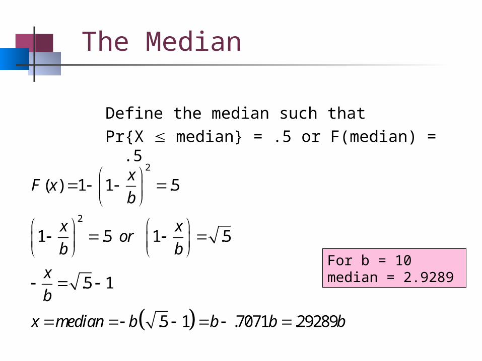
The Median

Define the median such that Pr{X median} = .5 or F(median) = .5

2

2

( ) 1 1 .5

1 .5 1 .5

.5 1

.5 1 .7071 .29289

xF x

b

x xor

b b

x

b

x median b b b b

For b = 10median = 2.9289

4-4 Mean and Variance of a Continuous Random Variable

Expected Value of a Function of a Continuous Random Variable

Note for continuous RV:E[a + bX] = a + b E[X]Var[a + bX] = b2 Var[X]

More of the Example

The cost for completing the task in the previous example is $50 times the square root of the task time. What is the expected cost of completing the task if b = 10 hours.

10

20

1010 .5 1.5 1.5 2.5

2 20 0

1.5 2.5

2

2 250 50

10 10

2 2 2 250 50

10 10 1.5 10 2.5 10

2 10 2 1050 $84.33

1.5 10 2.5 10

xE x x dx

x x x xdx

Observe:

10$50 50 $91.29

3

Problem 4-29

The thickness of a conductive coating in micrometers has a density function of 600x-2 for 100m < x < 120 m

(a) Find the mean and variance(b) If the coating cost $.50 per m of thickness on each part,

what is the average cost of the coating per part?

120120

2 100100

120 21202

2 100100

2

600[ ] 600ln 109.39293

600[ ] 600 12,000

[ ] 12,000 109.39293 33.186

xE X dx x

x

xE X dx x

x

V X

(b) E[cost] = .50 (109.34) = 54.70

Begin the Bonus Round

He is really going to do it -

discuss the triangular

distribution!

The Right Triangular Distribution

A continuous random variable is said to have a right triangular distribution if its density function is given by:

x

f(x)

b

( ) ; 0f x k x x b Find the value of k that makes f(x) a PDF:

0

2 2

0

2 2

1

12 2

2 2; ( ) 0

b

b

kx dx

kx kb

xk f x x b

b b

More Right Triangular Distribution

Now find the CDF and the mean of a right triangular distribution.

2

2 2

2 2 20 0

2 3 3

2 2 20 0

2( ) 0

2( )

2 2 2 2[ ]

3 3 3

xx

bb

xf x x b

b

y y xF x dy

b b b

x x bE X dx b

b b b

More Right Triangular Distribution

Now find the median of a right triangular distribution.

2

2

2

2

2( ) 0

( ) .5

.5 .7071

xf x x b

b

xF x

b

x b b

The Left Triangular Distribution

Big bonus 35

2 2( ) ; 0

2

af t a t t

a

a

t2/a

Please professor.

Can we students work this

one?

The General Triangular Distribution

Often used as a “rough” model in the absence of data. a – optimistic value b – pessimistic value c – most likely value (mode)

Bigger bonus

2

2( )

0

x aif a x c

b a c a

b xf x if c x b

b a b c

otherwise

a c b

f(x)

a < c < b

The General Triangular Distribution

It says here that the overachieving student will

explore these distributions in detail by finding the CDF,

mean, and median.

An overachievingstudent

Today’s discussion on continuous random variables has concluded

Say it isn’t so.