Chapter 4: Continuous Distributions 4.0 Continuous ...dspace.mit.edu/bitstream/handle/1721.1/66488/7-89-fall-2007/... · continuous and discrete distributions is that summing in discrete

Chapter 4: Continuous Distributions

4.0 Continuous Distributions

In the previous sections, we described cases where we could count the number of

discrete events that took place and described them with the distributions such as the

binomial, multinomial, or Poisson. However, in many cases we either cannot directly

count the number of events taking place or that number is too large to be practical. In

other cases, variables such as the time, length, and weight are naturally continuous rather

than discrete. Therefore we need a different kind of probability model to describe these

situations.

Fortunately, there exist a large family of continuous functions that lend

themselves to describe probability distributions. In some cases, these distributions are

just continuous analogs of discrete distributions, while in other cases the distributions are

empirical, and as such based only on data. Operationally, a key difference between

continuous and discrete distributions is that summing in discrete distributions is done

with sums, while summing a continuous distribution means integrating. By allowing us

to use the tools of calculus, continuous distributions provide many advantages not

available to discrete distributions.

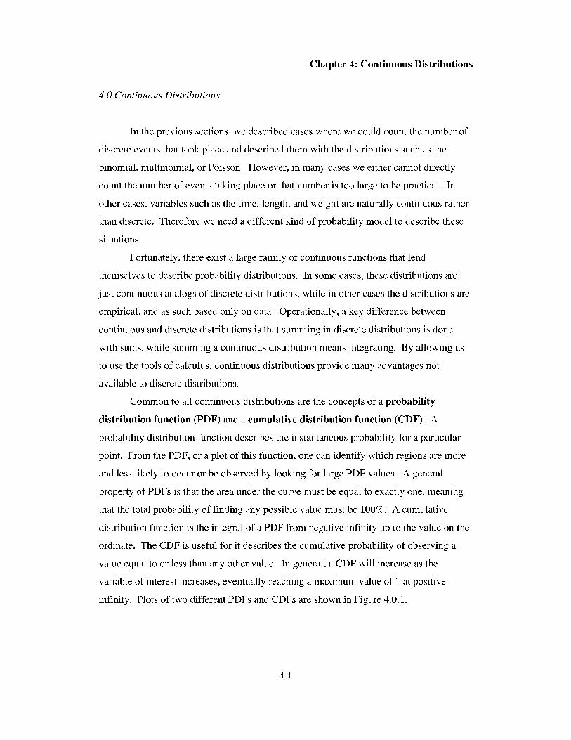
Common to all continuous distributions are the concepts of a probability

distribution function (PDF) and a cumulative distribution function (CDF). A

probability distribution function describes the instantaneous probability for a particular

point. From the PDF, or a plot of this function, one can identify which regions are more

and less likely to occur or be observed by looking for large PDF values. A general

property of PDFs is that the area under the curve must be equal to exactly one, meaning

that the total probability of finding any possible value must be 100%. A cumulative

distribution function is the integral of a PDF from negative infinity up to the value on the

ordinate. The CDF is useful for it describes the cumulative probability of observing a

value equal to or less than any other value. In general, a CDF will increase as the

variable of interest increases, eventually reaching a maximum value of 1 at positive

infinity. Plots of two different PDFs and CDFs are shown in Figure 4.0.1.


(a) PDF 1

0.35

0.3 1 P(r) 0.25 I

0.2 1

I 0.1

0.05

5 10 15 20

( c ) PDF 2

0.175

P(x) 0.125 t

0.05

0.025 ,! \\

1 0 20 3 1) 40

l , (b) CDF 1 ,7

(d) CDF2

0.8 . 0.8 .

( P ( X ) ~ . ~ . / JP(x) U6

0.4 . 0.4 .

i / 0.1 . 0 2 .

i I i' l-

5 1 U 15 20 1U 20 30 40

Figure 4.0.1 : Plots of the probability distribution function, (a) and (c), and cumulative

distribution function, (b) and (d) for two different distributions.

In this chapter we will show some of the more common continuous distributions,

where they come from, and how they are used in computational biology.

4.1 Gaussian Distribution

The Gaussian distribution, or Normal distribution, is probably the most

commonly encountered continuous distribution. Each time you take a set of data,

average it and calculate the standard deviation of that data, one implicitly assumes that

the underlying distribution is Gaussian.

The analytical expression of the Gaussian distribution can derived from the

binomial distribution using the De Moivre-Laplace theorem. The proof of this

relationship is lengthy, and as such we direct the interested reader to the original work by

Uspensky (1937) listed at the end of this chapter. The result of this calculation is an

analytical expression of the Gaussian distribution


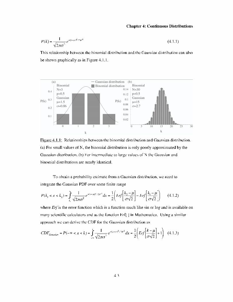
This relationship between the binomial distribution and the Gaussian distribution can also

be shown graphically as in Figure 4.1.1.

(a) - Gaussian distribution (b)

k k

Figure 4.1.1 : Relationships between the binomial distribution and Gaussian distribution.

(a) For small values of N, the binomial distribution is only poorly approximated by the

Gaussian distribution. (b) For intermediate to large values of N the Gaussian and

binomial distributions are nearly identical.

To obtain a probability estimate from a Gaussian distribution, we need to

integrate the Gaussian PDF over some finite range

where Eg i s the error function which is a function much like sin or log and is available on

many scientific calculators and as the function Erf[ ] in Mathematica. Using a similar

approach we can derive the CDF for the Gaussian distribution as


Example 4.1 .l: Weighing mice

We are interested in the weight of a particular mouse, yet we have only crude

scales with which to weigh the mouse. After trying out many scales, we obtain an

average weight of 16 grams with a standard deviation of 3 grams. From this data, what is

the probability that the mouse actually weighs more than 20 grams?

Solution

One approach to solve this problem is to assume that the underlying distribution

of the measurements is Gaussian and integrate. Using the expression in Equation 4.4

above, we find

P(201x<m)= d2:(3)2 e-(x-16)2 1 2 ( 3 ) ~ = ( E l - [ I ) = 0.092 2

Thus, there is a 9.12% chance that the mouse actually weighs more than 20 grams.

Note that we assumed that the underlying distribution was Gaussian when we

calculate a mean and standard deviation, but this approximation is not always accurate.

For example, here a Gaussian distribution also predicts that there is a 0.000004% chance

that the mouse could actually have a negative weight. Therefore, be aware that the

Gaussian distribution is not always the best choice for a distribution.

Example 4.1.2: Boron in plants

The healthy range of boron concentrations in most plant leaves ranges from 25 to

200 ppm. Beyond this range, most plants become stunted or sick. A random sample of

100 plants yields a symmetric distribution of readings, centered at 40 ppm with a

standard deviation of 10 ppm. From this sample, what percentage of plants likely suffers

from a boron deficiency?

Solution

The boron measurement in this problem is a continuous value and the distribution

is symmetric, therefore we will model boron concentrations as a Gaussian distribution.

To find the percent of plants that are boron deficient, we can directly use the Gaussian

CDF


2 CDF,,,,,, = P(-00 < x < 25) =

Thus, -7% of the plants likely suffer a boron deficiency. Note that the CDF integrates

from minus infinity to 25, while ppm measurements only go as low as zero. If we had

used the more general form of the CDF in 4.1.2, and integrated from 0 to 25 we would

have obtained a probability score of 0.06678, which is nearly identical to the CDF result.

4.2 Standard normal distribution and z-scores

A special case of the Gaussian distribution is one that is centered at zero (p=O)

with a standard deviation of exactly one (o=l). This distribution is called the standard

normal distribution, and provides a standardized way to discuss Gaussian distributions.

Given a standard normal distribution, the distance from the origin is measured by the

variable z, which is also called a z-score. The z-score is convenient because it is a single

number that can be related to any non-standard normal distribution through the following

transformation

Tables in statistics textbooks often have pre-calculated tables that show how the z-score

varies with the probability density.

Historically, the z-score was used in place of exact calculations using complicated

functions such as the error function shown in 4.1.2, however the concept is still useful for

making quick estimates. For example, if given the mean and standard deviation of a

normally distributed sample, one can easily determine the range of values that encompass

90%, 95%, and 99% of the probability density by using z-values of 1.645, 1.960, and

2.575 respectively. Other z-score values can be looked up in most statistics textbooks or

calculated using the CDF in equation 4.1.3.

Example 4.2.1: E. coli doubling times

After running repeated experiments, we find that the doubling time for a

particular strain of E. coli is 58 minutes with a standard deviation of 10 minutes. Using


z-scores, determine the range of expected doubling times at the 90% and 99% confidence

levels.

Solution

We start by rearranging the definition of the z-score transform in equation 4.2.1 to

solve for x

x,l,,l,, = C1+ z o xZollw = ,u - z o

Here we provide both the upper and lower limit by symmetrically adding or subtracting

from the mean. To find the upper limit of the 90% confidence interval we plug in a z-

value of 1.645 to yield

x,,,, = 58 + 1.645(10) = 74.45 min

x ,,,, = 58 - 1.645(10) = 41.55 min

At the 99% confidence interval we use a z-score of 2,575

x, ,,, = 58 + 2.575(10) = 83.75 min

x ,,,, = 58 - 2.575(10) = 32.25 min

From this calculation we are 95% sure that the doubling times will take between 41.55

and 74,45 minutes, and 99% sure that they will take place between 32,35 and 83.75

minutes.

4.3 Exponential distribution

When modeling the waiting time between successive changes, such as cell

differentiation or DNA mutations, or the distance between successive events, such as the

distance between simple repeats along the genome, one often uses the exponential

distribution. The exponential distribution has the following probability distribution

function

P ( x ) = A.e-h (4.3.1)

The cumulative distribution function for the exponential distribution function has the

form

CDFcxp(x) = 1 - e-h (4.3.2)


where A is the unit rate of change.

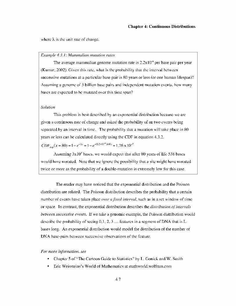
Example 4.3.1: Mammalian mutation rates

The average mammalian genome mutation rate is 2.2~10-' per base pair per year

(Kumar, 2002). Given this rate, what is the probability that the interval between

successive mutations at a particular base pair is 80 years or less (or one human lifespan)?

Assuming a genome of 3 billion base pairs and independent mutation events, how many

bases are expected to be mutated over this time span?

Solution

This problem is best described by an exponential distribution because we are

given a continuous rate of change and asked the probability of an two events being

separated by an interval in time. The probability that a mutation will take place in 80

years or less can be calculated directly using the CDF in equation 4.3.2.

CDF ( x = 80) = 1 - e-'x = 1 - e-(2.2x'0-9"80' = 1.76 x CXP

Assuming 3x10' bases, we would expect that after 80 years of life 538 bases

would have mutated. Note that we ignore the possibility that a site might have mutated

twice or more as the probability of a double-mutation is extremely low for this case.

The reader may have noticed that the exponential distribution and the Poisson

distribution are related. The Poisson distribution describes the probability that a certain

number of events have taken place over afixed interval, such as in a set window of time

or space. In contrast, the exponential distribution describes the distribution of intervals

between successive events. If we take a genomic example, the Poisson distribution would

describe the probability of seeing 0,1,2,3 . . . features in a segment of DNA that is L

bases long. An exponential distribution would model the distribution of the number of

DNA base-pairs between successive observations of the feature.

For more information, see

Chapter 5 of "The Cartoon Guide to Statistics" by L. Gonick and W. Smith

Eric Weissteins7s World of Mathematics at mathworld.wolfram.com


Chapter 11 of "Biological Sequence Analysis: Probabilistic models of proteins

and nucleic acids" by R. Durbin et al.

Kumar, S., Subramanian, S. "Mutation rates in mammalian genomes" Proc. Natl.

Acad Sci USA, 99(2): 803-8 (2003).

Uspensky, J. V. "Approximate Evaluation of Probabilities in Bernoullian

Case." Ch. 7 in Introduction to Mathematical Probability. New York:

McGraw-Hill, pp. 119-138, 1937.


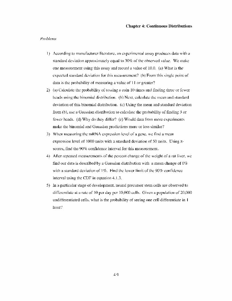
Problems

1) According to manufacturer literature, an experimental assay produces data with a

standard deviation approximately equal to 30% of the observed value. We make

one measurement using this assay and record a value of 10.0. (a) What is the

expected standard deviation for this measurement? (b) From this single point of

data is the probability of measuring a value of 11 or greater?

2) (a) Calculate the probability of tossing a coin 10 times and finding three or fewer

heads using the binomial distribution. (b) Next, calculate the mean and standard

deviation of this binomial distribution. (c) Using the mean and standard deviation

from (b), use a Gaussian distribution to calculate the probability of fmding 3 or

fewer heads. (d) Why do they differ? (e) Would data from more experiments

make the binomial and Gaussian predictions more or less similar?

3) When measuring the mRNA expression level of a gene, we find a mean

expression level of 1000 units with a standard deviation of 50 units. Using z-

scores, find the 90% confidence interval for this measurement.

4) After repeated measurements of the percent change of the weight of a rat liver, we

find our data is described by a Gaussian distribution with a mean change of 0%

with a standard deviation of 1%. Find the lower limit of the 90% confidence

interval using the CDF in equation 4.1.3.

5) In a particular stage of development, neural precursor stem cells are observed to

differentiate at a rate of 10 per day per 10,000 cells. Given a population of 20,000

undifferentiated cells, what is the probability of seeing one cell differentiate in 1

hour?

Chapter 5: Statistical Inference

5.0 Statistical Inference

In the previous sections we have introduced tools for statistical descriptions of

data, and shown how probability theory can be used to make some inference or prediction

based on data. In this chapter will introduce some commonly used statistical tools for

inference and show how they can be used in biological problems.

5.1 Confidence Intervals

When validating an experimental or computational result, we are often faced with

the question of how sure we are of a particular measurement or value. A statistical

method to evaluate this sureness is a confidence interval. A confidence interval simply

says that we are sure that the true value is somewhere within an interval with a given

probability (typically 95% or 99%). The concept of a confidence interval is illustrated in

the plot in Figure 5.1.0.

n95% coi~fidence interval n 9 9 % confidence intersal

Fi-me 5.1 .O: Illustration of a confidence interval around the mean value of a distribution.

Note that the shaded area encompasses the confidence interval region.


To find the range of values within a confidence interval, we integrate the

probability distribution function to find a symmetric region that covers the confidence

interval. Introductory statistics texts focus primarily on calculating confidence intervals

only for Gaussian distributions, however the same approach applies equally well for any

distribution of any shape, although the mathematics can be more challenging.

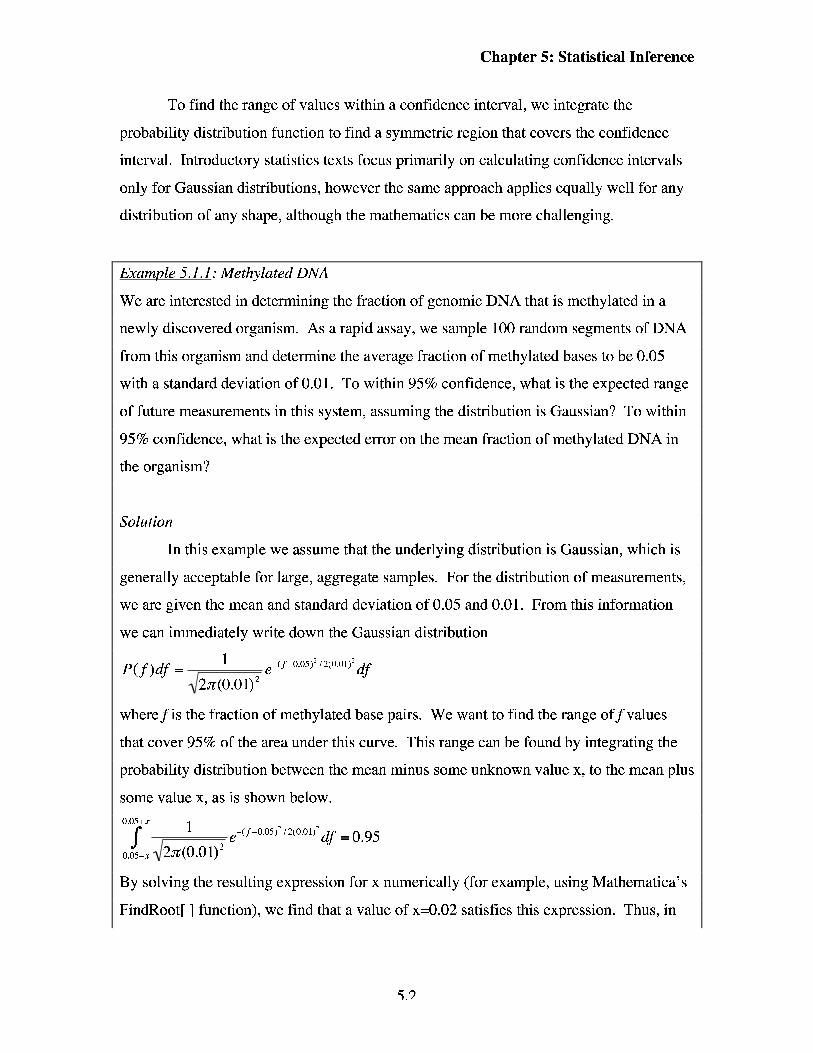
Example 5.1.1 : Methy luted DNA

We are interested in determining the fraction of genomic DNA that is methylated in a

newly discovered organism. As a rapid assay, we sample 100 random segments of DNA

from this organism and determine the average fraction of methylated bases to be 0.05

with a standard deviation of 0.01. To within 95% confidence, what is the expected range

of future measurements in this system, assuming the distribution is Gaussian? To within

95% confidence, what is the expected error on the mean fraction of methylated DNA in

the organism?

Solution

In this example we assume that the underlying distribution is Gaussian, which is

generally acceptable for large, aggregate samples. For the distribution of measurements,

we are given the mean and standard deviation of 0.05 and 0.01. From this information

we can immediately write down the Gaussian distribution

where f is the fraction of methylated base pairs. We want to find the range off values

that cover 95% of the area under this curve. This range can be found by integrating the

probability distribution between the mean minus some unknown value x, to the mean plus

some value x, as is shown below.

By solving the resulting expression for x numerically (for example, using Mathematica's

FindRoot[ ] function), we find that a value of x=0.02 satisfies this expression. Thus, in


future experiments we would expect 95% of our measurements to fall within the interval

0.05+0.02.

To find the expected error of the mean, we need to find the standard error of the

mean, as was introduced in chapter 1. To find this error we divide our given standard

deviation by the square root of the number of samples

Using this standard deviation of the mean as our standard deviation, we can now perform

the same calculation as before

Here we find that x=0.002 satisfies our equation. Thus we would expect that the true

mean for the whole genome lies somewhere within the range of 0.05&.002.

Example 5.1.2: Cell death

In response to radiation treatment of a particular cell line, 1 in 500 cells die each

minute. If we start with 2,500 cells, how many will likely die after one minute of

irradiation? To within a 90% confidence interval, what is the range of expected number

of cells to die after 1 minute of irradiation?

Solution

The data in this problem is given as a frequency of cell death per unit time, which

suggests that a Poisson distribution may be a good model for this system. We recall the

form of the Poisson distribution from Chapter 3

pke-" P,(k) = -

k !

where Y is the expected number of successes and k is the observed number of successes.

From the given data we find ~n, as

1 p=Np=2500-=5

500


Another common question in statistics is to ask what is the probability that a

specific assertion is right or wrong. To make such a clear result, we have to be careful in

specifying what we mean by right and wrong. We begin by deciding on a suitable null

hypothesis, commonly designated as &. A null hypothesis is a default case that

contradicts our hypothesis. For example, if we compare two means, our null hypothesis

may be that the means were actually drawn from the same distribution and the separation

Thus, we expect that on average 5 cells would die in response to this irradiation

procedure.

To calculate the error on this prediction, we need to find the boundaries that

encompass 90% of the probability density. This requirement can be expressed in the

following expression 5+x 5ke-5 - - 0.90

i= 5-x i= 5-x k!

This equation can be solved by trial and error with an x value of 3. Thus we are 90%

sure that after one minute of irradiation, between 2 and 8 cells will die from this

population. This range corresponds to the shaded area shown in Figure 5.2.2.

a17s 0.15 1 0.125 1

I ? 0.1

0.075

0.05

0.025

k

Fi-me 5.2.2: A Poisson distribution describing cell death for a population of 2,500 cells.

Shaded areas represent the 90% confidence region surrounding the mean at k=5.

:

-- , ,

:

n 0 1 2 3 4 5 A 7 K 9 1 0 1 1 12 13 1 4 1 5

-


is coincidental. Similarly, if we are searching for patterns in a DNA sequence, we might

use a random sequence as our null hypothesis. Our hypothesis is called the alternative

hypothesis, or HI. For the comparison of two means, the alternative hypothesis may be

that the two means are distinct.

Given this background, a p-value is defined as the probability that a set of

observations would assume a value greater than or equal to the observed value strictly by

chance. Thus, large p-values indicate that the result is likely to have happened by chance,

while low p-values indicate that random chance played less of a roll. In many

experimental contexts, p-values of less than 0.05 or 0.01 are considered statistically

significant, while larger values are too likely to have happened by random chance. This

cutoff is an arbitrary rule of thumb and may be too strict for some cases and not strict

enough for others, depending on the situation.

To calculate a p-value, we need to integrate the distribution generated by the

measurements, much like we did earlier to calculate confidence intervals. Examples of

how p-values would be calculated are shown in the following examples.

Example 5.2.1 : Geriatric Worms

The nematode C. elegans has a mean lifetime of 18 days with a standard deviation

of 10 days. After performing a silencing RNA (siRNA) screen to knockdown the

expression of combinations of genes, you find that worms exposed to a particular set of

siRNAs live on average 21 days. In total 37 worms were followed. Do these conditions

cause the nematodes to live longer? How significant is this finding?

Solution

To begin, we must choose which distribution to use to model our data. Because

the measurement is continuous (lifetime as measured in days), a continuous model is

most appropriate. As a first approximation we may also assume that the distribution is

symmetric and normally distributed, in which case we can write the distribution down

directly

J'(u0) = 1 e-(*-P)2 ,zo2

hno2


This distribution describes how the normal worm lifespan varies based on known data.

However, we are interested in seeing if the mean of this distribution is significantly lower

than 21 days, so we must use the standard error, or error of the mean to construct this

distribution

lo 1.64 op=x=J37=

Thus the distribution describing our alternative hypothesis is

1 -(x-18)' /2(1.64)' P(!40p) = d-e

To find the probability, or p-value, that the siRNA treatment results in longer

nematode life, we need to calculate the area under the probability distribution curve that

is 21 days or more, as is shown in the figure below. This area can be calculated directly

by integrating the distribution, which can be easily done for the Gaussian distribution as

was shown in the previous chapter (Eqn. 4.1.4) and is shown below

m

P(X r 21) = J P ( ~ O , ) ~ X = - ~ r f 21 1 ( [%I - Y[%])

=- 2 ' ( 1-Erf [1:1;;-])=0.034

Therefore the lifetime of the nematodes is longer than average, with a p-value of 0.034.

This p-value is less than the 0.05 criteria used by many researchers, and therefore may be

considered significant.


Example 5.2.2: Blood glucose levels

Blood glucose levels in humans have a mean of 170 mg/dL and a standard

deviation of 40 mg/dL. In a sample 100 of obese men and women, we find a mean

glucose level of 180 mg/dL. What is the probability that the obese population has a

normal glucose level?

Solution

In this case our null hypothesis is that the obese population has a mean blood

glucose level of 170 mg/dL, and the deviation that we saw from this value is a result of

random chance. The alternative hypothesis is that the obese population does not have a

mean glucose concentration of 170 mg/dL. These two assertions are summarized below

% p= 170 mg/dL

HI pz170 mg/dL

0.2

U.15

PI I A ~ ~ J ~ ~ I 0.1

0.05

. r\ / \ i

. / ", i '\

i - i \

i ', . / ",

\

. . . . . . . . . . . 13 15 17 19 2 1 2 3 28

lifetime (days)

Fi-me 5.2.1: A graphical example of a p-value calculation. In this case, the p-value

represents the probability that the lifetime of the worms is 21 days or more by chance.

This value is proportional to the shaded area on the right of the figure.

Note that this example is what is called a one-tailed test, meaning that only one

side of the distribution was integrated. We only integrate one side because we are only

interested in the probability that our observed data means that worms live longer.


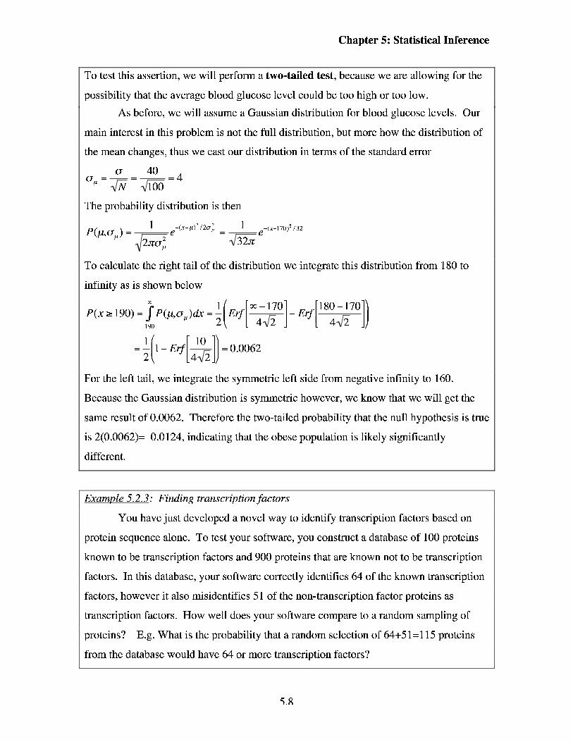
To test this assertion, we will perform a two-tailed test, because we are allowing for the

possibility that the average blood glucose level could be too high or too low.

As before, we will assume a Gaussian distribution for blood glucose levels. Our

main interest in this problem is not the full distribution, but more how the distribution of

the mean changes, thus we cast our distribution in terms of the standard error

o 40 O ; = X = = = ~

The probability distribution is then

- -(x-170)' 132 --

To calculate the right tail of the distribution we integrate this distribution from 180 to

infinity as is shown below CO

a - 170 P(x 2 190) = $ P ( ~ o ~ ) ~ x = - Eif

190 2

2

For the left tail, we integrate the symmetric left side from negative infinity to 160.

Because the Gaussian distribution is symmetric however, we know that we will get the

same result of 0.0062. Therefore the two-tailed probability that the null hypothesis is true

is 2(0.0062)= 0.0124, indicating that the obese population is likely significantly

different.

Example 5.2.3: Finding transcription factors

You have just developed a novel way to identify transcription factors based on

protein sequence alone. To test your software, you construct a database of 100 proteins

known to be transcription factors and 900 proteins that are known not to be transcription

factors. In this database, your software correctly identifies 64 of the known transcription

factors, however it also misidentifies 51 of the non-transcription factor proteins as

transcription factors. How well does your software compare to a random sampling of

proteins? E.g. What is the probability that a random selection of 64+51=115 proteins

from the database would have 64 or more transcription factors?


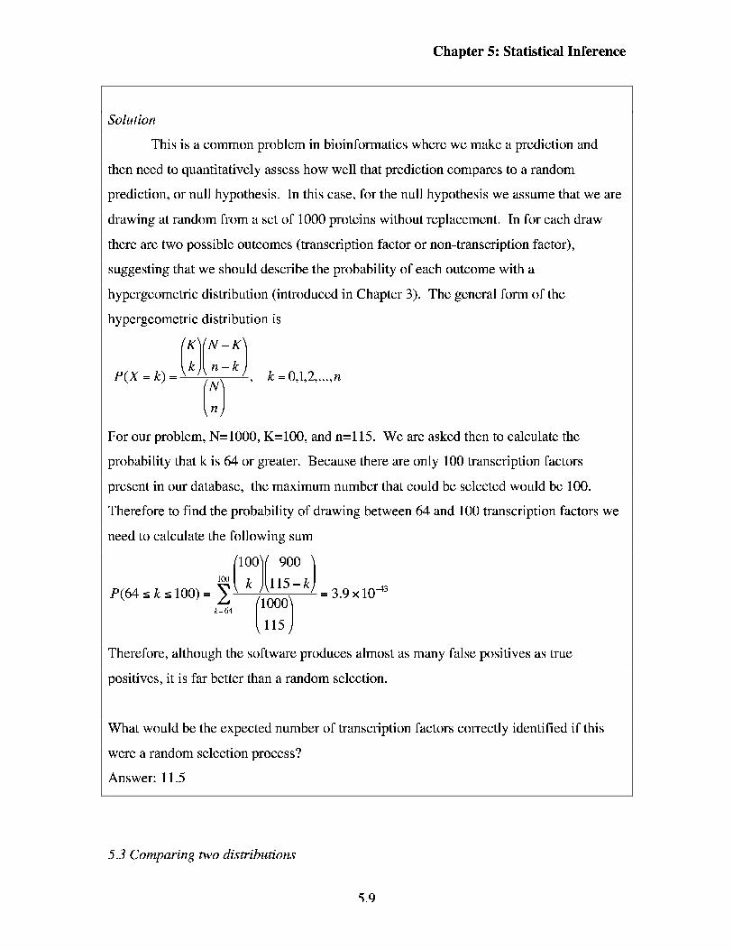
Solution

This is a common problem in bioinformatics where we make a prediction and

then need to quantitatively assess how well that prediction compares to a random

prediction, or null hypothesis. In this case, for the null hypothesis we assume that we are

drawing at random from a set of 1000 proteins without replacement. In for each draw

there are two possible outcomes (transcription factor or non-transcription factor),

suggesting that we should describe the probability of each outcome with a

hypergeometric distribution (introduced in Chapter 3). The general form of the

hypergeometric distribution is

P(X = k) = (:I(: 1 f) , k =0,1,2 ,..., n

(3 For our problem, N=1000, K=100, and n=115. We are asked then to calculate the

probability that k is 64 or greater. Because there are only 100 transcription factors

present in our database, the maximum number that could be selected would be 100.

Therefore to find the probability of drawing between 64 and 100 transcription factors we

need to calculate the following sum

100

P(64 s k s 100) = 2 (?)(I I!? k) = 3.9 loA3

.=@ (:-:I Therefore, although the software produces almost as many false positives as true

positives, it is far better than a random selection.

What would be the expected number of transcription factors correctly identified if this

were a random selection process?

Answer: 11.5

5.3 Comparing two distributions


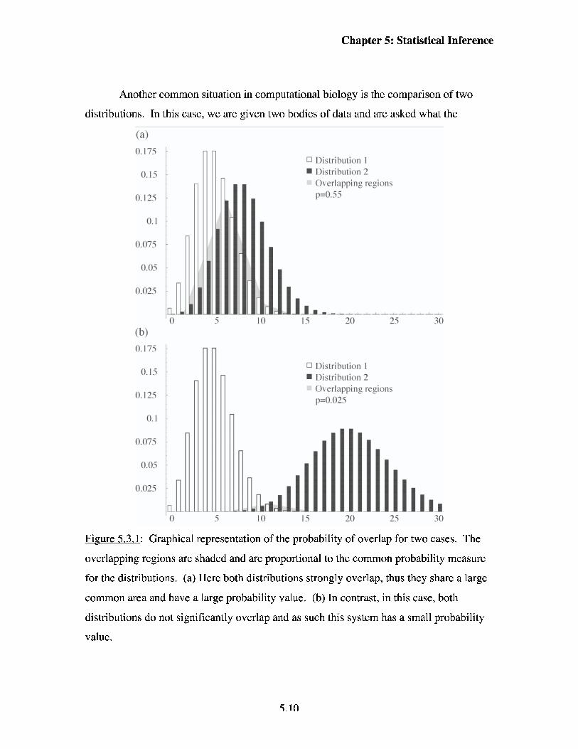
Another common situation in computational biology is the comparison of two

distributions. In this case, we are given two bodies of data and are asked what the

(a)

nislribulioli 1 nislribulioli 2 Overlapping regions p-0.55

Distribution 1 Distribution 2 Overlapping regions p=I_).U25

5 1 0 15 20 25 3 1)

Fi-me 5.3.1: Graphical representation of the probability of overlap for two cases. The

overlapping regions are shaded and are proportional to the common probability measure

for the distributions. (a) Here both distributions strongly overlap, thus they share a large

common area and have a large probability value. (b) In contrast, in this case, both

distributions do not significantly overlap and as such this system has a small probability

value.


probability is that both of these sets of data were drawn from the same distribution. This

probability is similar to the p-value described in section 5.2, but is more general.

Graphically, the probability that two distributions are the same is the overlapping region

of two probability distributions, as is shown in Figure 5.3.1.

In general to calculate a probability value from two distributions, we need to

integrate or sum the area encompassed by both distributions. This can be stated explicitly

using a piece wise function as

P(overlap) = s rnin -m

where p, and p, are two continuous probability distributions, and 8, and 8, are the

parameters for those distributions. Similarly for two discrete distributions

Essentially, we are making an explicit measure of what area these two distributions have

in common, as is illustrated in the Venn diagrams in Figure 5.1.2 below.

Fi-me 5.3.2: Venn diagram schematic of how probability values can be calculated for

arbitrary distributions. Note that the greater the overlapping area, the larger the

probability value.

Example 5.3.1: Protein expression

Imagine that we are running an experiment to see if the presence of a drug causes

the up regulation of a particular enzyme within the p450 family. We make 30

measurements of the protein expression level in the absence and presence of the drug, for

a total of 60 experiments. From these experiments, we find that the protein expression

level with the drug has a mean value of 615 units with a standard deviation of 45 units.

In the absence of the drug, the expression level is 575 units with a standard deviation of

60 units. What is the probability that the drug causes the enzyme to up regulate?


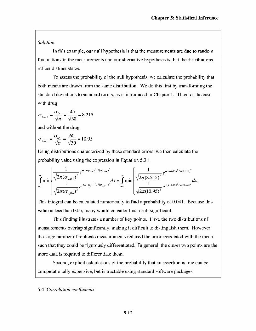
Solution

In this example, our null hypothesis is that the measurements are due to random

fluctuations in the measurements and our alternative hypothesis is that the distributions

reflect distinct states.

To assess the probability of the null hypothesis, we calculate the probability that

both means are drawn from the same distribution. We do this first by transforming the

standard deviations to standard errors, as is introduced in Chapter 1. Thus for the case

with drug

45 GPO+ = aD'= - - & 1/30

- 8.215

and without the drug

60 op,- = %= = - = 10.95 & 1/30

Using distributions characterized by these standard errors, we then calculate the

probability value using the expression in Equation 5.3.1

1 -(x-PD+ )' 12(oU,p+ 1' 1 -(x-615)' 12(8.215)'

I j ~ n p 3 e 1 d i = j+ - min d m e 1 dx

-m )' 12(uu,P- )' -CO -(x-575)' 12(10.95)'

~~e .\/we This integral can be calculated numerically to find a probability of 0.041. Because this

value is less than 0.05, many would consider this result significant.

This finding illustrates a number of key points. First, the two distributions of

measurements overlap significantly, making it difficult to distinguish them. However,

the large number of replicate measurements reduced the error associated with the mean

such that they could be rigorously differentiated. In general, the closer two points are the

more data is required to differentiate them.

Second, explicit calculations of the probability that an assertion is true can be

computationally expensive, but is tractable using standard software packages.

5.4 Correlation coeficients


Sometimes we encounter situations where we are given two sets of data that seem

to scale with each other, but not perfectly. In this case, we can assess how well these two

variables correlate with each other by using the correlation coefficient, or as it is

sometimes called Pearson's correlation. Most of us have encountered the correlation

coefficient as the ? fit of data to a line. Values of the correlation coefficient that are near

one indicate a strong correlation, while values near zero indicate a poor correlation.

The correlation coefficient is defined as

where ss,,, ss,,, and ss, are defined as

ss, - C ( x - X)2

Here, bars over variables indicate an average value. Thus s%, is the sum of the squared

deviation of x from its mean.

Example 5.4.1: Gene clustering

A widely used approach in analyzing expression array data is to cluster genes that

behave similarly under a wide variety of physiological conditions. One method to

quantify how well two genes track each other is to calculate their correlation coefficient.

Thus, imagine that we have gathered the following rnRNA expression data for two genes

over ten different conditions. The raw data for from these experiments are listed below:

Experiment # expression index of gene 1 expression index of gene2 1 645 9045 2 1284 16943 3 523 6534 4 3045 33928 5 203 3698 6 1009 11960 7 1132 14850 8 1894 20394 9 834 20394 10 2300 25290


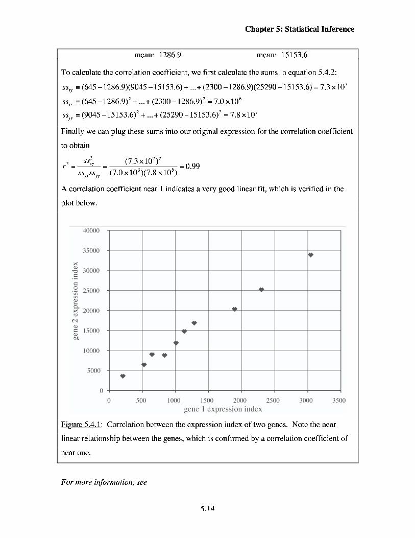
mean: 1286.9 mean: 15153.6

To calculate the correlation coefficient, we first calculate the sums in equation 5.4.2:

SS, = (645 - 1286.9)(9045 - 15153.6) + ... + (2300 - 1286.9)(25290 - 15153.6) = 7.3 x lo7

SS, = (645 - 1286.9)~ + ... + (2300 - 1286.9)~ = 7.0 x lo6

ssp = (9045 - 15153.6)' + ...+ (25290 -15153.6)' = 7.8 x 10'

Finally we can plug these sums into our original expression for the correlation coefficient

to obtain

2 y =-- - (7.3 x 10712 = 0.99

ss,ss, (7.0 x 106)(7.8 x lo8)

A correlation coefficient near 1 indicates a very good linear fit, which is verified in the

plot below.

4001KI

35UIX)

K s ::0000 E . - r

25000 rh

2 2 200m @d

Pl

151XXI WJ

1 OOlKI

SII011

0

0 5 00 I 000 1500 2000 2500 3000 3500 gene 1 exyressiol~ index

Fi-me 5.4.1: Correlation between the expression index of two genes. Note the near

linear relationship between the genes, which is confirmed by a correlation coefficient of

near one.



Chapter 7 of "The Cartoon Guide to Statistics" by L. Gonick and W. Smith

Eric Weissteins's World of Mathematics at mathworld.wolfram.com



Chapter 6 in "Elementary Statistics" by M. F. Triola


Problems

1) If we toss a fair coin four times, we expect to see two heads and two tails. If we

allow that we might see 1,2, or 3 heads, then what confidence interval are we

covering? Said another way, what percent of the time will we see between 1 and

3 heads?

2) The average migration speed of an isolated neutrophil is 20 pmlmin. After

treatment with an ERK inhibitor, we observe 25 neutrophils and find an average

migration speed on 18 prrdmin with a standard deviation of 6 prrdmin. Is this

speed significantly slower than average for neutrophils? What is the p-value?

3) Imagine a simple saw-tooth type distribution defined by

(a) Plot this distribution.

(b) Show that the total area under this distribution exactly equals one.

(c) Find the expectation value or mean of this distribution (show your work).

(d) Calculate the range around the mean that encompasses a 99% confidence

region.

4) (a) Plot by hand the following two distributions:

P,(x) = 2x

P,(x) = 2(1- x)

where x is defined from zero to one. (b) What is the probability that these two

distributions were drawn from the same original distribution? Hint: find the area

of the overlapping area.

5) The histograms in Figure 5.3.1 were calculated from Poisson distributions. In

panel (a), the expected number of events are p1=5 and ~ = 8 . Show how you

would find the probability that these two distributions are significantly different.

Do we really need to sum from 0 to infinity, or can we stop at a smaller value of

k? Why or why not? Hint: Set up the problem as shown for a discrete

distribution in Equation 5.3.2.

Appendix A: Dirichlet Distribution

A.1 Dirichlet Distribution

The Dirichlet distribution is a continuous distribution that can be employed with

systems that have many outcomes. One way to think of the Dirichlet distribution is as a

continuous counterpart of the multinomial distribution. The Dirichlet distribution is

commonly employed as a prior distribution in Bayesian statistics as it yields analytically

tractable expressions for an arbitrary number of variables.

The Dirichlet distribution for K possible outcomes has the following form

where r is the gamma function, which is a continuous version of the factorial function.

For any real positive number x, the gamma function is defined as

r ( x + 1) = x ~ ( x ) (A. 1.2)

The constants ai in Eqn. A. 1.1 specify the particular shape of the distribution and must be

real valued and positive. The parameter €Ii is the probability of outcome i. As is the case

for probabilities they must be between 0 and 1 and their sum total must equal 1.

For the Dirichlet distribution, the mean is described by the normalized

parameters. For example, the mean value of €Ii is

(A. 1.3)

Also, the tightness of the distribution is defined by the value of a, with larger values

leading to sharper distributions.

In the limiting case of K=2, these distributions reduce down to a subclass of

distributions known as the beta distribution which closely resembles the binomial

distribution and is shown below

(A. 1.4)


A central difference between the beta distribution and the binomial distribution is not

their functional forms, but is more how they are used. The binomial distribution is most

often used to describe the probability of various configurations of outputs, while the beta

distribution is used to describe the probability of the probability parameters, 0. Plots of

the beta distribution for various values of a, and a, are shown in Figure A. 1.1.

81 @ I

Fi-me A. 1.1: Plots of the beta distribution for various values of a, and a,. Note that

equal a values produce a symmetric distribution, while unequal values a produce an

asymmetric distribution. In addition, larger a values produce a tighter distribution.

Example A.1 .I : Liquid handling robots

We are assessing two high-throughput liquid handling robots. To test the robots

we have them dilute a fluorescently labeled solution to 50% of its original concentration.

Both robots produce solutions that have an average of 50% less fluorescence with errors

described by a beta distribution, but for robot A a,= %=lo, while for robot B, a1=a,=15.

The cost per experiment with robot A is $2.25 while the cost per experiment with robot B


is $3.00. If we assume a measurement error of more than *5% means that the experiment

must be repeated, then which robot is more economical?

Solution

Here we replace our probability measurement, 0,, with the measured fraction of

fluorescence in the resulting solution. This measure has the same properties as a

probability in that it cannot be negative and all fractions must sum to one, so this is a

valid replacement. First, we write out the Beta distribution for this system

r(a1+ a 2 ) Qa, -'(I - el)..-' r(a1 ) For robot A we have the distribution

r(20) ,$O-l(l- ~~)lo-l r(io)r(io) For robot B we have

r(30) e;5-1(1- el)"' r(15)r(15)

We would predict that given the higher alpha values of robot B, that robot B would

produce more reliable data. We quantify this prediction by integrating these expressions

over the fraction, 0,, from 0.45 to 0.55 to determine what fraction of the experiments

would be passable. For robot A we find

- 0.55 r(20) PA - J r(io)r(io) e;O-l (1 - el)lO-l do1 = 0.342 0.45

For robot B we find

- 0.55 ~ ( 3 0 ) pB gYYd - Jr(is)r(is) 6:"-'(l- %,)15-1d01 = 0.414

0.45

To find which robot is more economical, we calculate the average cost of getting at least

one passable result. All good results will require at least one experiment, so the initial

cost is fixed. A second experiment will only need to be run if the first experiment does

not work. Similarly a third experiment will be needed if the second does not work, and

on and on. This cost can be represented by a weighted sum of probabilities


m

. CO (cost) = 1 cop; = - i= o 1- pf

where Co is the cost of each experiment and p, is the probability of failure. The brackets

surrounding cost denote the expected cost. Performing this calculation for both machines

we find

(cost*) = $6a5Xeasurement

(cost,) = $7*2Xeasurement

Therefore, although machine B produces more accurate data, its additional cost is not

justified.

A primary use of the Dirichlet distribution is in solving problems in Bayesian

statistics. The reason for this is that Bayesian statistics requires that we state our

uncertainty about a parameter value, for example, in the form of a probability

distribution. Dirichlet distributions have the advantage that they can describe phenomena

with an arbitrary number of outcomes and are relatively easy to integrate with

multinomial distributions used in probability calculations. An example of how these

distributions work together is shown in Example A. 1.2.

Example A.1.2: Hair pheno~pes

Imagine that we are interested in the mechanisms that govern hair phenotypes.

Literature data has shown that mutations in a key gene responsible for hair development

result in three distinct phenotypes: thick hair, thin hair, and no hair. However, no

available data indicates the relative frequency of these three phenotypes, so we run our

own experiment in mice. Our first litter yields four mice with the thick hair phenotype,

and one with the thin hair phenotype and none with the no hair phenotype. Given this

information, what is the expected fraction of mice with each phenotype?

Solution

This problem represents a common situation in biological research, as we have

some background data plus a small body of experimental data. However, this situation


presents a problem for traditional frequentist statistics, due to the small dataset size. For

example, in this dataset, we do not see any mice with the no hair phenotype, although we

know that they exist. It would be imprudent to assign a zero probability to this phenotype

based on such a small sample size, but what other options do we have?

This conflict can be addressed using Bayesian statistics, multinomial

distributions, and Dirichlet distributions. To begin, we introduce a number of variables to

describe the problem. The unknown probability of each phenotype can be written as el ,

02, and 8,. The sum of these probabilities must equal one by definition. Similarly, the

counts for each phenotype can be written as n,, n,, and n3. The probability of these

counts can then be expressed as the following multinomial distribution

(n, + n2 + n3)! p(nl,n2,n3 1ol,02>03) =

nl!n2!n3!

However, our goal is not to find the probability of our data, but instead to find the

probability of our probability parameters given our data. This rearrangement can be

found using Bayes' rule as is shown below

This expression can be simplified by dropping the denominator on the right hand side, as

the probability of the data alone does not depend on the parameters and as such is a

constant (we will come back to this at the end of the problem). Thus the probability that

we are interested in reduces to

p(ol,02,03 nl,n29n3) cc p(nl,n,,n3 I ol,02~03)p(ol,02,03)

The first term in this expression is the multinomial distribution generated above. The

second term is our prior belief about the parameters. This term can be simply defined as

a Dirichlet distribution of the following form

One of the most frequent uses of Dirichlet distribution is in defining a prior for a

Bayesian calculation involving multinomial distributions. To completely define this

distribution, we have to choose values for the hyper parameters, a,, a,, and a,. Because

we have no particular information in this case, we can assign what is known as a uniform


3rior, meaning that any value of 0 is equally likely. This uniform prior is assigned by

setting a,= %= a,=l, which generates a flat line as is shown in Figure A. 1. la. By

substituting in these a values and merging both expressions we generate the following

:xpression for the posterior probability of our parameters given data

(% + n2 + p(el,e2,e3 I %,n2,n3) nl!n2! n,!

which simplifies to

W s final form is essentially a Dirichlet distribution also. When we enter our

:xperimental data we obtain the following expression

W s expression describes a probability density function that represents our certainty

ibout each of the probabilitie parameters, el, O,, and 8,. Noting that the last probability is

aised to the zero power, we can express this density in terms of only two variables

4 density plot of this function is shown in Figure 4.2.2.

increasing ~robabil density

posterior expectation value *

prior expectation value *


Figure 4.2.2: Plot of the posterior probability density given in Example A.2.2. Note that

the probability density increases for both parameters as they approach one, however the

posterior expectation value is not at the point of highest probability.

To find the expectation values for el , 8,, we integrate over all possible values of

each variable

I 5!r(3) I 5(e2)

) = SO01 4!1!0!r(1)~(1)~(1) 0, 0,dOl = -

3

5!r(3) lo(e,)' (02) = S:02 4!1!0!r(1)r(1)r(1) = 3

I 5!r(3)

(03) = e3 4!1!0!r(1)~(1)~(1) e;e;de3 = ~ ( 0 , ) ~ (0,)

Solving for each of these values we obtain

(4) = 0.564

(0,) = 0.338

(e3) = 0.172

We are almost there. If we sum these values we note that they equal 1.074, not 1.00 as

we require them. This is because we ignored the normalizing term in our original

probability statement, p(nl,n2,n3). We can now correct for this omission by dividing all

values by this normalizing constant 1.074 to obtain

(el)'= 0.525

(0,)' = 0.3 15

(e,)' = 0.160

Therefore from this small sample size of 5 observations, we are able to rigorously

define the probability of various outcomes while accurately representing our uncertainty.


Eric Weissteins's World of Mathematics at mathworld.wolfram.com




David Heckeman's "A Tutorial on Learning with Bayesian Networks" in

Learning in Graphical Models, edited by Michael I Jordan.

"Data Analysis: A Byesian Tutorial" by D. S. Silva

"Bayesian Inference in Statistical Analysis" by G. E. Box and G. C. Tiao.


Problems

1) We observe that a protein has two distinct phosphorylation sites, A and B. We

run a single experiment and find that only site A is phosphorylated, while B is

not. Based on this single experiment, what can we say about the probability of

finding A and B each phosphorylation configuration (e.g. AB, Q,, b B , and

AB,, where the p subscript indicates that the site is phosphorylated)? How well

would you expect a probabilistic model to describe this system? Why?

Hint: this problem is much like example A. 1.2.

Appendix B: Bayesian Networks

B.1 Bayesian Networks

Thus far we have introduced tools from probability theory to describe events that

are independent and dependent. Although we have only dealt with examples that contain

a small number of variables, the theory applies equally well to describe systems with an

arbitrary number of variables. For example, a probabilistic model could be used to

describe interactions between genes based on expression data containing thousands of

variables.

However, when constructing a probability model with many variables, we

encounter a number of problems. As an illustration, imagine that we have collected

absentlpresent data for the expression level of 10 different genes over a variety of

physiological conditions. Let us call each expression level a variable xl,x2,. . .,xlo. Based

on this information, we can then predict the value of any one variable assuming the

values of the other 9 are known e.g.

P(x1 1 ~29....9~1,,) (B.1.1.)

However, to construct this probability distribution will take a large number of

experiments for there are 29 (=512) different possible states that x2-xlo could take on.

Similarly, we might suspect that the expression level of some genes is more predictive of

the expression level x,, but this analysis does not tell us which relationships are more or

less important.

These problems suggest that we might be able to break the probability

distribution into independent and dependent parts. For example, we might know that the

expression level of gene 2 is independent of the expression level of gene 1. With this

information we can then rewrite the probability of finding gene one in any state as:

p(xl x'39****9x10) (B.1.2)

Conceivably, we could have many interactions that are independent of one another, so for

each of these we could construct a simplified conditional probability statement. As we

simplify the conditional probability statement, we then need less data. For example, in

removing the dependence on gene 1 from equation B. 1.1 to B. 1.2 we reduced the total

number of parent states (conditioning states) from 29 to 28 , a change of 256 states.


A convenient way to organize and represent these groups of conditional

probability relationships is as a Bayesian network. A Bayesian network is a directed

acyclic graph representation of a joint probability statement. Taking the gene expression

model introduced above, we could make many simplifications to the network to generate

the following probability statement

P(xl?x2?.*.*?x,,) = I x2?x3)P(x2 I x4?x,?x,)P(x3 I x2)P(x4)

P(x,)P(x, I x,?x,,x,)P(x, I x,o)p(x,)p(x,)p(x,o)1

We can represent this as a Bayesian network by drawing each variable as a node, with

arrows connecting variables that are conditionally dependent on each other. A graph of

the statement in equation B. 1.3 is shown in Figure B. 1.1

Figure B .1.3 : A Bayesian network representation of the conditional dependency

statements in equation B. 1.3.

If we do not already know the graph structure of a Bayesian network, then it is

also possible to derive this connectivity from data alone. In this way, we can rapidly

identify strong relationships between variables that may not have been apparent using

other tools for data analysis. For example, the status of a single gene could be dependent

on the states of three other genes in a complex but reproducible way. Such relationships

become immediately apparent from the Bayesian network structure, as shown in Figure

B.1.3.

A classic example of a Bayesian network is a family tree that would be used in

genetics or genetic counseling. In this tree, each person is a node and arrows connect

parents to children. From the conditional probability standpoint, this graph structure

makes sense, for if we are trying to predict the probability that a grandchild carries a

genetic particular mutation, we know that the most direct predictor is the genetic state of


the parents. Assuming no inbreeding, the genetic states of the mother and father should

be independent, so there is no arrow directly connecting these two people.


David Heckeman's "A Tutorial on Learning with Bayesian Networks" in

Learning in Graphical Models, edited by Michael I Jordan (1998).

"Bayesian Inference in Statistical Analysis" by G. E. Box and G. C. Tiao (1992).

"An introduction to Bayesian networks" by Finn V. Jensen (1996)


Problems

1 . Convert the following statements of conditional probabilities into a Bayesian

network graph.

a. P ( A I B)P(B I C,D, E)P(C I D)P(E I F)P(F)P(D)

b. P(AIB,C)P(BID)P(CID)P(D)

c. P ( A I B,C)P(B I C)P(C)P(D I E)P(E)

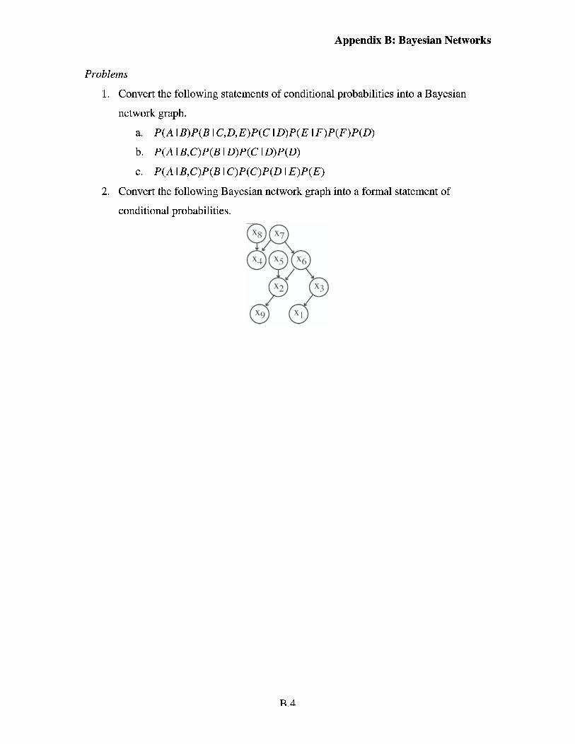
2. Convert the following Bayesian network graph into a formal statement of

conditional probabilities.

Appendix C: Solutions

Here we list the solutions to some of the exercises at the end of each chapter.

Note that in some cases we provide only the numerical answer, as this section is meant as

a self-check.

Chapter I : Common Statistical Terms

1) mean=2.223, standard deviationS.955

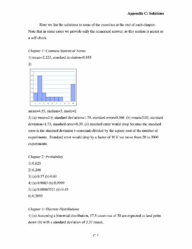
2)

mean=4.55, median=3, mode=2

3) (a) mean=2.9, standard deviation=1.79, standard erro-0.566 (b) mean=3.05, standard

deviation=1.73, standard erro~0.39. (c) standard error would drop because the standard

error is the standard deviation (-constant) divided by the square root of the number of

experiments. Standard error would drop by a factor of 10 if we move from 20 to 2000

experiments.

Chapter 2: Probability

1) 0.625

2) 0.248

3) (a) 0.37 (b) 0.61

4) (a) 0.9083 (b) 0.9999

5) (a) 0.00083521 (b) 0.45

6) 0.2092

Chapter 3: Discrete Distributions

1) (a) Assuming a binomial distribution, 17.5 tosses out of 50 are expected to land point

down (b) with a standard deviation of 3.37 tosses.


2) (a) Geometric distribution, p=0.236839 (b) Hypergeometric distribution for 1 to10

GPCRs, p= 0.23687 1. (Note this second calculation is non-trivial.)

3) Assuming a Poisson distribution,(a) p(O)= 0.00673795, (b) p(10)= 0.0181328.

4) Using a multinomial distribution, p=0.005467.


1) (a) Following the manufacturer literature, the standard deviation for the measurement

should be (10)(0.30)=3.

(b) Given normally distributed errors around a mean of 10 with a standard deviation of 3,

we can use the CDF in equation 4.1.3 to calculate the probability of making a

measurement of between negative infinity and 1 1 :

Therefore the probability of measuring a value of 11 or greater is just one minus the

above value, or 0.3694.

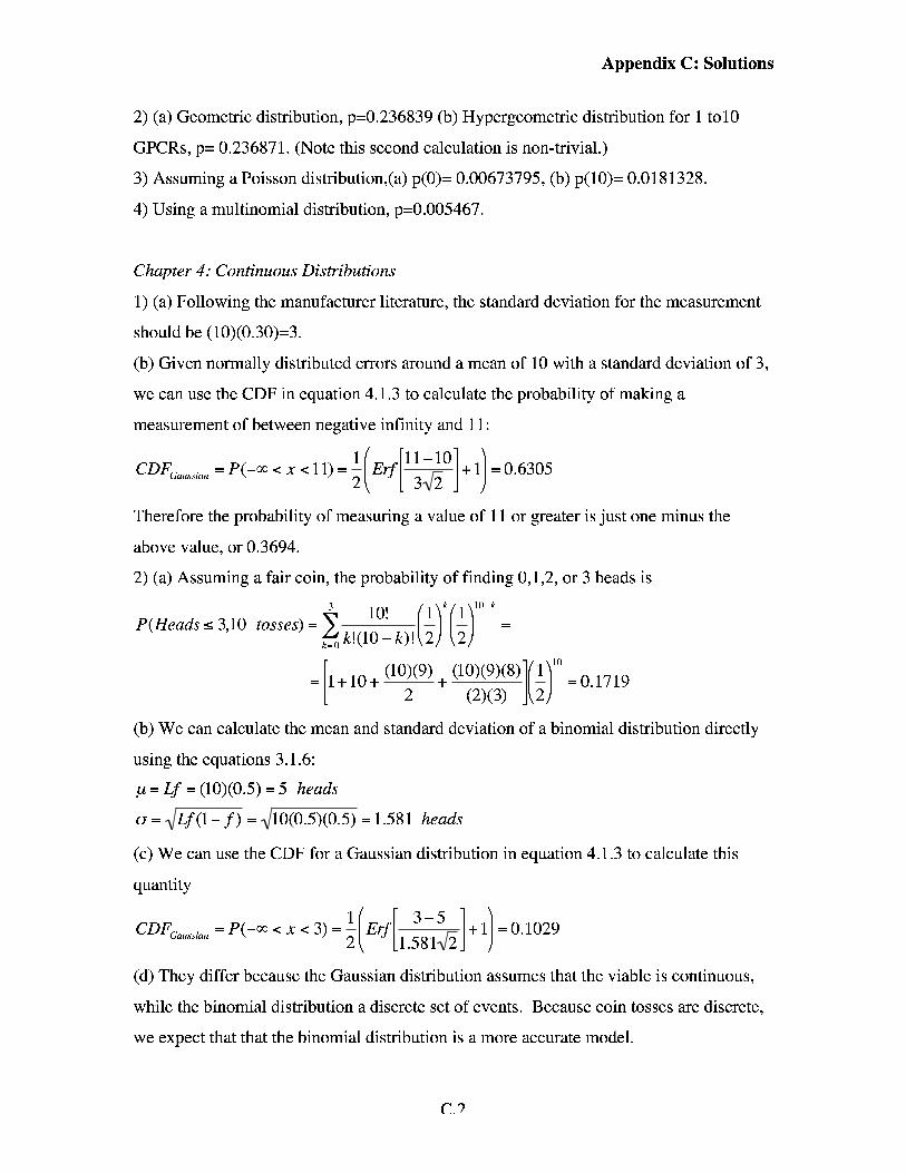
2) (a) Assuming a fair coin, the probability of finding 0,1,2, or 3 heads is

3

P(Heads s 3,10 tosses) = 1 - - k= 0

(b) We can calculate the mean and standard deviation of a binomial distribution directly

using the equations 3.1.6:

p= Lf = (10)(0.5) = 5 heads

a = d m = d w = 1 . 5 8 1 heads

(c) We can use the CDF for a Gaussian distribution in equation 4.1.3 to calculate this

quantity

(d) They differ because the Gaussian distribution assumes that the viable is continuous,

while the binomial distribution a discrete set of events. Because coin tosses are discrete,

we expect that that the binomial distribution is a more accurate model.


(e) More experiments should reduce the difference between the Gaussian and binomial

predictions. In the limit of an infinite number of experiments, the Gaussian and binomial

distributions should converge.

3) For the 90% confidence interval, we use a z-score of 1.645, mean of 1000, and

standard deviation of 50. Plugging into equation 4.2.1 and solving for x we obtain an

upper limit of 1082.25. A lower limit is found by using a z-score of -1.645, yielding an

x of 917.75. The 90% confidence interval is therefore 917.75 to 1082.25 units.

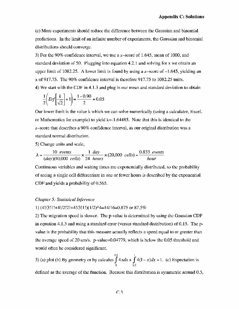
4) We start with the CDF in 4.1.3 and plug in our mean and standard deviation to obtain

Our lower limit is the value k which we can solve numerically (using a calculator, Excel,

or Mathematics for example) to yield k=-1.64485. Note that this is identical to the

z-score that describes a 90% confidence interval, as our original distribution was a

standard normal distribution.

5) Change units and scale,

10 events day x (20,000 cells) =

0.833 events A= X (day)(10,000 cells) 24 hours hour

Continuous variables and waiting times are exponentially distributed, so the probability

of seeing a single cell differentiate in one or fewer hours is described by the exponential

CDF and yields a probability of 0.565.


1) (4!/3! 1 !+4!/2!2!+4!/3! 1 !)(1/2)A4=14/16=0.875 or 87.5%

2) The migration speed is slower. The p-value is determined by using the Gaussian CDF

in equation 4.1.3 and using a standard error (versus standard distribution) of 0.15. The p-

value is the probability that this measure actually reflects a speed equal to or greater than

the average speed of 20 u d s . p-value=0.04779, which is below the 0.05 threshold and

would often be considered significant. 0.5 I

3) (a) plot (b) By geometry or by calculus $4xdx + $4(1- x)dx = 1. (c) Expectation is 0 0.5

defined as the average of the function. Because this distribution is symmetric around 0.5,


the expectation is 0.5. This can also be shown by calculus: 0.5 1

$(x)4xdx + $(n)4(1- x)dx = 0.5 (d) Again, because the distribution is symmetric, we 0 0.5

can do this calculation for half of the distribution. This could be done with calculus, or

just algebra. Using algebra, we know that the total area under the left half of the

distribution is (height*width)/2=((4*0.5)*0.5)/2=0.5. At the 99% confidence interval, we

would leave an area on the left hand side of (1.0-0.99)*(0.5)=0.005. A similar triangle

with an area of 0.005 can be described as (height*width)/2=area thus (4x*x)/2S.005,

thus x=0.05 at the lower bound of the 99% confidence interval. The upper bound is

x=1 .O-0.05S.95.

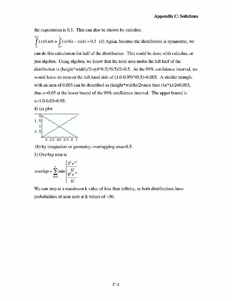
4) (a) plot

(b) by integration or geometry, overlapping area=05.

5) Overlap area is

We can stop at a maximum k value of less than infinity, as both distributions have

probabilities of near zero at k values of -50.

Documents

Chapter 4: Continuous Distributions 4.0 Continuous ...dspace.mit.edu/bitstream/handle/1721.1/66488/7-89-fall-2007/... · continuous and discrete distributions is that summing in discrete