Chapter 38Quantum Mechanics

• Quantum Mechanics – A New Theory

• The Wave Function and Its Interpretation; the Double-Slit Experiment

• The Heisenberg Uncertainty Principle

• Philosophic Implications; Probability versus Determinism

• The Schrödinger Equation in One Dimension –Time-Independent Form

• Time-Dependent Schrödinger Equation

Units of Chapter 38

• Free Particles; Plane Waves and Wave Packets

• Particle in an Infinitely Deep Square Well Potential (a Rigid Box)

• Finite Potential Well

• Tunneling Through a Barrier

Units of Chapter 38

Quantum mechanics incorporates wave-particle duality, and successfully explains energy states in complex atoms and molecules, the relative brightness of spectral lines, and many other phenomena.

It is widely accepted as being the fundamental theory underlying all physical processes.

Quantum mechanics is essential to understanding atoms and molecules, but can also have effects on larger scales.

38.1 Quantum Mechanics – A New Theory

An electromagnetic wave has oscillating electric and magnetic fields. What is oscillating in a matter wave?

This role is played by the wave function, Ψ. The square of the wave function at any point is proportional to the number of electrons expected to be found there.

For a single electron, the wave function is the probability of finding the electron at that point.

38.2 The Wave Function and Its Interpretation; the Double-Slit

Experiment

For example: the interference pattern is observed after many electrons have gone through the slits. If we send the electrons through one at a time, we cannot predict the path any single electron will take, but we can predict the overall distribution.

38.2 The Wave Function and Its Interpretation; the Double-Slit

Experiment

Quantum mechanics tells us there are limits to measurement – not because of the limits of our instruments, but inherently.

This is due to wave-particle duality, and to interaction between the observing equipment and the object being observed.

38.3 The Heisenberg Uncertainty Principle

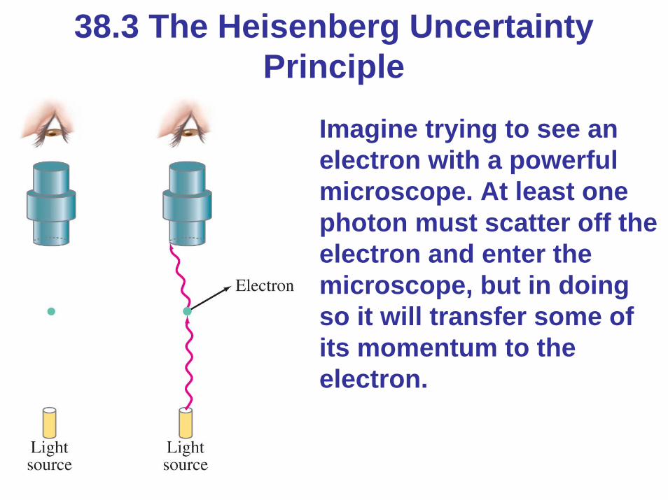
Imagine trying to see an electron with a powerful microscope. At least one photon must scatter off the electron and enter the microscope, but in doing so it will transfer some of its momentum to the electron.

38.3 The Heisenberg Uncertainty Principle

The uncertainty in the momentum of the electron is taken to be the momentum of the photon – it could transfer anywhere from none to all of its momentum.

In addition, the position can only be measured to about one wavelength of the photon.

38.3 The Heisenberg Uncertainty Principle

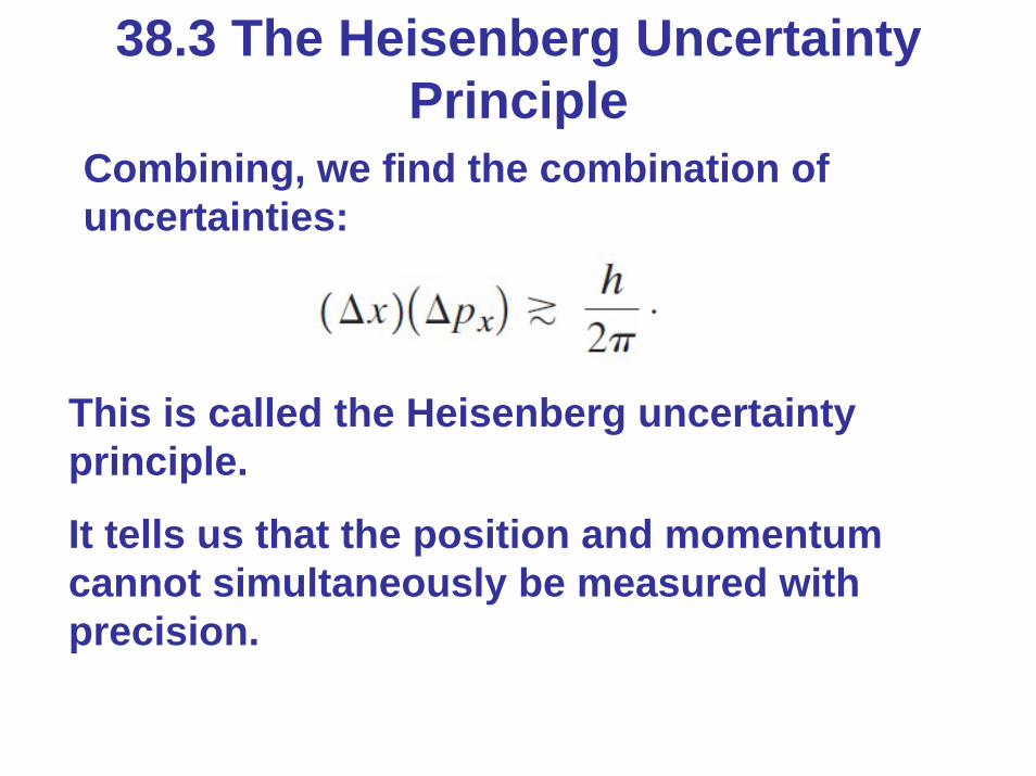
Combining, we find the combination of uncertainties:

This is called the Heisenberg uncertainty principle.

It tells us that the position and momentum cannot simultaneously be measured with precision.

38.3 The Heisenberg Uncertainty Principle

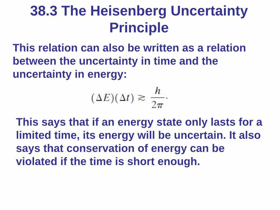
This relation can also be written as a relation between the uncertainty in time and the uncertainty in energy:

This says that if an energy state only lasts for a limited time, its energy will be uncertain. It also says that conservation of energy can be violated if the time is short enough.

38.3 The Heisenberg Uncertainty Principle

38.3 The Heisenberg Uncertainty Principle

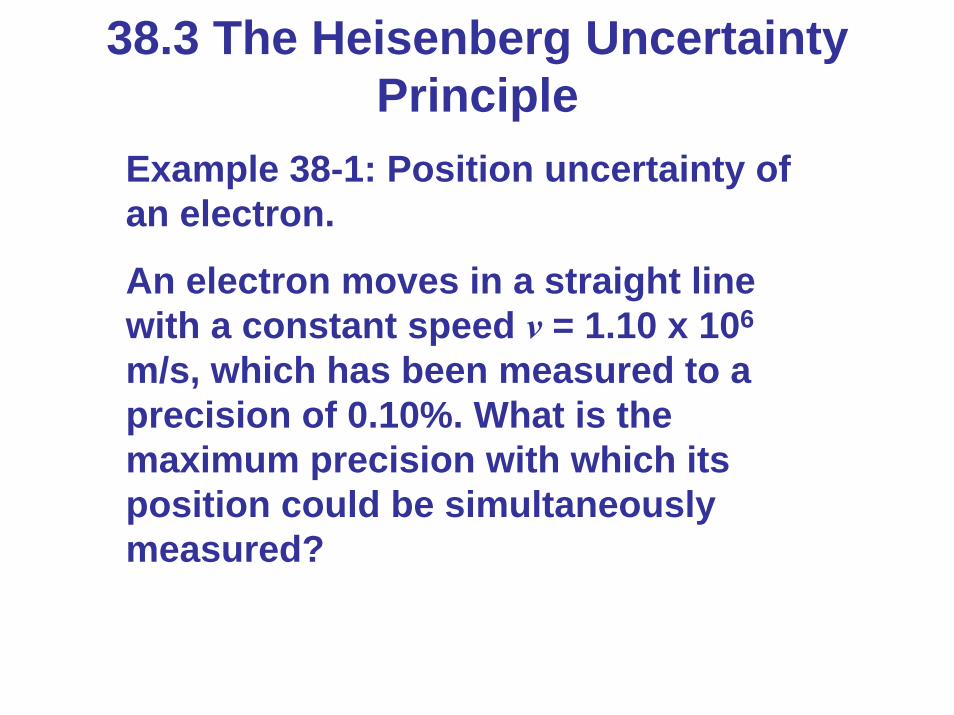
Example 38-1: Position uncertainty of an electron.

An electron moves in a straight line with a constant speed v = 1.10 x 106

m/s, which has been measured to a precision of 0.10%. What is the maximum precision with which its position could be simultaneously measured?

38.3 The Heisenberg Uncertainty Principle

Example 38-2: Position uncertainty of a baseball.

What is the uncertainty in position, imposed by the uncertainty principle, on a 150-g baseball thrown at (93 ± 2) mph = (42 ± 1) m/s?

38.3 The Heisenberg Uncertainty Principle

Example 38-3: J/ψ lifetime calculated.

The J/ψ meson, discovered in 1974, was measured to have an average mass of 3100 MeV/c2 (note the use of energy units since E = mc2) and an intrinsic width of 63 keV/c2. By this we mean that the masses of different J/ψ mesons were actually measured to be slightly different from one another. This mass “width” is related to the very short lifetime of the J/ψ before it decays into other particles. Estimate its lifetime using the uncertainty principle.

The world of Newtonian mechanics is a deterministic one. If you know the forces on an object and its initial velocity, you can predict where it will go.

Quantum mechanics is very different – you can predict what masses of electrons will do, but have no idea what any individual one will do.

38.4 Philosophic Implications; Probability versus Determinism

38.5 The Schrödinger Equation in OneDimension—Time-Independent FormThe Schrödinger equation cannot be derived, just as Newton’s laws cannot. However, we know that it must describe a traveling wave, and that energy must be conserved.

Therefore, the wave function will take the form:

where

38.5 The Schrödinger Equation in OneDimension—Time-Independent Form

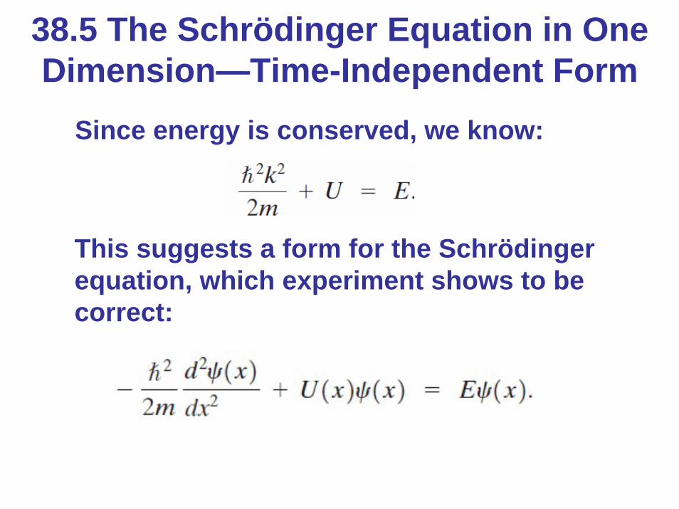
Since energy is conserved, we know:

This suggests a form for the Schrödinger equation, which experiment shows to be correct:

38.5 The Schrödinger Equation in OneDimension—Time-Independent Form

Since the solution to the Schrödinger equation is supposed to represent a single particle, the total probability of finding that particle anywhere in space should equal 1:

When this is true, the wave function is normalized.

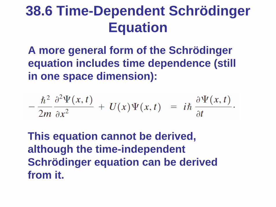
38.6 Time-Dependent SchrödingerEquation

A more general form of the Schrödinger equation includes time dependence (still in one space dimension):

This equation cannot be derived, although the time-independent Schrödinger equation can be derived from it.

38.6 Time-Dependent SchrödingerEquation

Writing

we find that the Schrödinger equation can be separated – its time- and space-dependent parts can be solved for separately.

38.6 Time-Dependent SchrödingerEquation

The time dependence can be found easily; it is:

This function has an absolute value of 1; it does not affect the probability density in space.

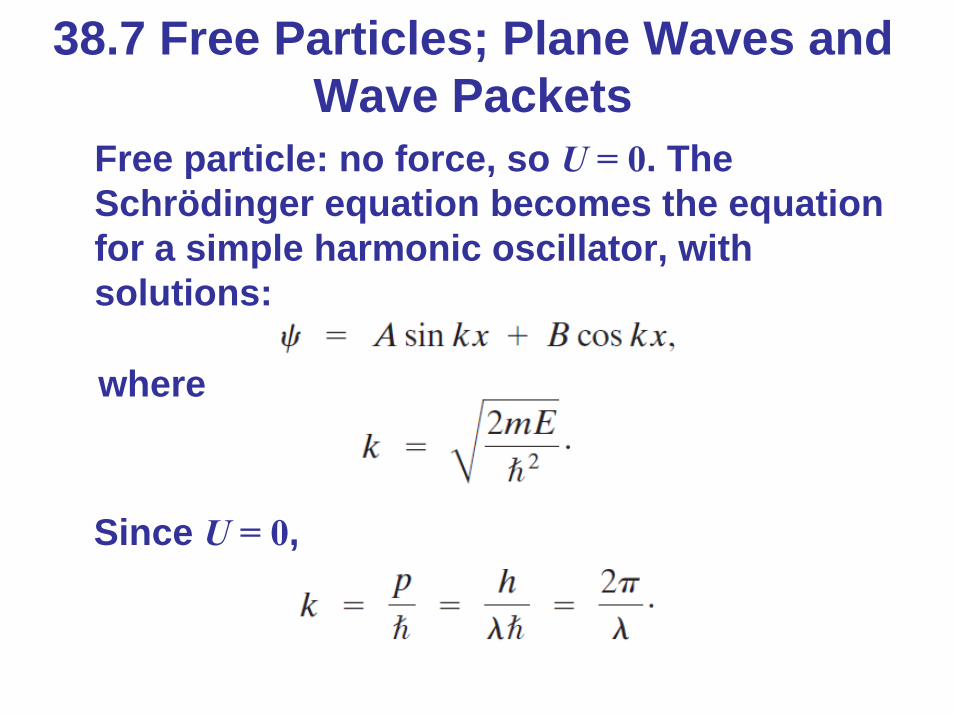
38.7 Free Particles; Plane Waves and Wave Packets

Free particle: no force, so U = 0. The Schrödinger equation becomes the equation for a simple harmonic oscillator, with solutions:

Since U = 0,

where

38.7 Free Particles; Plane Waves and Wave Packets

Example 38-4: Free electron.

An electron with energy E = 6.3 eV is in free space (where U = 0).

Find (a) the wavelength λ (in nm) and

(b) the wave function for the electron (assuming B = 0).

38.7 Free Particles; Plane Waves and Wave Packets

The solution for a free particle is a plane wave, as shown in part (a) of the figure; more realistic is a wave packet, as shown in part (b). The wave packet has both a range of momenta and a finite uncertainty in width.

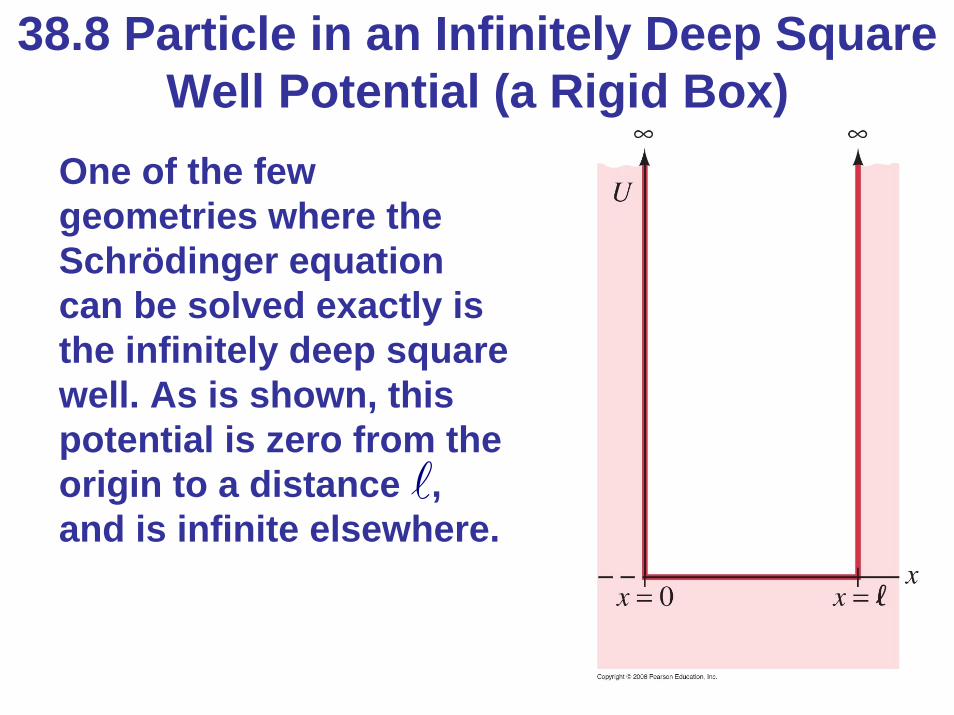
38.8 Particle in an Infinitely Deep SquareWell Potential (a Rigid Box)

One of the few geometries where the Schrödinger equation can be solved exactly is the infinitely deep square well. As is shown, this potential is zero from the origin to a distance , and is infinite elsewhere.

38.8 Particle in an Infinitely Deep SquareWell Potential (a Rigid Box)

The solution for the region between the walls is that of a free particle:

Requiring that ψ = 0 at x = 0 and x = gives B = 0 and k = nπ/ . This means that the energy is limited to the values:

38.8 Particle in an Infinitely Deep SquareWell Potential (a Rigid Box)

These plots show the energy levels, wave function, and probability distribution for several values of n.

38.8 Particle in an Infinitely Deep SquareWell Potential (a Rigid Box)

Example 38-5: Electron in an infinite potential well.

(a) Calculate the three lowest energy levels for an electron trapped in an infinitely deep square well potential of width = 1.00 x 10-10 m (about the diameter of a hydrogen atom in its ground state). (b) If a photon were emitted when the electron jumps from the n = 2 state to the n = 1 state, what would its wavelength be?

38.8 Particle in an Infinitely Deep SquareWell Potential (a Rigid Box)

Example 38-6: Calculating a normalization constant .

Show that the normalization constant A for all wave functions describing a particle in an infinite potential well of width has a value of:

2 / .A =

38.8 Particle in an Infinitely Deep SquareWell Potential (a Rigid Box)

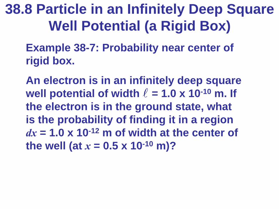
Example 38-7: Probability near center of rigid box.

An electron is in an infinitely deep square well potential of width = 1.0 x 10-10 m. If the electron is in the ground state, what is the probability of finding it in a region dx = 1.0 x 10-12 m of width at the center of the well (at x = 0.5 x 10-10 m)?

38.8 Particle in an Infinitely Deep SquareWell Potential (a Rigid Box)

Example 38-8: Probability of e- in ¼ of box.

Determine the probability of finding an electron in the left quarter of a rigid box—i.e., between one wall at x = 0 and position x = /4. Assume the electron is in the ground state.

38.8 Particle in an Infinitely Deep SquareWell Potential (a Rigid Box)

Example 38-9: Most likely and average positions.

Two quantities that we often want to know are the most likely position of the particle and the average position of the particle. Consider the electron in the box of width = 1.00 x 10-10 m in the first excited state n = 2. (a) What is its most likely position? (b) What is its average position?

38.8 Particle in an Infinitely Deep SquareWell Potential (a Rigid Box)

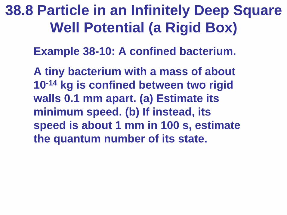
Example 38-10: A confined bacterium.

A tiny bacterium with a mass of about 10-14 kg is confined between two rigid walls 0.1 mm apart. (a) Estimate its minimum speed. (b) If instead, its speed is about 1 mm in 100 s, estimate the quantum number of its state.

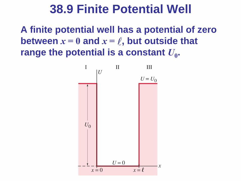
38.9 Finite Potential WellA finite potential well has a potential of zero between x = 0 and x = , but outside that range the potential is a constant U0.

38.9 Finite Potential WellThe potential outside the well is no longer zero; it falls off exponentially.

The wave function in the well is different than that outside it; we require that both the wave function and its first derivative be equal at the position of each wall (so it is continuous and smooth), and that the wave function be normalized.

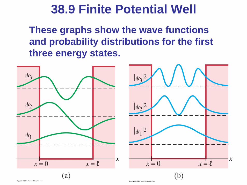
38.9 Finite Potential WellThese graphs show the wave functions and probability distributions for the first three energy states.

Figure 38-13a goes here.

Figure 38-13b goes here.

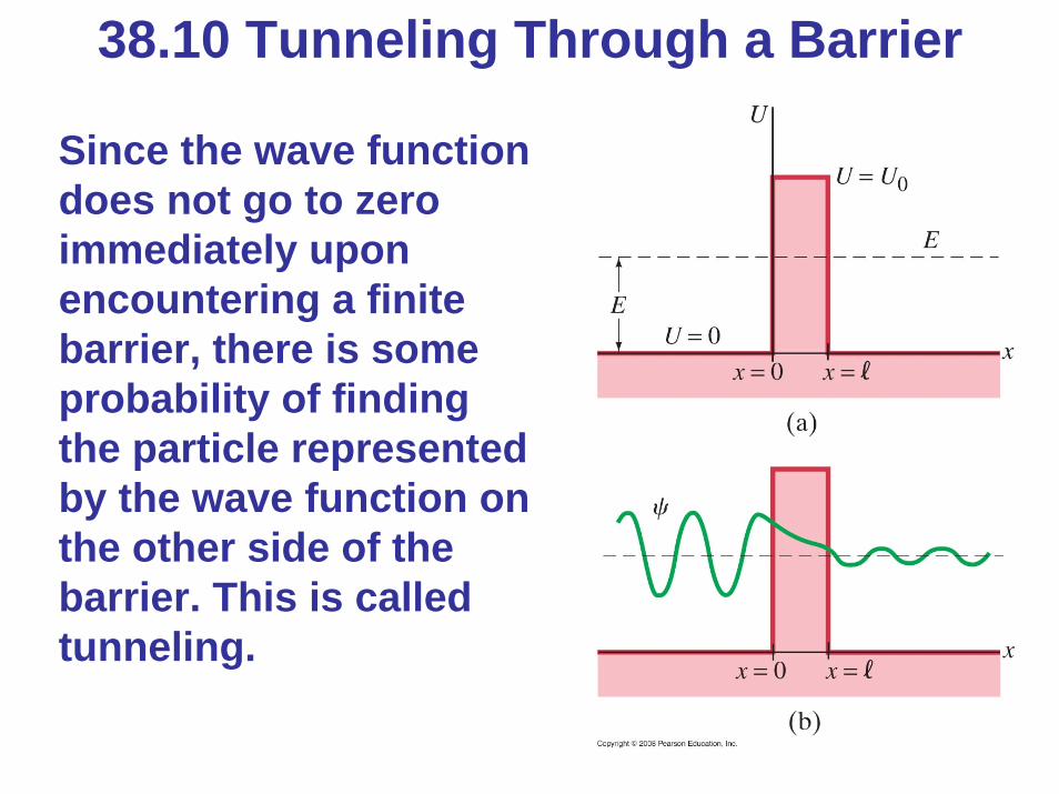
38.10 Tunneling Through a Barrier

Since the wave function does not go to zero immediately upon encountering a finite barrier, there is some probability of finding the particle represented by the wave function on the other side of the barrier. This is called tunneling.

Figure 38-15 goes here.

38.10 Tunneling Through a Barrier

The probability that a particle tunnels through a barrier can be expressed as a transmission coefficient, T, and a reflection coefficient, R (where T + R = 1). If T is small,

The smaller E is with respect to U0, the smaller the probability that the particle will tunnel through the barrier.

38.10 Tunneling Through a Barrier

Example 38-11: Barrier penetration.

A 50-eV electron approaches a square barrier 70 eV high and (a) 1.0 nm thick, (b) 0.10 nm thick. What is the probability that the electron will tunnel through?

38.10 Tunneling Through a BarrierAlpha decay is a tunneling process; this is why alpha decay lifetimes are so variable.

Scanning tunneling microscopes image the surface of a material by moving so as to keep the tunneling current constant. In doing so, they map an image of the surface.

VIDEO: QUANTUM MECHANICS

• Quantum mechanics is the basic theory at the atomic level; it is statistical rather than deterministic

• Heisenberg uncertainty principle:

Summary of Chapter 38

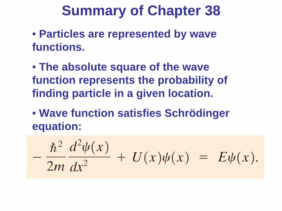
Summary of Chapter 38• Particles are represented by wave functions.

• The absolute square of the wave function represents the probability of finding particle in a given location.

• Wave function satisfies Schrödinger equation:

Equation 38-5 goes here.

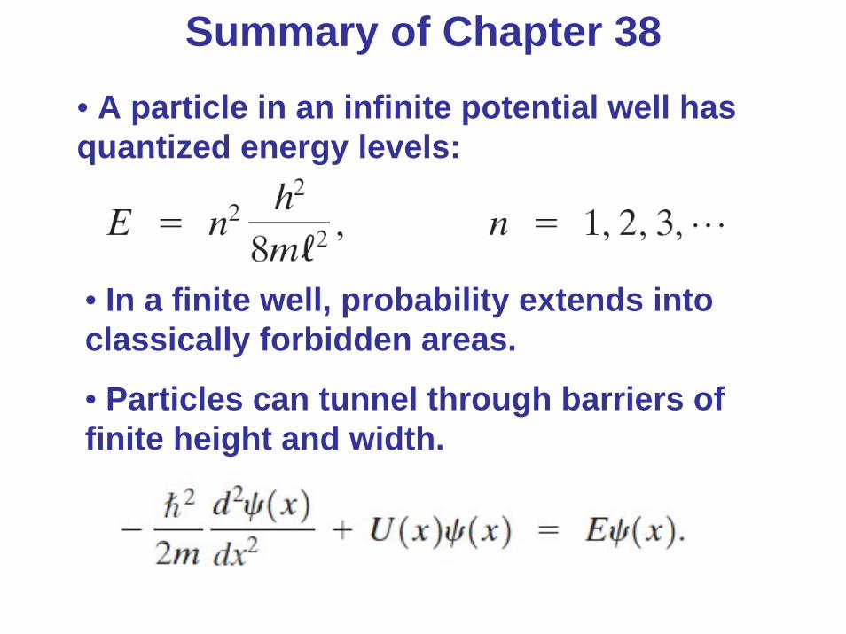
Summary of Chapter 38• A particle in an infinite potential well has quantized energy levels:

Equation 38-13 goes here.

• In a finite well, probability extends into classically forbidden areas.

• Particles can tunnel through barriers of finite height and width.