Chapter 3

The Importance of Forecasting in POM

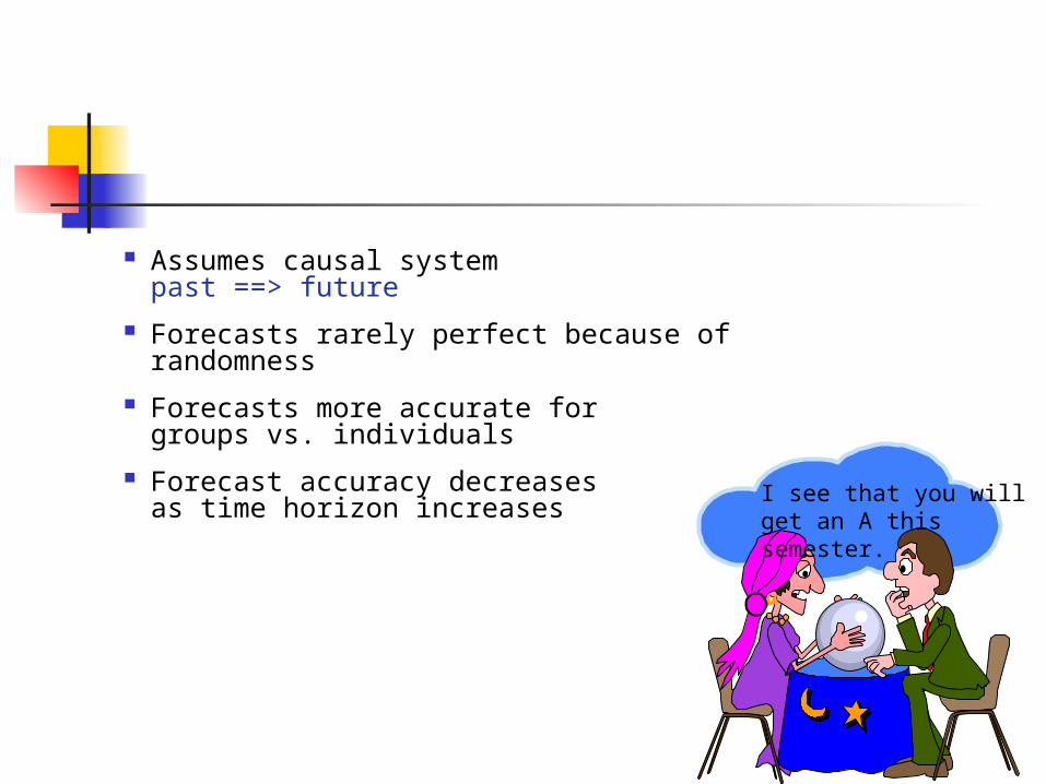
Assumes causal systempast ==> future

Forecasts rarely perfect because of randomness Forecasts more accurate for

groups vs. individuals Forecast accuracy decreases

as time horizon increases I see that you willget an A this semester.

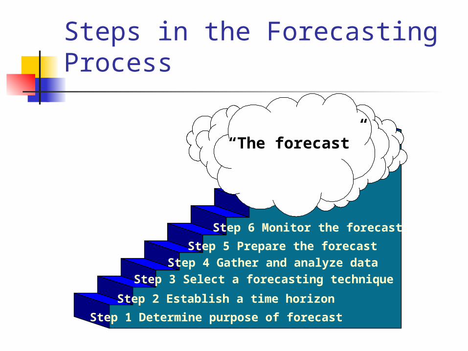
Steps in the Forecasting Process

Step 1 Determine purpose of forecast

Step 2 Establish a time horizon

Step 3 Select a forecasting technique

Step 4 Gather and analyze data

Step 5 Prepare the forecast

Step 6 Monitor the forecast

“The forecast”

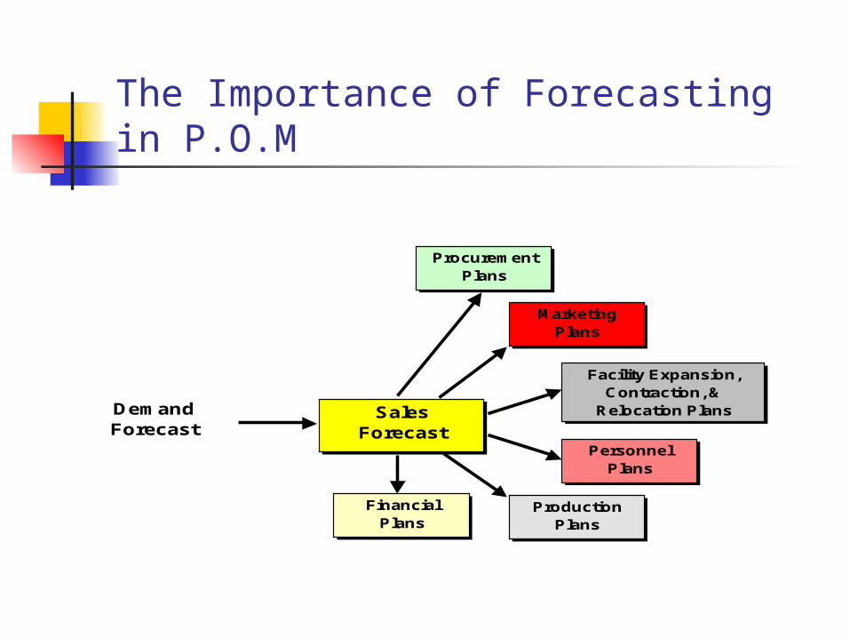
The Importance of Forecasting in P.O.M

DemandForecast

Sales Forecast

Financial Plans

ProductionPlans

Personnel Plans

Facility Expansion,Contraction, &

Relocation Plans

MarketingPlans

ProcurementPlans

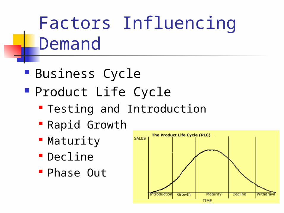
Factors Influencing Demand

Business Cycle Product Life Cycle

Testing and Introduction Rapid Growth Maturity Decline Phase Out

Factors Influencing Demand Other Factors

Competitor’s efforts and prices Customer’s confidence and attitude

Who makes the sales forecast?

Sales Personnel 32%

Marketing Personnel 29%

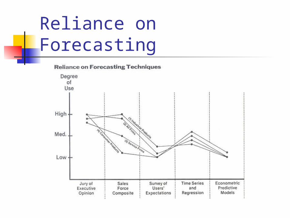
Reliance on Forecasting

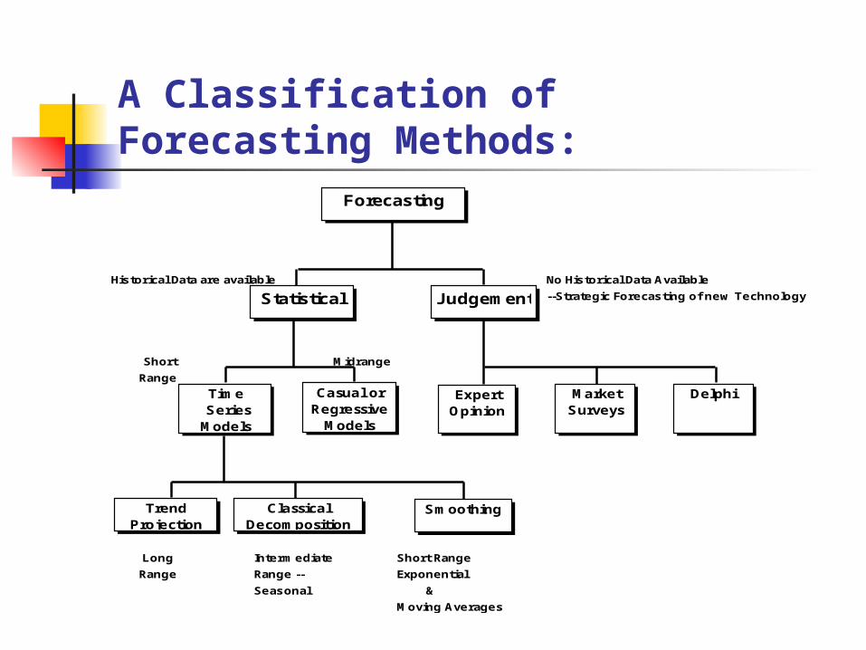
A Classification of Forecasting Methods:

Historical Data are available No Historical Data Available

--Strategic Forecasting of new Technology

Short Midrange

Range

Long Intermediate Short Range

Range Range -- Exponential

Seasonal &

Moving Averages

Forecasting

Statistical Judgement

Time SeriesModels

Casual or Regressive

Models

TrendProjection

ClassicalDecomposition

Smoothing

ExpertOpinion

MarketSurveys

Delphi

Judgmental Forecasts

Executive opinions Sales force opinions Consumer surveys Outside opinion Delphi method

Opinions of managers and staff Achieves a consensus forecast

Statistical Forecasting: Time Series

Model

In Statistical Forecasting, we assume that the actual value of the time series we are trying to forecast consists of a pattern plus some random error.

Time Series Value = Pattern ± Random Error

ActualObservations

1 22 33 44 53 4

1.5 2.53 4

3.5 4.52 31 23 44 55 68 97 86 7

0

1

2

3

4

5

6

7

8

9

10

1 2 3 4 5 6 7 8 9 10 11 12 13 14 15 16

Time

Va

lue

Pattern

Random Error

Actual Observations

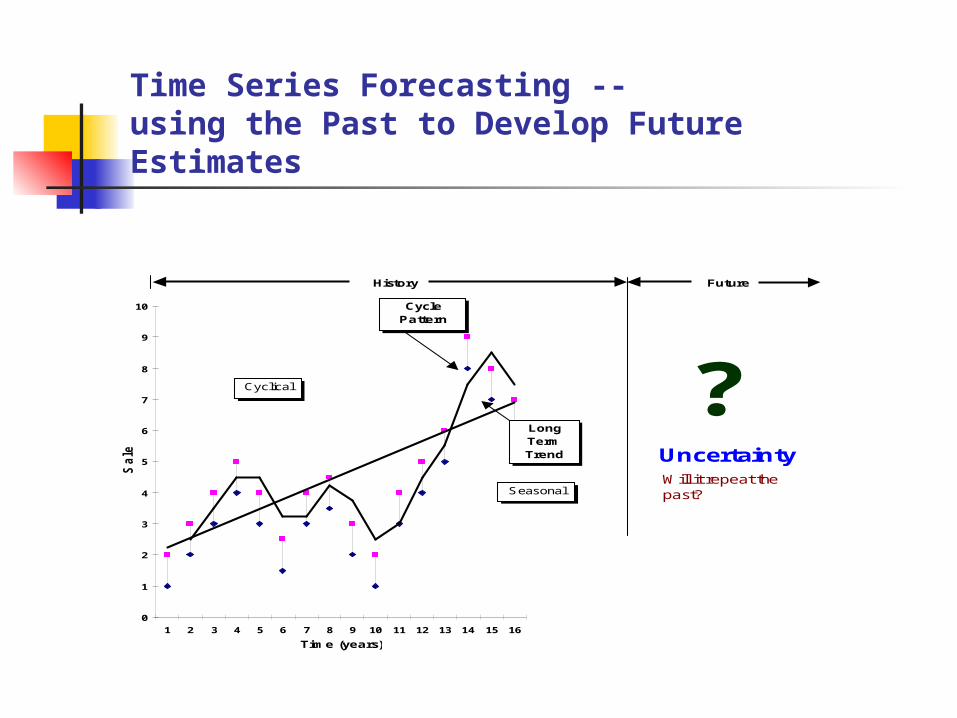
Time Series Forecasting --using the Past to Develop Future Estimates

History Future

0

1

2

3

4

5

6

7

8

9

10

1 2 3 4 5 6 7 8 9 10 11 12 13 14 15 16

Time (years)

Sale

s

Cycle Pattern

LongTermTrend

?UncertaintyWill it repeat the past?Seasonal

Cyclical

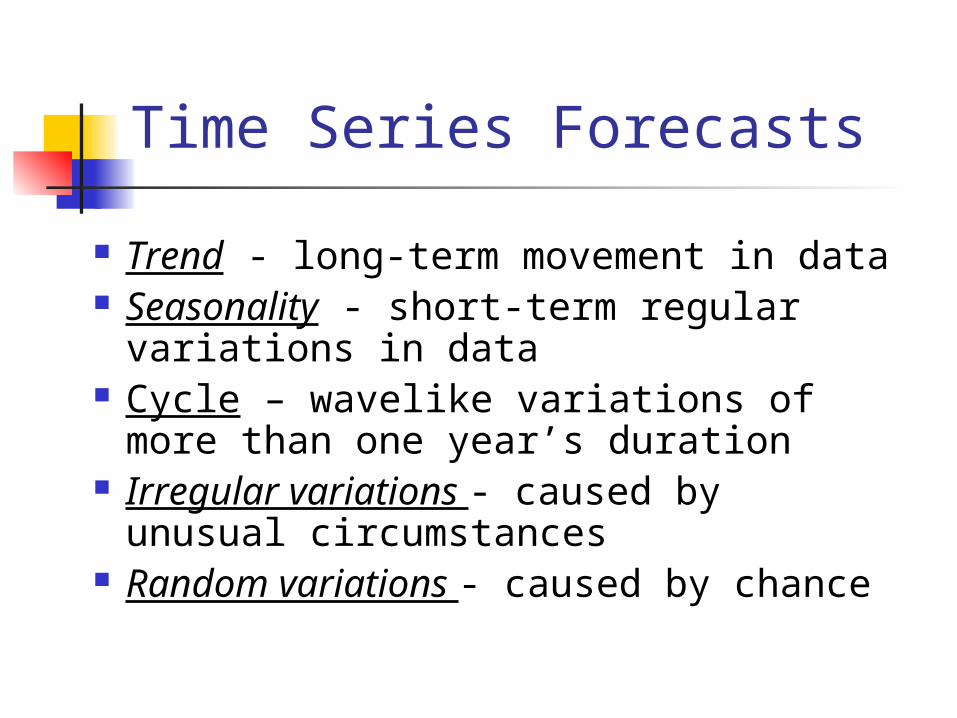
Time Series Forecasts

Trend - long-term movement in data Seasonality - short-term regular

variations in data Cycle – wavelike variations of more

than one year’s duration Irregular variations - caused by

unusual circumstances Random variations - caused by

chance

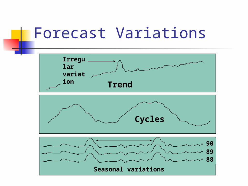
Forecast Variations

Trend

Irregularvariation

Seasonal variations

908988

Cycles

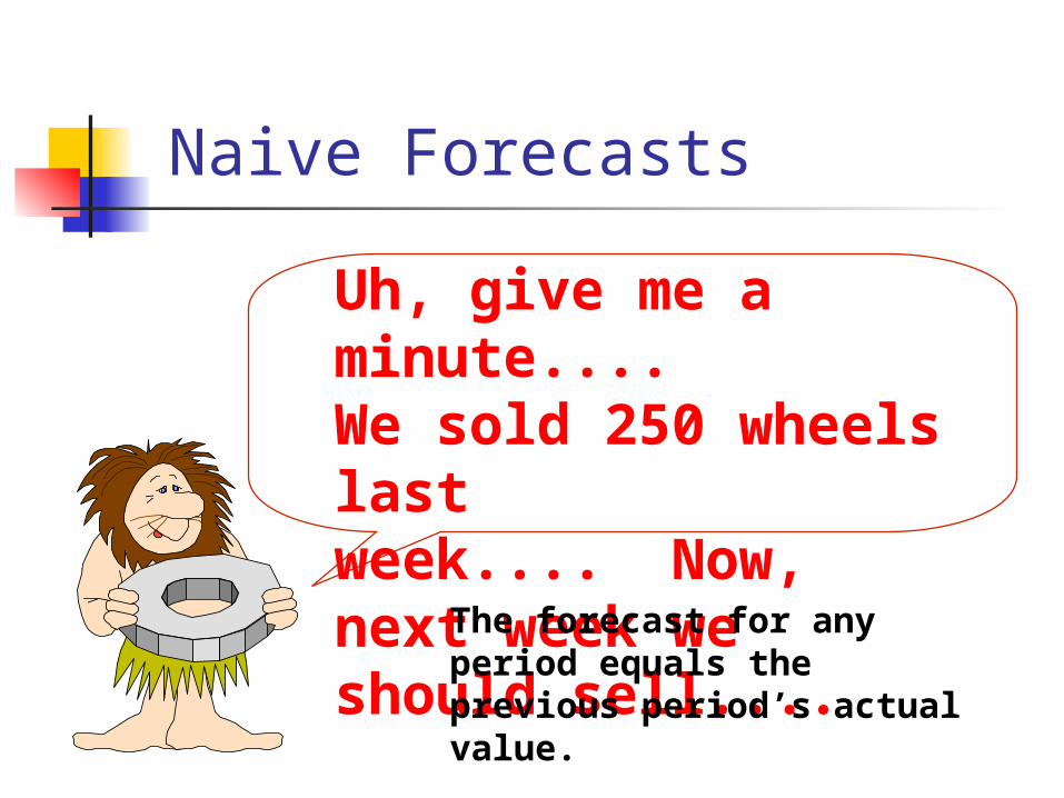
Naive Forecasts

Uh, give me a minute.... We sold 250 wheels lastweek.... Now, next week we should sell....

The forecast for any period equals the previous period’s actual value.

Simple to use Virtually no cost Quick and easy to prepare Data analysis is nonexistent Easily understandable Cannot provide high accuracy Can be a standard for accuracy

Naïve Forecasts

Stable time series data F(t) = A(t-1)

Seasonal variations F(t) = A(t-n)

Data with trends F(t) = A(t-1) + (A(t-1) – A(t-2))

Uses for Naïve Forecasts

Short Run Forecasts Moving Average Method Exponential Smoothing

Moving Average Method This method consists of computing an

average of the most recent n data values in the time series. This average is then used as a forecast for the next period.

Moving average = (most recent n data values)

n Moving average usually tends to eliminate

the seasonal and random components.

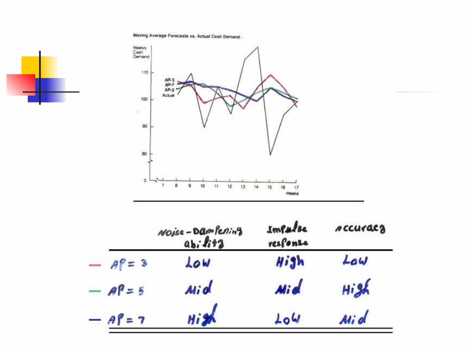
Moving Average Method

The larger the averaging period, n, the smoother the forecast.

The ultimate selection of an averaging period would depend upon management needs.

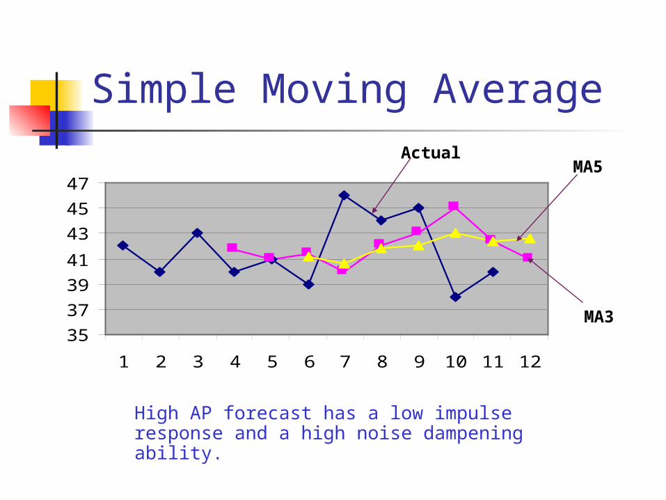
Simple Moving Average

35

37

39

41

43

45

47

1 2 3 4 5 6 7 8 9 10 11 12

Actual

MA3

MA5

High AP forecast has a low impulse response and a high noise dampening ability.

Weighted Moving Average Method

Weighted moving average – More recent values in a series are given more weight in computing the forecast.

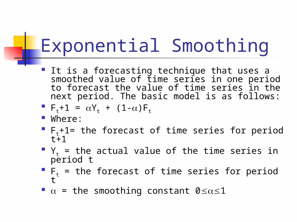
Exponential Smoothing It is a forecasting technique that uses a

smoothed value of time series in one period to forecast the value of time series in the next period. The basic model is as follows:

Ft+1 = Yt + (1-)Ft Where: Ft+1= the forecast of time series for period

t+1 Yt = the actual value of the time series in

period t Ft = the forecast of time series for period t = the smoothing constant 01

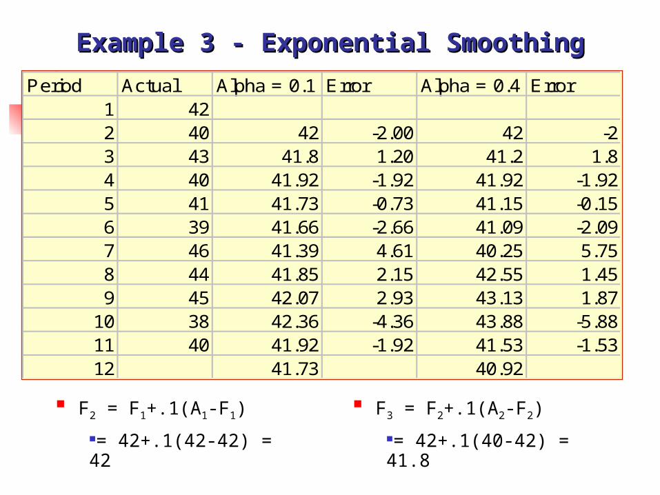
Period Actual Alpha = 0.1 Error Alpha = 0.4 Error1 422 40 42 -2.00 42 -23 43 41.8 1.20 41.2 1.84 40 41.92 -1.92 41.92 -1.925 41 41.73 -0.73 41.15 -0.156 39 41.66 -2.66 41.09 -2.097 46 41.39 4.61 40.25 5.758 44 41.85 2.15 42.55 1.459 45 42.07 2.93 43.13 1.87

10 38 42.36 -4.36 43.88 -5.8811 40 41.92 -1.92 41.53 -1.5312 41.73 40.92

Example 3 - Exponential SmoothingExample 3 - Exponential Smoothing

F2 = F1+.1(A1-F1)

= 42+.1(42-42) = 42

F3 = F2+.1(A2-F2)

= 42+.1(40-42) = 41.8

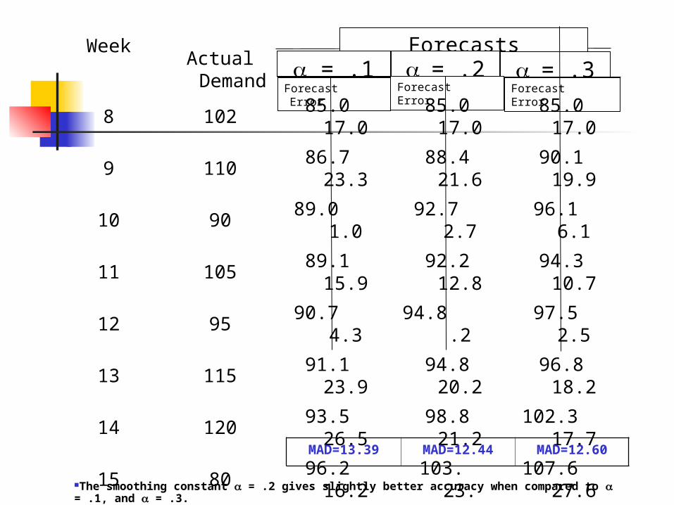
Forecasts = .1 = .2 = .3

Forecast Error Forecast Error Forecast Error

Week

8 102 85.0 17.0 85.0 17.0 85.0 17.0

9 110 86.7 23.3 88.4 21.6 90.1 19.9

10 90 89.0 1.0 92.7 2.7 96.1 6.1

11 105 89.1 15.9 92.2 12.8 94.3 10.7

12 95 90.7 4.3 94.8 .2 97.5 2.5

13 115 91.1 23.9 94.8 20.2 96.8 18.2

14 120 93.5 26.5 98.8 21.2102.3

17.7

15 80 96.2 16.2 103. 23.107.6

27.6

16 95 94.6 .4 98.4 3.4 99.3 4.3

17 100 94.6 5.4 97.7 2.3 98.0 2.0

Total Errors

133.9 124.4 126

Actual Deman

d

MAD=13.39 MAD=12.44 MAD=12.60

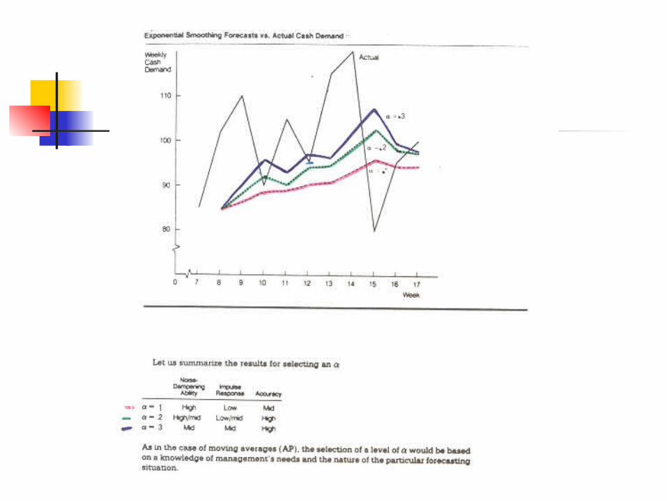
The smoothing constant = .2 gives slightly better accuracy when compared to = .1, and = .3.

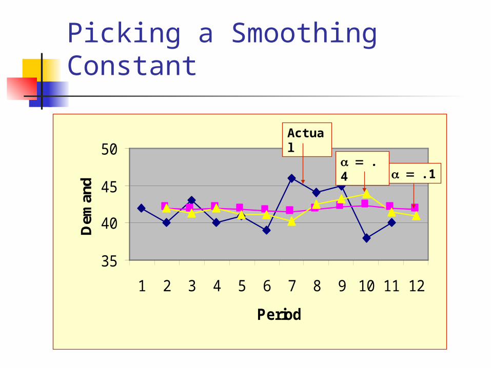
Picking a Smoothing Constant

35

40

45

50

1 2 3 4 5 6 7 8 9 10 11 12

Period

Dem

and .1

.4

Actual

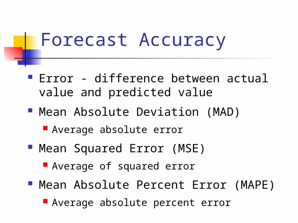
Forecast Accuracy

Error - difference between actual value and predicted value

Mean Absolute Deviation (MAD) Average absolute error

Mean Squared Error (MSE) Average of squared error

Mean Absolute Percent Error (MAPE) Average absolute percent error

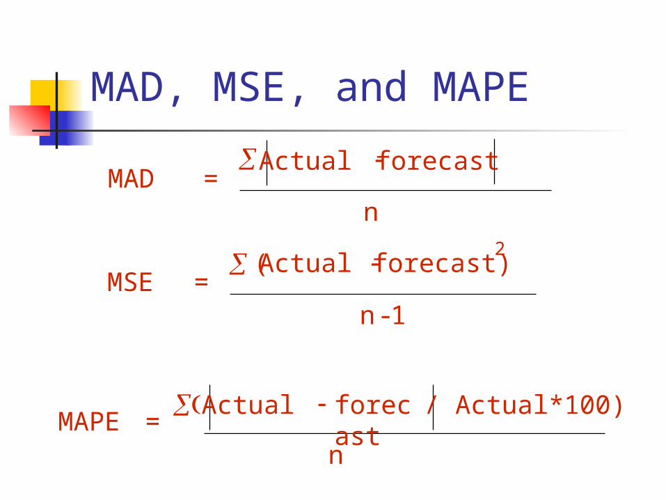
MAD, MSE, and MAPE

MAD = Actual forecast

n

MSE = Actual forecast)

-1

2

n

(

MAPE = Actual forecas

t

n

/ Actual*100)

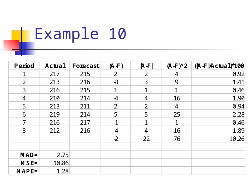
Example 10

Period Actual Forecast (A-F) |A-F| (A-F)^2 (|A-F|/Actual)*1001 217 215 2 2 4 0.922 213 216 -3 3 9 1.413 216 215 1 1 1 0.464 210 214 -4 4 16 1.905 213 211 2 2 4 0.946 219 214 5 5 25 2.287 216 217 -1 1 1 0.468 212 216 -4 4 16 1.89

-2 22 76 10.26

MAD= 2.75MSE= 10.86

MAPE= 1.28

Controlling the Forecast

Control chart A visual tool for monitoring forecast

errors Used to detect non-randomness in

errors Forecasting errors are in control if

All errors are within the control limits No patterns, such as trends or cycles,

are present

Sources of Forecast errors

Model may be inadequate Irregular variations Incorrect use of forecasting

technique

Tracking Signal

Tracking signal = (Actual-forecast)

MAD

•Tracking signal

–Ratio of cumulative error to MAD

Bias – Persistent tendency for forecasts to beGreater or less than actual values.

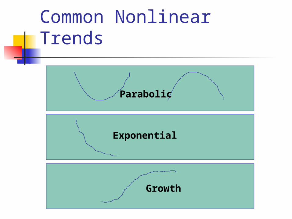
Common Nonlinear Trends

Parabolic

Exponential

Growth

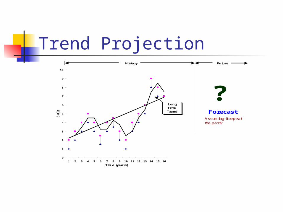
Trend ProjectionHistory Future

0

1

2

3

4

5

6

7

8

9

10

1 2 3 4 5 6 7 8 9 10 11 12 13 14 15 16

Time (years)

Sale

s

LongTermTrend

?Forecast

Assuming it repeat the past?

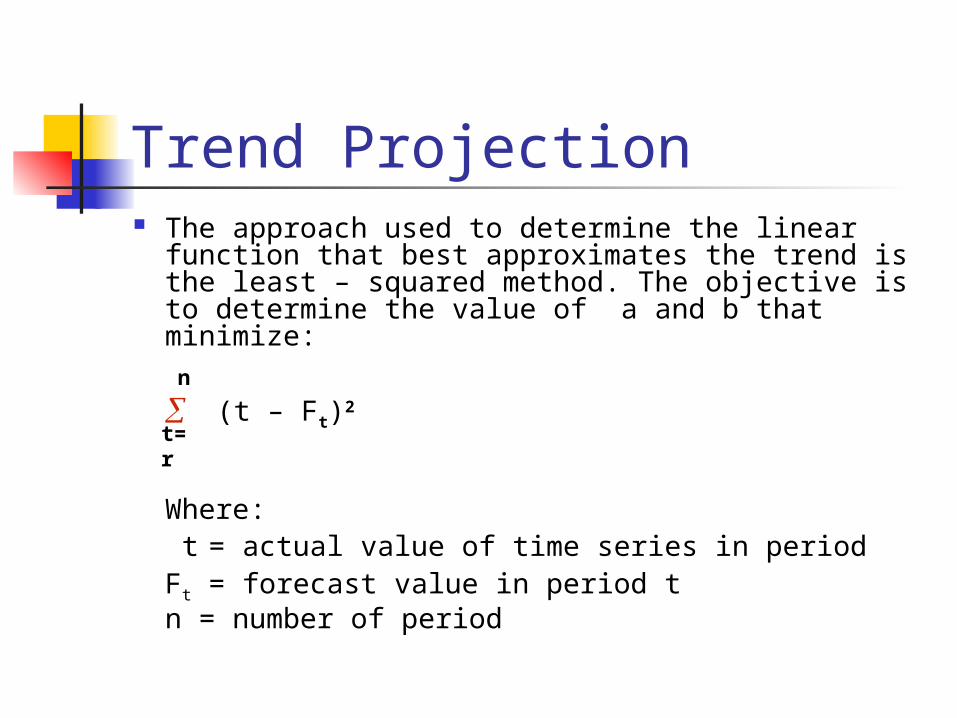
Trend Projection The approach used to determine the linear

function that best approximates the trend is the least – squared method. The objective is to determine the value of a and b that minimize:

(t – Ft)2

Where: t = actual value of time series in period Ft = forecast value in period t n = number of period

n

t=r

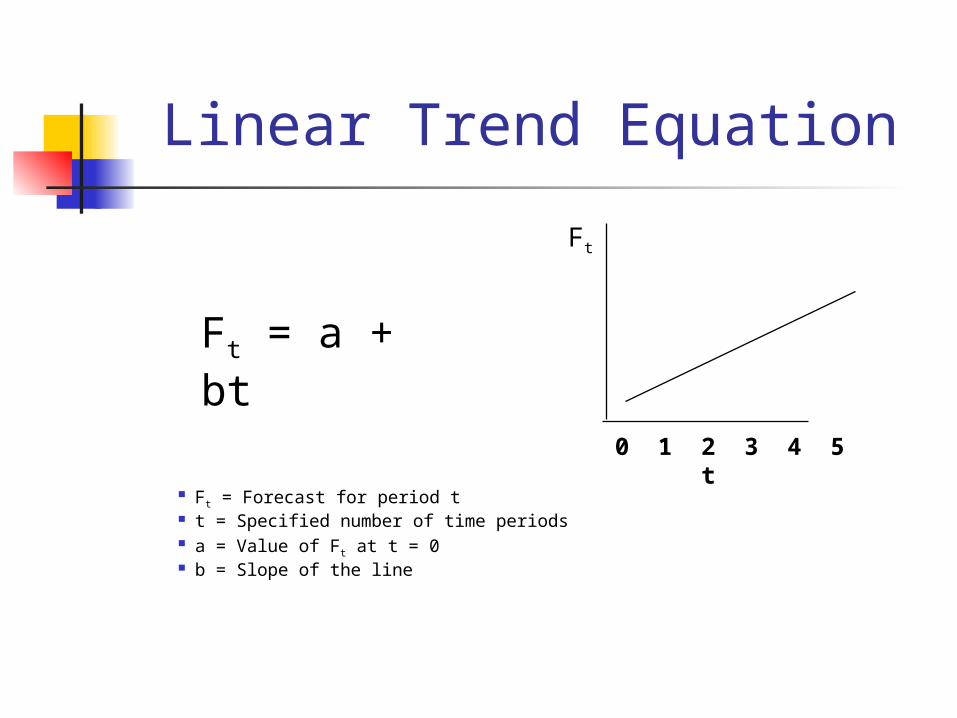
Linear Trend Equation

Ft = Forecast for period t t = Specified number of time periods a = Value of Ft at t = 0 b = Slope of the line

Ft = a + bt

0 1 2 3 4 5 t

Ft

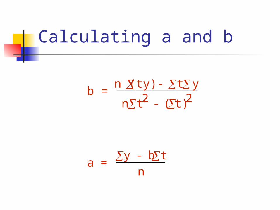
Calculating a and b

b = n (ty) - t y

n t2 - ( t)2

a = y - b t

n

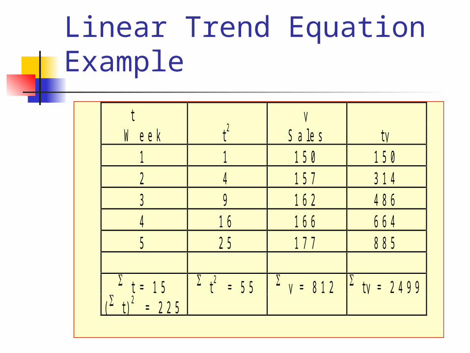
Linear Trend Equation Example

t yW e e k t 2 S a l e s t y

1 1 1 5 0 1 5 02 4 1 5 7 3 1 43 9 1 6 2 4 8 64 1 6 1 6 6 6 6 45 2 5 1 7 7 8 8 5

t = 1 5 t 2 = 5 5 y = 8 1 2 t y = 2 4 9 9( t ) 2 = 2 2 5

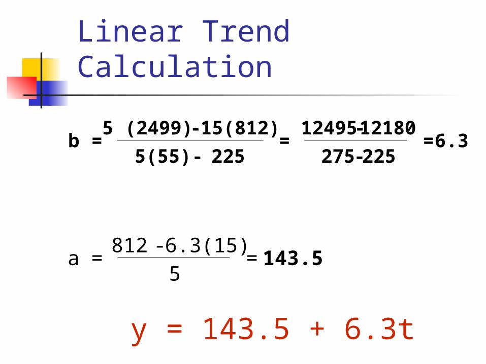
Linear Trend Calculation

y = 143.5 + 6.3t

a = 812 - 6.3(15)

5 =

b = 5 (2499) - 15(812)

5(55) - 225 =

12495-12180

275 -225 = 6.3

143.5

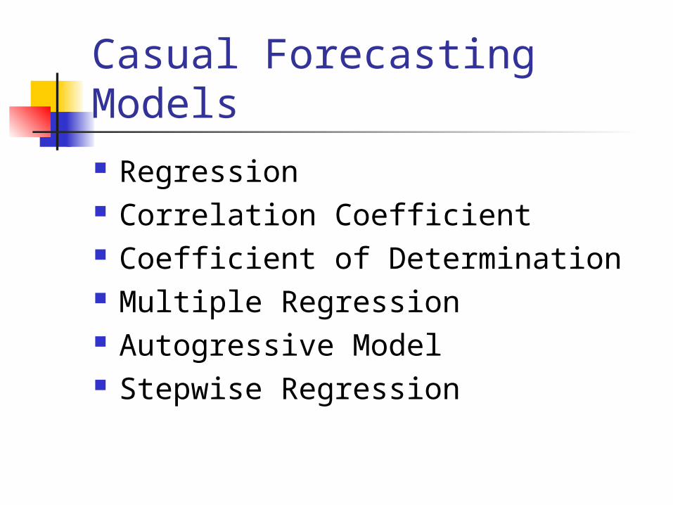
Casual Forecasting Models Regression Correlation Coefficient Coefficient of Determination Multiple Regression Autogressive Model Stepwise Regression

Associative Forecasting

Regression - technique for fitting a line to a set of points

Least squares line - minimizes sum of squared deviations around the line

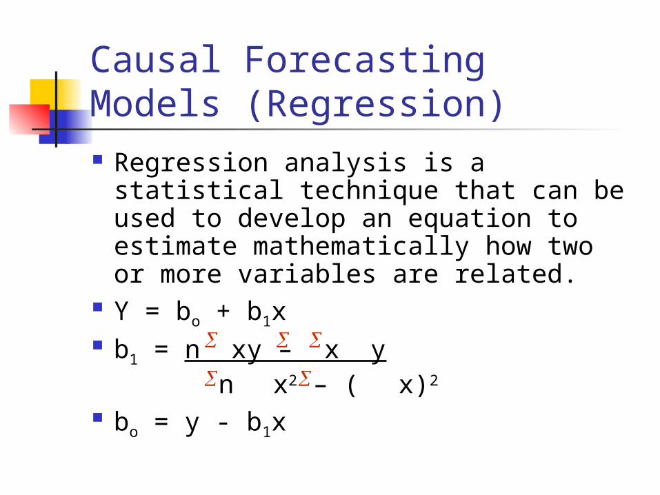
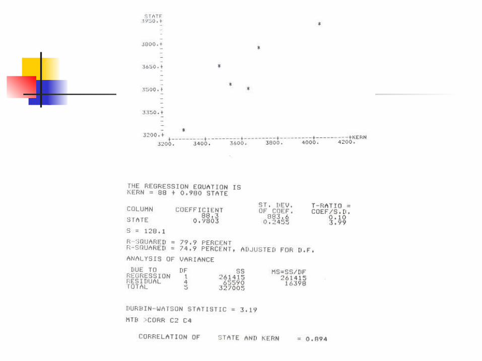
Causal Forecasting Models (Regression) Regression analysis is a statistical

technique that can be used to develop an equation to estimate mathematically how two or more variables are related.

Y = bo + b1x b1 = n xy – x y nx2 – (x)2

bo = y - b1x

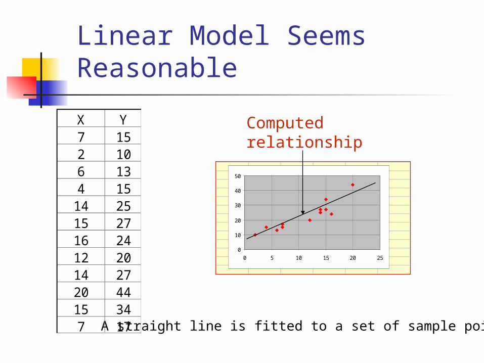
Linear Model Seems Reasonable

A straight line is fitted to a set of sample points.

0

10

20

30

40

50

0 5 10 15 20 25

X Y7 152 106 134 15

14 2515 2716 2412 2014 2720 4415 347 17

Computedrelationship

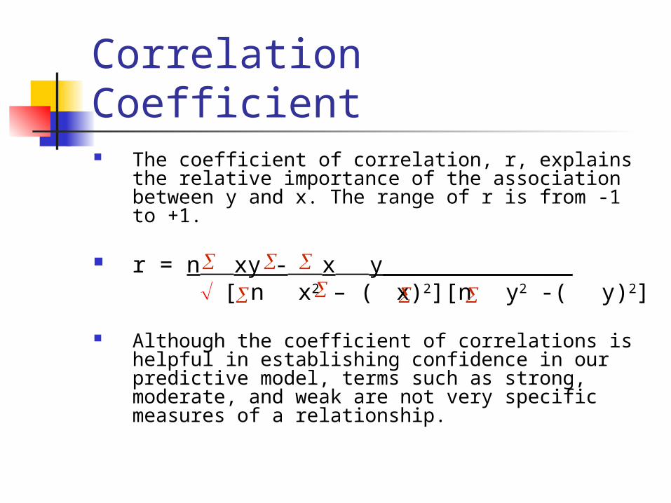
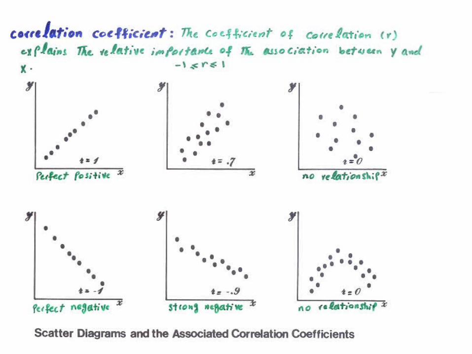
Correlation Coefficient The coefficient of correlation, r, explains the

relative importance of the association between y and x. The range of r is from -1 to +1.

r = nxy -xy______________ [ nx2 – (x)2][ny2 -(y)2]

Although the coefficient of correlations is helpful in establishing confidence in our predictive model, terms such as strong, moderate, and weak are not very specific measures of a relationship.

Coefficient of Determination The coefficient of determination, r2,

is the square of the coefficient of correlation.

This measure indicates the percent of variation in y that is explained by x.

Multiple Regression Multiregression analysis is used when two

or more independent variables are incorporated into the analysis. In forecasting the sale of refrigerators, we

might select independent variable such as: Y= annual sales in thousands of units X1 = price in period t X2 = total industry sales in period t-1 X3 = number of building permits for new

houses in period t-1

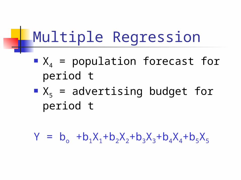
Multiple Regression X4 = population forecast for period

t X5 = advertising budget for period

t

Y = bo +b1X1+b2X2+b3X3+b4X4+b5X5

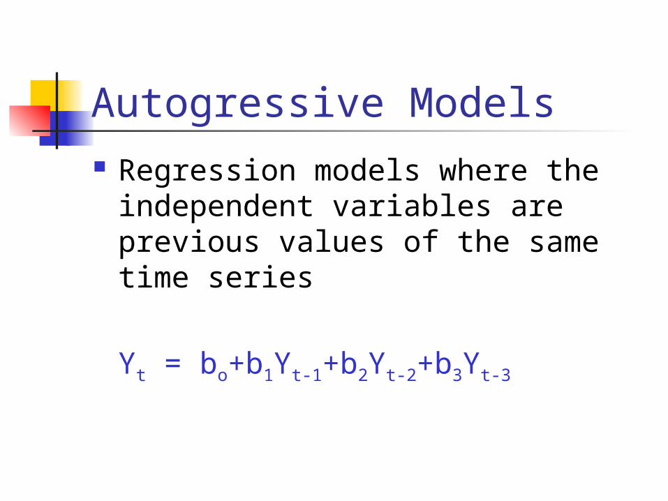
Autogressive Models Regression models where the

independent variables are previous values of the same time series

Yt = bo+b1Yt-1+b2Yt-2+b3Yt-3

Stepwise Regression In regular multiple regression

analysis, all the independent variables are entered into the analysis concurrently.

In stepwise regression analysis, independent variables will be selected for entry into the analysis on the basis of their explanatory (discriminatory) power.

Choosing a Forecasting Technique

No single technique works in every situation

Two most important factors Cost Accuracy

Other factors include the availability of: Historical data Computers Time needed to gather and analyze the data Forecast horizon

Exponential SmoothingExponential Smoothing

Linear Trend EquationLinear Trend Equation

Simple Linear RegressionSimple Linear Regression