Embed Size (px)
Citation preview

64
Chapter 3 – Probability We have completed our study of Descriptive Statistics and are headed for Statistical Inference. Before we get there, we need to learn a little bit about probability.
3.1 – Basic Concepts of Probability 1. Probability – Probability is a numerical measure of the likelihood of some event occurring. It is measured on
a scale from 0 to 1: 0 ≤ 𝑃𝑟𝑜𝑏𝑎𝑏𝑖𝑙𝑖𝑡𝑦 ≤ 1. The smaller (larger) the probability the less (more) likely it is that the event will occur. An event with probability 0 never occurs; an event with probability 1 always occurs. Mostly, probabilities are somewhere between these two extremes.
2. Example: Consider flipping a fair coin. There are two possible outcomes and we generally assume that they are equally likely. Thus, 𝑃(𝑇) = 𝑃(𝐻) = 1/2
3. Definitions:
a. Experiment – a repeatable process whose output varies over a set of possible outcomes. b. Sample space – The set of all possible experimental outcomes.
4. Examples: a. Experiment: flip a coin
Sample space: {H, T}
b. Experiment: flip two coins Sample space: {TT, TH, HT, HH}
Sometimes a tree diagram is useful to enumerate a sample space:
c. Experiment: roll a die
Sample space: {1, 2, 3, 4, 5, 6} 5. Simple Sample Space – Suppose there are 𝑛 outcomes in a sample space and they
are all equally likely then the probability of each outcome is the same, 1/𝑛.
6. Examples a. Experiment: Roll a six-sided die.
𝑃(1) = 𝑃(2) = 𝑃(3) = 𝑃(4) = 𝑃(5) = 𝑃(6) = 1/6
b. Experiment: Roll two six-sided dice.

65
How many outcomes are there? 36 = 6*6
Are they all equally likely? Yes.
𝑃(1,1) = 𝑃(1,2) = 𝑃(2,1) = 𝑃(1,3) = ⋯ = 𝑃(6,6) = 1/36
c. Experiment: Flip two coins
d. Experiment: Pick a person at random from a room with these people in it: A, B, C, D. Sample space: {A, B, C, D} What is the probability that C is picked? Answer: 1/4
e. Experiment: Pick two people from A, B, C, D to form a committee. This experiment is a little different in two ways. First, once we pick the first person, they can’t be picked again. Second, the order people are picked doesn’t matter. For example picking A first and then B is the same as picking B first and then A. if we draw the tree diagram as shown on the right, then the sample space is:
Sample space: {AB, AC, AD, BA, BC, BD, CA, CB, CD, DA, DB, DC } where each outcome has probability 1/12. However, noticing that the order doesn’t matter, the sample space can be written:
Sample space: {AB, AC, AD, BC, BD, CD } where each outcome has probability 1/6.

66
7. Probability is the mathematical theory that Statistical Inference is based upon. In this chapter, we learn just enough probability here to give us some insight into how inference works and that might be useful in other ways. Next, we refine earlier definitions and introduce some notation.
8. Definitions and notation: a. Sample Space – We denote the sample space as the set of all possible outcomes (simple events) to an
experiment, 𝑆 = {𝐸1, 𝐸2, ⋯ , 𝐸𝑛}, where 𝑛 is the number of items in the sample space.
b. Probability Requirements for a given sample space:
All probabilities are between 0 and 1: 0 ≤ 𝑃(𝐸𝑖) ≤ 1, 𝑖 = 1,2, … , 𝑛.
The sum of all probabilities is 1: ∑ 𝑃(𝐸𝑖)𝑛𝑖=1 = 1.
c. Example – Roll a six-sided die. Let: 𝐸𝑖 = face 𝑖 𝑖𝑠 𝑜𝑏𝑠𝑒𝑟𝑣𝑒𝑑. Thus,
𝑆 = {𝐸1, 𝐸2, 𝐸3, 𝐸4, 𝐸5, 𝐸6}, 𝑃(𝐸1) = 𝑃(𝐸2) = 𝑃(𝐸3) = 𝑃(𝐸4) = 𝑃(𝐸5) = 𝑃(𝐸6) = 1/6
and finally, we see that if you add up all the probabilities you get 1:
∑ 𝑃(𝐸𝑖)6𝑖=1 =
1
6+
1
6+
1
6+
1
6+
1
6= 1
3.2 – Events 1. Definitions
a. Simple Event – A simple event is an individual outcome to an experiment.
b. Event – An event is a subset of the sample space which is comprised of a set of simple events.
c. Probability of an Event – The probability of an event is the sum of the probabilities of the simple events
that comprise it. 2. Example – Find the probability of an even outcome when a six-sided die is rolled.
Let A = an even outcome is observed when a die is rolled, A = {E2, E4, E6} = {2,4,6}.
𝑃(𝐴) = 𝑃(2) + 𝑃(4) + 𝑃(6) =1
6+
1
6+
1
6=
3
6=
1
2= 0.5
3. Example – Flip two coins.
a. Find the probability of getting a head and a tail
Let 𝐸 = 𝑎 ℎ𝑒𝑎𝑑 𝑎𝑛𝑑 𝑎 𝑡𝑎𝑖𝑙 𝑎𝑟𝑒 𝑜𝑏𝑠𝑒𝑟𝑣𝑒𝑑 = {𝑇𝐻, 𝐻𝑇}

67
b. Find the probability of getting at least one head.
Let 𝐵 = 𝑎𝑡 𝑙𝑒𝑎𝑠𝑡 𝑜𝑛𝑒 ℎ𝑒𝑎𝑑 = {𝑇𝐻, 𝐻𝑇, 𝐻𝐻}
𝑃(𝐵) = 𝑃(𝑇𝐻) + 𝑃(𝐻𝑇) + 𝑃(𝐻𝐻) =1
4+
1
4+
1
4=
3
4= 0.75
4. Example – Choose a card from a standard deck.
𝑆 = {2𝐻 , 2𝐷 , 2𝐶 , 2𝑆, 3𝐻 , 3𝐷 , 3𝐶 , 3𝑆 , … } a. Find the probability that an ace of hearts was picked. 𝑃(𝐴𝐻) = 1/52.
b. Find the probability that an ace was picked.
Let 𝐴 = 𝑎𝑛 𝑎𝑐𝑒 𝑤𝑎𝑠 𝑝𝑖𝑐𝑘𝑒𝑑 = {𝐴𝐻 , 𝐴𝐷 , 𝐴𝐶 , 𝐴𝑆}
𝑃(𝐴) = 𝑃(𝐴𝐻) + 𝑃(𝐴𝐶) + 𝑃(𝐴𝐷) + 𝑃(𝐴𝑆) =1
52+
1
52+
1
52+
1
52=
4
52=
1
13= 0.077
c. Find the probability that a spade was picked.
Let 𝐵 = 𝑎𝑛 𝑠𝑝𝑎𝑑𝑒 𝑤𝑎𝑠 𝑝𝑖𝑐𝑘𝑒𝑑 = {2𝑆, 3𝑆, … , 𝐾𝑆, 𝐴𝑆}
𝑃(𝐵) = 𝑃(2𝑆) + 𝑃(3𝑆) + ⋯ + 𝑃(𝐴𝑆) =1
52+
1
52+ ⋯ +
1
52=
13
52=
1
4= 0.25
d. Find the probability that an ace or a
spade was picked.
Let 𝐶 =𝑎𝑛 𝑎𝑐𝑒 𝑜𝑟 𝑎 𝑠𝑝𝑎𝑑𝑒 𝑤𝑎𝑠 𝑝𝑖𝑐𝑘𝑒𝑑 ={2𝑆, 3𝑆, … , 𝐾𝑆, 𝐴𝑆 , 𝐴𝐻 , 𝐴𝐷 , 𝐴𝐶}
𝑃(𝐶) =16
52=
4
13= 0.308
Note that 𝑃(𝐶) ≠ 𝑃(𝐴) + 𝑃(𝐵)
5. Example – Roll two six-sided die. Find the probability: a. The sum is 5 b. The sum is 9 or more c. The faces are the same

68
6. Example – Flip 4 coins. Find the probability of a. Exactly 2 heads and 2 tails. (the
outcomes shown in green) 𝑃(𝐴) =6
16= 0.375
b. Exactly 3 heads or exactly 3 tails.
𝑃(𝐵) =8
16= 0.5
c. No heads (or equivalently, all tails).
𝑃(𝐶) =1
16= 0.0625
3.3 – Classical Methods of Assigning Probabilities 1. Classical methods of assigning probabilities are based on counting techniques such as the multiplication rule,
combinations, and permutations. We have seen simple examples of counting in the previous section.
2. Multiplication Rule – Suppose we can think of an experiment as a sequence of 𝑆 steps. If there are 𝑛1 ways to do the first step, 𝑛2 ways to do the second step, …, and 𝑛𝑆 ways to do the Sth step then the total number of ways the 𝑆 steps can occur is: 𝑛1 ∗ 𝑛2 ∗ … ∗ 𝑛𝑆.
3. Examples a. Roll 2 dice. How many possibilities are there? 6 ∗ 6 = 36
b. Flip 4 coins. How many possibilities are there? 2 ∗ 2 ∗ 2 ∗ 2 = 16
c. A license plate is composed of 3 letters followed by 3 digits. How many possible license plates are there?
26 ∗ 26 ∗ 26 ∗ 10 ∗ 10 ∗ 10 = 17,576,000
d. A restaurant has 3 meats, 6 vegetables, and 2 deserts. A lunch special is composed of 1 of each. How many different lunch specials are there? 3 ∗ 6 ∗ 2 = 36
4. Combinations – A combination is a way of selecting a number of items from a larger group where the order
of the items does not matter and repeats are not allowed. Suppose there are 𝑛 choices and we want to choose 𝑘 of them (𝑘 ≤ 𝑛) in such a way that the order doesn’t matter. The total number of ways this can be done is:
(𝑛𝑘
) = 𝑛 𝑐ℎ𝑜𝑜𝑠𝑒 𝑘 =𝑛!
𝑘! (𝑛 − 𝑘)!

69
5. Examples
a. How many ways can we pick two people from A, B, C, D to form a committee?
As we noted earlier, the order people are picked doesn’t matter and each person can be picked only once. So, a combination can be used to determine the number of possibilities.
(42
) =4!
2! 2!=
4 ∗ 3 ∗ 2 ∗ 1
(2 ∗ 1) ∗ (2 ∗ 1)= 6
And those possibilities are: {AB, AC, AD, BC, BD, CD }
b. Suppose there are 6 vegetables on a buffet. How many ways can you choose 2 different ones.
(62
) =6!
2! (6 − 2)!=
6!
2! 4!=
6 ∗ 5 ∗ 4!
2! 4!=
6 ∗ 5
2= 15
e. A restaurant has 3 meats, 6 vegetables, and 2 deserts. A lunch special is composed of 1 meat, 2 vegetables and a desert. How many different lunch specials are there? Multiplication rule:
Number of ways to choose a meat
Number of ways to choose 2 vegetables
Number of ways to choose a desert
3 * (62
) * 2
= 3 ∗ 15 ∗ 2 = 90
f. How many ways are there to pick 5 cards from a standard deck? Answer: (525
).
We can work this by hand, or use the calculator to answer this question:
1. Type: 52
2. Press the MATH key
3. Use the right-arrow key to scroll over to PRB, then the down-arrow key to scroll down to nCr. Press Enter.
4. Type: 5 and press Enter.

70
g. Pick 2 cards from a standard deck. How many ways are there to pick 2 Aces? (42
) = 6
e.g. {(𝐴𝐻 , 𝐴𝐷), (𝐴𝐻 , 𝐴𝐶), (𝐴𝐻 , 𝐴𝑆), (𝐴𝐷 , 𝐴𝐶), (𝐴𝐷 , 𝐴𝑆), (𝐴𝐶 , 𝐴𝑆)}
h. Pick 2 cards from a standard deck. How many different 2 card hands are there? (522
) = 1326
i. Pick 2 cards from a standard deck. What is the probability of choosing exactly 2 Aces?
# 𝑤𝑎𝑦𝑠 𝑡𝑜 𝑝𝑖𝑐𝑘 2 𝐴𝑐𝑒𝑠
# 𝑤𝑎𝑦𝑠 𝑡𝑜 𝑝𝑖𝑐𝑘 2 𝑐𝑎𝑟𝑑𝑠=
(42
)
(522
)=
6
1326= 0.00452
j. Pick 5 cards from a standard deck. What is the probability of choosing exactly 2 Aces?
# 𝑤𝑎𝑦𝑠 𝑡𝑜 𝑝𝑖𝑐𝑘 2 𝐴𝑐𝑒𝑠 ∗ # 𝑤𝑎𝑦𝑠 𝑡𝑜 𝑝𝑖𝑐𝑘 3 𝑜𝑡ℎ𝑒𝑟 𝑐𝑎𝑟𝑑𝑠
# 𝑤𝑎𝑦𝑠 𝑡𝑜 𝑝𝑖𝑐𝑘 5 𝑐𝑎𝑟𝑑𝑠
=(
42
) (483
)
(525
)=
6 ∗ 17,296
2,598,960=
103,776
2,598,960= 0.0399
5. Permutations – A permutation is a way of selecting a number of items from a larger group where the order
of the items does matter and repeats are not allowed. Suppose there are 𝑛 choices and we want to choose 𝑘 of them (𝑘 ≤ 𝑛) in such a way that the order does matter. The total number of ways this can be done is:
𝑃𝑛,𝑘 =𝑛!
(𝑛 − 𝑘)!
6. Examples
a. How many ways are there of picking the first 4 batters from the starting 9 in a baseball game?
𝑃9,4 =9!
(9 − 4)!=
9!
5!=
9 ∗ 8 ∗ 7 ∗ 6 ∗ 5!
5!= 9 ∗ 8 ∗ 7 ∗ 6 = 3,024
Alternatively, you can think of this as the multiplication rule:
9 * 8 * 7 * 6
# ways to pick 1st person
# ways to pick 2nd person
# ways to pick 3rd person
# ways to pick 4th person
b. There are 20 people in a club. How many ways can you choose 1 chairperson, 1 secretary and 1
treasurer?
𝑃20,3 =20!
(20 − 3)!=
20!
17!=
20 ∗ 19 ∗ 18 ∗ 17!
17!= 20 ∗ 19 ∗ 18 = 6,840

71
Or, we can use the calculator to answer this question:
1. Type: 20
2. Press the MATH key. Then, use the right-arrow key to scroll over to PRB, then the down-arrow key to scroll down to nPr. Press Enter.
3. Type: 3 and press Enter.
c. There are 10 children in a room. How many ways can they be lined up?
𝑃10,10 =10!
(10 − 10)!=
10!
0!=
10!
1= 10! = 3,628,800
3.4 – Frequency Method of Assigning Probabilities 1. The probability examples and techniques we have seen so far are exact probabilities. Frequently, there is
not such a convenient method to obtain exact probabilities. Another technique for assigning probabilities is to use the frequency (or empirical) approach. The idea is to look at past (historical) data and use it to estimate probabilities.
2. Example – Suppose that a Company X places orders with Company Y frequently and that you would like to determine the probability of when an order will be delivered. To do this you go back into your records and find the last 75 orders that have been placed. What you find is shown in the table below.
Days to Receive Order Number of Orders Probability
1 6 6/75 = 0.08
2 24 24/75 = 0.32
3 30 30/75 = 0.40
4 15 15/75 = 0.20
n=75 sum=1

72
3. Example – Suppose an order is late if it arrives on the 3rd or 4th day. Thus,
Late Order = { 3 days, 4 days } is an Event.
And the probability is:
𝑃(𝐿𝑎𝑡𝑒 𝑂𝑟𝑑𝑒𝑟) = 𝑃(3 𝑑𝑎𝑦𝑠) + 𝑃(4 𝑑𝑎𝑦𝑠) = 0.4 + 0.2 = 0.6
We can think of this in terms of an experiment and a sample space:
Experiment: Place an order Sample space: { 1 day, 2 days, 3 days, 4 days }
We will mostly use this approach.
3.5 – Other Methods of Assigning Probabilities 1. Subjective – Sometimes we estimate probabilities using intuition, knowledge of a situation. For instance, an
investment banker may state that there is a 75% chance that the price of a stock will go up in the next month.
2. Probability models – Sometimes experiments follow a pattern. When they do, we can use a formula to calculate probabilities. This will be covered in chapters 4 and 5 where we consider the Binomial distribution and the Normal distribution.
Homework 3.1 1. Over the course of 20 games, a basketball player has taken 186 2-point shots and made 103 of them. What
is the approximate probability that this player will make a 2-point shot?
2. A driver for a trucking company gets a per diem for any trips 500 miles or more. Over the last 3 years, the driver has taken trips whose distance is distributed as shown in the table below. What is an estimate of the probability of a trip earning a per diem?
Distance 100-249 250-499 500-749 750-999 1000-1249 1250-1500
Num Trips 48 122 23 55 33 17
3. There are 6 ways to travel from Valdosta to Augusta, 3 ways to travel from Augusta to Columbia, SC, and 5
ways to travel from Columbia to Charlotte, NC. How many possible ways are there to travel from Valdosta to Charlotte?
4. A team of 9 people is following a path in the woods as they search for someone lost. At noon, they decide that 4 will continue on the path and 5 will remain behind and set up a base camp. How many ways can the 4 people be chosen to continue searching the paths?
5. A team of 9 people is searching for someone lost in the woods. They come to a junction where there are 4 paths leading in different directions. It is decided that 5 people will wait at the junction and the other 4 will continue the search, each on one of the 4 different paths. How many ways can the 4 people be chosen to continue searching the paths? Since the paths are different, sending a person, say John, down the first path

73
is a different possibility than sending him down the 2nd (or 3rd or 4th path).
6. How many 7-digit phone numbers are possible if the first digit cannot be a 1 or 0?
7. How many distinct bridge hands are possible? A bridge hand is 13 cards chosen from a standard deck.
8. There are 10 sodas and 5 beers in a cooler. Pick 2 cans at random. What is the probability that you pick 2 beers?
3.6 – Venn Diagrams 1. Venn diagrams – A graphical technique that is useful for calculating
probabilities. We use a box to represent the sample space and circles to represent events. The box contains all the probability, so we say the box has a probability of 1.
Example: Let 𝐴 = 𝑝𝑒𝑟𝑠𝑜𝑛 𝑣𝑜𝑡𝑒𝑠 𝑓𝑜𝑟 𝑆𝑎𝑛𝑑𝑒𝑟𝑠. Suppose that 𝑃(𝐴) =0.65.
2. Complement – If 𝐴 is an event, then �̅� (some books use 𝐴′ 𝑜𝑟 𝐴𝐶) is defined to be everything that is not in A. �̅� is referred to as “A complement” or “not A”. It is easy to see that if we add 𝐴 and �̅� we
get 1: 𝑃(𝐴) + 𝑃(�̅�) = 1
Thus, the complement rule states that: 𝑃(�̅�) = 1 − 𝑃(𝐴)
Example: Let �̅� = 𝑝𝑒𝑟𝑠𝑜𝑛 𝑑𝑜𝑒𝑠 𝑛𝑜𝑡 𝑣𝑜𝑡𝑒 𝑓𝑜𝑟 𝑆𝑎𝑛𝑑𝑒𝑟𝑠. Thus, 𝑃(�̅�) =1 − 𝑃(𝐴) = 1 − 0.65 = 0.35.
3. Intersection – When we have two events, A and B, we denote their
intersection by 𝐴 ∩ 𝐵. The intersection of two events is everything that is in A and in B.
Example: Let 𝐵 = 𝑝𝑒𝑟𝑠𝑜𝑛 ℎ𝑎𝑠 𝑎 𝑐𝑜𝑙𝑙𝑒𝑔𝑒 𝑑𝑒𝑔𝑟𝑒𝑒. Then 𝐴 ∩ 𝐵 is the event where someone will vote for Sanders and has a college degree. Suppose that
4. Union – The union of two events is denoted by 𝐴 ∪ 𝐵 and is defined
to be everything in A or in B (or in both).
Example: 𝐴 ∪ 𝐵 is the event where someone will vote for Obama or has a college degree (or both).

74
5. Addition Rule – tells us how to calculate the probability of the union of two events:
𝑃(𝐴 ∪ 𝐵) = 𝑃(𝐴) + 𝑃(𝐵) − 𝑃(𝐴 ∩ 𝐵) a. Example: Suppose that: 𝑃(𝐴) = 0.65, 𝑃(𝐵) = 0.45, 𝑃(𝐴 ∩ 𝐵) = 0.20. Then,
𝑃(𝐴 ∪ 𝐵) = 0.65 + 0.45 − 0.20 = 0.90
Thus, 90% of people will vote for Sanders or have a college degree.
b. Explanation of formula: We subtract the intersection because it has already been added twice:
c. Similarly, you can rearrange this formula using algebra to get the formula shown below. We will see how to use this in later examples.
𝑃(𝐴 ∩ 𝐵) = 𝑃(𝐴) + 𝑃(𝐵) − 𝑃(𝐴 ∪ 𝐵)
6. Other events of interest:
a. �̅� ∩ 𝐵 is referred to as “only B” or “B but not A”. It is defined to
be everything that is in B but not in A.
Example: �̅� ∩ 𝐵 is the event someone has a college degree but did not vote for Sanders. The probability is:
𝑃(�̅� ∩ 𝐵) = 𝑃(𝐵) − 𝑃(𝐴 ∩ 𝐵) = 0.45 − 0.20 = 0.25 Thus, 25% of people have a college degree but did not vote for Sanders.
b. 𝐴 ∩ �̅� is referred to as “only A” or “A but not B”. It is defined to be everything that is in A but not in B.
Example: 𝐴 ∩ �̅� is the event someone votes for Sanders but does not have a college degree. The probability is:
𝑃(𝐴 ∩ �̅�) = 𝑃(𝐴) − 𝑃(𝐴 ∩ 𝐵) = 0.65 − 0.20 = 0.45

75
c. Thus, we can see that the Union is composed of three pieces.
𝐴 ∩ �̅� = vote for Sanders but do not have a college degree.
𝐴 ∩ 𝐵 = vote for Sanders and have a college degree.
�̅� ∩ 𝐵 = didn’t vote for Sanders but do have a college degree.
d. 𝐴 ∪ 𝐵̅̅ ̅̅ ̅̅ ̅ is referred to as neither A nor B. It is defined to be everything that is not in the union (or as having neither characteristic A nor B).
Example: from above. 𝐴 ∪ 𝐵̅̅ ̅̅ ̅̅ ̅ is the event that someone neither votes for Sanders nor has a college degree. We use the complement rule to calculate the probability of this event:
𝑃(𝐴 ∪ 𝐵̅̅ ̅̅ ̅̅ ̅) = 1 − 𝑃(𝐴 ∪ 𝐵) = 1 − 0.90 = 0.10
7. Examples:
1. There are two machines in a shop. Machine A is down (not working) 15% of the time, Machine B is down 20% of the time, and both are down 5% of the time. What is the probability that... a. either machine is down? b. neither machine is down? c. A is not down?
d. only A is down? e. machine B is down, but not machine A? f. the only machine down is A?
2. Two types of defects occur on a product. Type A defects occur with probability 0.05, Type B with probability 0.07, and at least one type of defect occurs with probability 0.09. What fraction of products have ... a. both types of defects occur? b. only Type A defects occur? c. neither type of defect occurs? d. Type B defects but not Type A defects?

65
BA
3. 500 people were sampled to see investigate the fraction of people who had had either of two diseases. The data showed that 50 had disease A, 100 had disease B and 30 had both. What percentage of people had... a. either disease? b. exactly one disease? c. neither disease d. did not have disease B?
4. In a recent survey of homeowners, testing to see how what percentage own dogs and cats, it was found that 10% had only a dog as compared to 5% that had only a cat, while 60% had neither a a dog nor a cat. What percentage of homeowners a. have either a dog or a cat? b. both a dog and a cat? c. a dog? d. a cat?
8. Mutually Exclusive – Two events are mutually exclusive if they have no intersection.
a. Example - Pick a card at random from a standard deck. Let A be
the event that you draw a Heart and B be the event that you draw a Spade. The two events, A and B are mutually exclusive because they have no intersection. In other words, if you draw a heart, there is no way you can draw a spade and visa-versa.
The probability of the union of two mutually exclusive events is simply the sum of the two probabilities:
𝑃(𝐴 ∪ 𝐵) = 𝑃(𝐴) + 𝑃(𝐵) − 𝑃(𝐴 ∩ 𝐵) = 𝑃(𝐴) + 𝑃(𝐵) − 0 = 𝑃(𝐴) + 𝑃(𝐵)
Thus,
𝑃(𝐻𝑒𝑎𝑟𝑡 ∪ 𝑆𝑝𝑎𝑑𝑒) = 𝑃(𝐻𝑒𝑎𝑟𝑡) + 𝑃(𝑆𝑝𝑎𝑑𝑒) =13
52+
13
52=
1
4+
1
4=
1
2
66
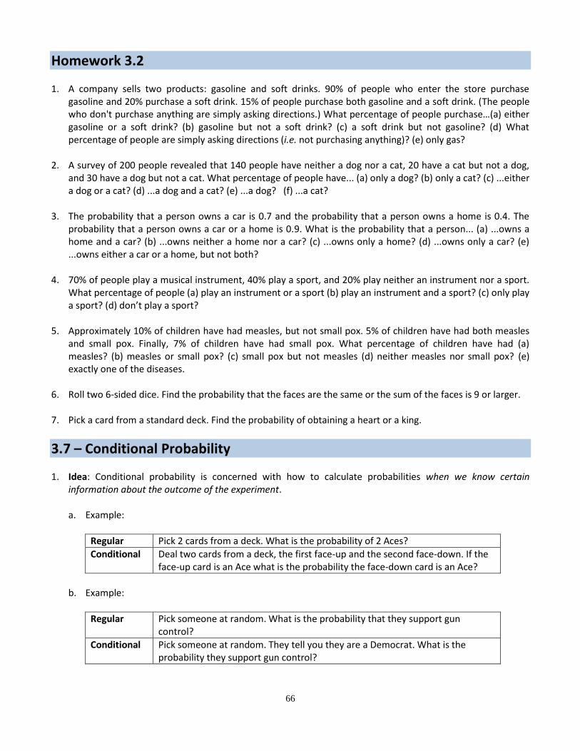
Homework 3.2 1. A company sells two products: gasoline and soft drinks. 90% of people who enter the store purchase
gasoline and 20% purchase a soft drink. 15% of people purchase both gasoline and a soft drink. (The people who don't purchase anything are simply asking directions.) What percentage of people purchase…(a) either gasoline or a soft drink? (b) gasoline but not a soft drink? (c) a soft drink but not gasoline? (d) What percentage of people are simply asking directions (i.e. not purchasing anything)? (e) only gas?
2. A survey of 200 people revealed that 140 people have neither a dog nor a cat, 20 have a cat but not a dog,
and 30 have a dog but not a cat. What percentage of people have... (a) only a dog? (b) only a cat? (c) ...either a dog or a cat? (d) ...a dog and a cat? (e) ...a dog? (f) ...a cat?
3. The probability that a person owns a car is 0.7 and the probability that a person owns a home is 0.4. The
probability that a person owns a car or a home is 0.9. What is the probability that a person... (a) ...owns a home and a car? (b) ...owns neither a home nor a car? (c) ...owns only a home? (d) ...owns only a car? (e) ...owns either a car or a home, but not both?
4. 70% of people play a musical instrument, 40% play a sport, and 20% play neither an instrument nor a sport.
What percentage of people (a) play an instrument or a sport (b) play an instrument and a sport? (c) only play a sport? (d) don’t play a sport?
5. Approximately 10% of children have had measles, but not small pox. 5% of children have had both measles
and small pox. Finally, 7% of children have had small pox. What percentage of children have had (a) measles? (b) measles or small pox? (c) small pox but not measles (d) neither measles nor small pox? (e) exactly one of the diseases.
6. Roll two 6-sided dice. Find the probability that the faces are the same or the sum of the faces is 9 or larger.
7. Pick a card from a standard deck. Find the probability of obtaining a heart or a king.
3.7 – Conditional Probability 1. Idea: Conditional probability is concerned with how to calculate probabilities when we know certain
information about the outcome of the experiment. a. Example:
Regular Pick 2 cards from a deck. What is the probability of 2 Aces?
Conditional Deal two cards from a deck, the first face-up and the second face-down. If the face-up card is an Ace what is the probability the face-down card is an Ace?
b. Example:
Regular Pick someone at random. What is the probability that they support gun control?
Conditional Pick someone at random. They tell you they are a Democrat. What is the probability they support gun control?

67
c. Example:
Regular What is the probability a machine will last 10 years?
Conditional What is the probability a machine will last 10 years given that it has already lasted 4 years?
2. Definition – The conditional probability of event A given event B is:
𝑃(𝐴|𝐵) =𝑃(𝐴 ∩ 𝐵)
𝑃(𝐵)
The phrase given event B means that B is a fact, it has definitely occurred. Using this definition, we can also write:
𝑃(𝐵|𝐴) =𝑃(𝐴 ∩ 𝐵)
𝑃(𝐴)
3. Example: Two types of defects occur on a product. Type A defects occur with probability
0.05, Type B with probability 0.07, and both types of defects occur with probability 0.03. a. Given that a Type B defect occurred, what is the probability that a Type A defect
occurred?
𝑃(𝐴|𝐵) =𝑃(𝐴 ∩ 𝐵)
𝑃(𝐵)=
0.03
0.07= 0.43 = 43%
b. Given that a Type A defect occurred, what is the probability that a Type B defect occurred?
𝑃(𝐵|𝐴) =𝑃(𝐴 ∩ 𝐵)
𝑃(𝐴)=
0.03
0.05= 0.6 = 60%
4. Example: Roll two dice. Given that the sum is 9 or higher, what is the probability that the sum is 10 or
higher? See diagram on page 77 if necessary.
𝑃(𝑠𝑢𝑚 ≥ 10|𝑠𝑢𝑚 ≥ 9) =𝑃(𝑠𝑢𝑚 ≥ 10 ∩ 𝑠𝑢𝑚 ≥ 9)
𝑃(𝑠𝑢𝑚 ≥ 9)=
𝑃(𝑠𝑢𝑚 ≥ 10)
𝑃(𝑠𝑢𝑚 ≥ 9)
=6/36
10/36= 0.6 = 60%
3.7 – Independence 1. Independence – Two events are independent if they are unrelated. In other words, if knowledge of the
outcome of one event in no way influences the probability of the outcome of the other. Mathematically, two events, A and B are independent if:
𝑃(𝐴|𝐵) = 𝑃(𝐴).
2. Example: Using the data from Example 3 above, are Type A and Type B defects independent?
No, because 𝑃(𝐴|𝐵) = 0.43 and 𝑃(𝐴) = 0.05, or because 𝑃(𝐵|𝐴) = 0.6 and 𝑃(𝐵) = 0.07

68
3. Example: Roll two dice, one-at-a-time. Dice rolls (and coin tosses) are independent. It is obvious! If you roll a 6 on the first roll there is no way that can influence the second roll. Suppose you have rolled four 6’s in a row. What is the probability that the 5th roll is a 6? The rolls are independent so the probability is 1/6. The previous 4 sixes don’t influence the 5th roll.
4. Example: Cards are generally not independent. For example, let:
𝐴 = 𝑝𝑖𝑐𝑘 𝑎𝑛 𝑎𝑐𝑒 𝑓𝑟𝑜𝑚 𝑎 𝑑𝑒𝑐𝑘 𝑜𝑓 𝑐𝑎𝑟𝑑𝑠 𝐵 = 𝑝𝑖𝑐𝑘 𝑎𝑛 𝑗𝑎𝑐𝑘 𝑓𝑟𝑜𝑚 𝑎 𝑑𝑒𝑐𝑘 𝑜𝑓 𝑐𝑎𝑟𝑑𝑠
Then: 𝑃(𝐴|𝐵) = 4/51 ≠ 𝑃(𝐴) = 4/52
Note, this is obvious too! If you pick a jack from the deck, of course that will change the probability of obtaining an ace because there is one less card in the deck.
5. If A and B are independent then 𝑃(𝐴 ∩ 𝐵) = 𝑃(𝐴)𝑃(𝐵)
a. Example: Flip two coins. What is the probability of 2 heads?
𝐴 = ℎ𝑒𝑎𝑑 𝑜𝑛 𝑓𝑖𝑟𝑠𝑡 𝑓𝑙𝑖𝑝 𝐵 = ℎ𝑒𝑎𝑑 𝑜𝑛 𝑠𝑒𝑐𝑜𝑛𝑑 𝑓𝑙𝑖𝑝
A and B are independent, so: 𝑃(𝑡𝑤𝑜 ℎ𝑒𝑎𝑑𝑠) = 𝑃(𝐴 ∩ 𝐵) = 𝑃(𝐴)𝑃(𝐵) =1
2∙
1
2=
1
4
b. Example: A batter has a 0.350 batting average. Suppose each time the batter goes to the plate, the
outcome is independent of the others. What is the probability that in the batters next 4 at-bats, he gets first a hit, then another hit, followed by an out, and a hit?
𝑃(𝐻1 ∩ 𝐻2 ∩ �̅�3 ∩ 𝐻4) = 0.35 ∙ 0.35 ∙ (1 − 0.35) ∙ 0.35 = 0.028 Note: this question is different from: What is the probability that the player gets 3 hits in his next 4 at bats.
Homework 3.3 1. A company sells two products: gasoline and soft drinks. 90% of people who enter the store purchase
gasoline and 20% purchase a soft drink. 15% of people purchase both gasoline and a soft drink. (The people who don't purchase anything are simply asking directions.) (a) Suppose that someone purchases gas in the store, what is the probability that they will also purchase a soft drink? (b) Suppose that someone purchases a soft drink in the store, what is the probability that they will also purchase gasoline? (c) Are purchasing gasoline and purchasing a soft drink independent? Why or why not?
2. A survey reveals that 50% of Americans own a home, 20% own a handgun, and 10% own a home and a
handgun. (a) Suppose that someone owns a gun, what is the probability that they also own a home? (b) Are handgun ownership and home ownership independent? Why or why not?
3. 70% of people play a musical instrument, 40% play a sport, and 20% play neither an instrument nor a sport.
(a) Suppose that you see someone playing basketball, what is the probability that they also play a musical instrument? (b) Suppose that you see someone playing a guitar, what is the probability that they also play a

69
sport? (c) Suppose that you see someone playing a guitar, what is the probability that they do not play a sport?
4. Approximately 15% of children have had measles, 7% small pox, and 5% of children have had both measles
and small pox. Are measles and small pox independent? Justify your answer.
5. Pick a card from a standard deck. Suppose someone looks at the card and tells you it is a King, what is the probability that the card is a Heart?
6. Pick a card from a standard deck. Suppose someone looks at the card and tells you it is a Heart, what is the probability that the card is a King?
7. There are 2 kinds of soda in a cooler: 5 Cokes and 10 Diet-Cokes. Also, there are 10 beers in the cooler. A friend picks one can at random and tells you it is a soda. What is the probability that it is a Diet-Coke?
8. Roll a die 3 times. What is the probability that you get a. you get a 1 on first roll, 4 on second, and a 3 on third? b. three 6’s? c. first roll is 3 or more, second roll is 2 or more, and third roll is 3 or less?
3.8 – Two-way Tables 1. A two-way table is essentially the same as Venn diagrams, only we arrange the data in a table as
opposed to the Venn diagram. The “two” refers to the fact that we are dealing with two variables. In the example below, the two variables are:
𝑆𝑒𝑥 ∈ {𝑀𝑎𝑙𝑒, 𝐹𝑒𝑚𝑎𝑙𝑒} 𝑃𝑟𝑜𝑚𝑜𝑡𝑖𝑜𝑛 𝑆𝑡𝑎𝑡𝑢𝑠 ∈ {𝑃𝑟𝑜𝑚𝑜𝑡𝑒𝑑, 𝑁𝑜𝑡 𝑃𝑟𝑜𝑚𝑜𝑡𝑒𝑑}
2. Example: A major metropolitan police force in the eastern U.S. consists of 1200 officers - 960 men
and 240 women. Over the past 2 years, 324 officers on the police force have been awarded promotions. The two-way table below summarizes the breakdown for male and female officers. After reviewing the data, a committee of female officers charged discrimination on the basis that 288 male officers had received promotions, whereas only 36 female officers had received promotions. The police administration countered with the argument that the relatively low number of promotions for female officers was not due to discrimination but due to the fact that there are fewer female officers on the police force.
Male Female Totals
Promoted 288 36 324 Not Promoted 672 204 876
Totals 960 240 1200

70
In analyzing a two-way table, the first thing we do is find the joint and marginal probabilities.
Male Female Totals
Promoted 288
1200= 0.24
36
1200= 0.03
324
1200= 0.27
Not Promoted 672
1200= 0.56
204
1200= 0.17
876
1200= 0.73
Totals 960
1200= 0.8
240
1200= 0.2
Using some notation, we interpret these probabilities as shown below:
Male (𝑴) Female (�̅�) Totals
Promoted (𝑷) 𝑃(𝑀 ∩ 𝑃) 𝑃(�̅� ∩ 𝑃) 𝑃(𝑃) Not Promoted (�̅�) 𝑃(𝑀 ∩ �̅�) 𝑃(�̅� ∩ �̅�) 𝑃(�̅�) Totals 𝑃(𝑀) 𝑃(�̅�)
3. Example – If you pick someone at random from this police force, what is the probability that you
pick...
a. ...a woman? b. ...a man? c. ...someone who was promoted? d. ...a person who was not promoted? e. ...a man who was promoted? f. ...a man who was not promoted? g. ...a woman who was promoted?
h. ...a woman who was not promoted? i. ...someone who was promoted or a
woman? j. ...someone who was not promoted or a
woman? k. ...someone who was promoted or a man? l. ...someone who was not promoted or a
man?

71
Suppose you pick someone at random from the police force and discover that they...
m. ...are a woman, what is the probability that she was promoted? n. ...are a woman, what is the probability that she was not promoted? o. ...are a man, what is the probability that he was promoted? p. ...are a man, what is the probability that he was not promoted? q. Are promotion status and sex independent? Why?
Homework 3.4 1. The data shown on the right was collected about voter preference for
males and females. Each person in the survey was asked whether they would vote for McCain or Obama, and their sex was noted. Suppose that you pick someone at random, what is the probability that the person…
a. ...votes for McCain? b. ...is a female that votes for
Obama? c. …is a male who didn’t vote for
McCain? d. …is a female? e. …is a female or voted for Obama?
f. Suppose that you pick a person at random and observe that they are a female, what is the probability that the person voted for Obama?
g. Suppose that you pick a person at random and discover that they voted for McCain, then what is the probability that the person is a Male?
h. Are voter’s preference and sex independent? Why or why not?
2. A survey of 207 college students is conducted to find the numbers of students that have cell phones and
cars. The survey reveals that 42 have a car and a cell phone; 126 have a car but not a cell phone; 28 do not have a car but do have a cell phone; and 11 have neither a car nor a cell phone.
a. Make a two-way table to represent this data.
Suppose you pick someone at random, what is the probability that the person... b. ...has a cell phone? c. ...has a car? d. ...does not have a cell phone? e. ...has a cell phone and a car? f. ...has a cell phone but not a car? g. ...does not have a car or a cell
phone?
Suppose that you pick someone at random and the person tells you they… h. have a car. What is the probability that they have a cell
phone? i. have a cell phone. What is the probability that they
have a car? j. do not have a car. What is the probability that they
have a cell phone? k. do not have a car. What is the probability that they do
not have a cell phone? l. Are owning a car and having a cell phone
independent? Why?
Male Female
McCain 420 140 Obama 490 350

72
Chapter 4 – Discrete Probability Distributions In this chapter we get slightly more formal about probability.
4.1 – Random Variables 1. Random Variable (RV) – A random variable is a numerical description of the outcome of an experiment. 2. Example – When we flip two coins, the sample space is: {𝑇𝑇, 𝑇𝐻, 𝐻𝑇, 𝐻𝐻}.
Suppose we let 𝑋 = 𝑡ℎ𝑒 𝑛𝑢𝑚𝑏𝑒𝑟 𝑜𝑓 𝐻𝑒𝑎𝑑𝑠 𝑖𝑛 𝑡𝑤𝑜 𝑓𝑙𝑖𝑝𝑠 𝑜𝑓 𝑎 𝑐𝑜𝑖𝑛. X is called a discrete random variable and takes on the values {0, 1, 2}. Note that X is a numerical description of the outcome of this experiment, it counts the number of Heads in two coin tosses. Thus:
𝑃(𝑋 = 0) = 𝑃(𝑇𝑇) =1
4.
𝑃(𝑋 = 1) = 𝑃(𝑇𝐻 𝑜𝑟 𝐻𝑇) =1
4+
1
4=
1
2.
𝑃(𝑋 = 2) = 𝑃(𝐻𝐻) =1
4.
Notice that these three probabilities add up to 1.
7. Example –Let 𝑋 = 𝑛𝑢𝑚𝑏𝑒𝑟 𝑜𝑓 ℎ𝑒𝑎𝑑𝑠 𝑖𝑛 4 𝑐𝑜𝑖𝑛 𝑡𝑜𝑠𝑠𝑒𝑠
𝑋 ∈ {0,1,2,3,4} What are the probabilities of each of the values the random variable can take on?

73
3. Discrete Random Variable – A discrete RV takes on a finite number of values. Thus, we can count all the values, there is separation between the values. Many times, a discrete random variable is a count of something. Examples:
Let X = the number of defects on a product, X can be: {0, 1, 2, …}
Let X = the number of boxes of cereal out of 50 that have more than 5 fat grams per serving. Thus, X can be {0, 1, 2, …, 49, 50}
Let X = the sum of the faces of two dice that are rolled. Thus, X can be {2, 3, 4, …, 10, 11, 12}
Let X = the number of accidents at an intersection in an hour. Thus, X can be {0, 1, 2, …}
4. Continuous Random Variable – A continuous RV can take on ALL values in a given interval. Many times, a continuous random variable is a scientific measurement. We will study these in Chapter 6. Examples:
Let X = lifetime of a light bulb. Thus, X might take on any value in [1 hour, 5000 hours]
Let X = the height of a plant. Thus, X might take on any value in [6in, 18in]
Let X = the weight of a person. Thus, X might take on any value in [90 lbs, 400 lbs]
Let X = the time between successive accidents. Thus, X might take on any value in [0min, 3000 min]
Let X = the fat grams in a serving of cereal. Thus, X might take on any value in [2.5 gms, 4.5 gms.]
Let X = the gas mileage of a car. Thus, X might take on any value in [24 mpg, 33 mpg]
4.2 – Calculating Discrete Probabilities 1. Discrete Probability Function, 𝑓(𝑥) – provides the probabilities of all the values a random variable can take
on. For a discrete RV, the probability that X takes on a particular value is simply the function evaluated at that value:
𝑃(𝑋 = 𝑐) = 𝑓(𝑐)
2. Example – Suppose we have a probability function, 𝑓(𝑥) =𝑥
6, 𝑥 = 1,2,3. This tells us that the discrete
random variable takes on exactly the value 1,2, or 3 and that:
𝑃(𝑋 = 1) = 𝑓(1) = 1/6 𝑃(𝑋 = 2) = 𝑓(2) = 2/6 𝑃(𝑋 = 3) = 𝑓(3) = 3/6
3. Properties of a discrete probability function:
1. 0 ≤ 𝑓(𝑥) ≤ 1, as we said earlier, probabilities are always between 0 and 1.
2. ∑ 𝑓(𝑥) = 1, as we said earlier, all the probabilities in the sample space must add to 1. 4. Probability functions are given in a table, graph, mathematical formula, or in words.
Example – Note that the four examples below all convey the same probability function.
1. Formula 𝑓(𝑥) =
𝑥
6, 𝑥 = 1,2,3

74
2. Table x )(xf
1 1/6
2 1/3
3 1/2
3. Graph
4. Words A random variable takes on values 1, 2, and 3 with probabilities
1/6, 1/3, and 1/2, respectively. 5. Important Rules for Calculating Probabilities for Discrete Random Variables.
Example: 𝑓(𝑥) =𝑥
42, 𝑥 = 2, 4, 6, 8, 10, 12
a. 𝑃(𝑋 = 𝑐) = 𝑓(𝑐)
𝑃(𝑋 = 8) = 𝑓(8) = 8/42
b. 𝑃(𝑋 ≤ 𝑐) =∑ 𝑓(𝑥)𝑥 ≤ 𝑐
𝑃(𝑋 ≤ 8) = 𝑓(2) + 𝑓(4) + 𝑓(6) + 𝑓(8) =2
42+
4
42+
6
42+
8
42= 20/42
c. 𝑃(𝑋 < 𝑐) =∑ 𝑓(𝑥)𝑥 < 𝑐
𝑃(𝑋 < 8) = 𝑓(2) + 𝑓(4) + 𝑓(6) =2
42+
4
42+
6
42= 12/42
Note: 𝑃(𝑋 < 8) = 𝑃(𝑋 ≤ 6) for this particular problem.
d. 𝑃(𝑋 ≥ 𝑐) =∑ 𝑓(𝑥)𝑥 ≥ 𝑐
= 1 − 𝑃(𝑋 < 𝑐)
𝑃(𝑋 ≥ 8) = 𝑓(8) + 𝑓(10) + 𝑓(12) =8
42+
10
42+
12
42= 30/42
or
𝑃(𝑋 ≥ 8) = 1 − 𝑃(𝑋 < 8) = 1 − [𝑓(2) + 𝑓(4) + 𝑓(6)] = 1 −12
42= 30/42
e. 𝑃(𝑋 > 𝑐) =∑ 𝑓(𝑥)𝑥 > 𝑐
= 1 − 𝑃(𝑋 ≤ 𝑐)
1/6
1
2/6
23
3/6
x
f(x)

75
𝑃(𝑋 > 8) = 𝑓(10) + 𝑓(12) =10
42+
12
42= 22/42
Or
𝑃(𝑋 > 8) = 1 − 𝑃(𝑋 ≤ 8) = 1 − [𝑓(2) + 𝑓(4) + 𝑓(6) + 𝑓(8)] =
1 −20
42= 22/42
f. 𝑃(𝑎 ≤ 𝑋 ≤ 𝑏) = 𝑃(𝑋 ≤ 𝑏) − 𝑃(𝑋 < 𝑎)
𝑃(6 ≤ 𝑋 ≤ 10) = 𝑃(𝑋 ≤ 10) − 𝑃(𝑋 < 6) = 𝑃(𝑋 ≤ 10) − 𝑃(𝑋 ≤ 4)
𝑃(𝑋 ≤ 10) = 𝑓(2) + 𝑓(4) + 𝑓(6) + 𝑓(8) + 𝑓(10) = 30/42
𝑃(𝑋 ≤ 4) = 𝑓(2) + 𝑓(4) = 6/42
=30
42−
6
42= 24/42
or
𝑃(6 ≤ 𝑋 ≤ 10) = 𝑓(6) + 𝑓(8) + 𝑓(10) = 24/42
6. Example 1 – Given the probability function shown in the table below, find the probability that X is
a. 6 or less. b. less than 6. c. 5 or 7. d. not 6.
𝑥 𝑓(𝑥) 4 0.2
5 0.2
6 0.3
7 0.3
7. Example 2 – A probability function is: (𝒙) = |𝒙−𝟑|
𝟏𝟓, 𝒙 = −𝟐, −𝟏, 𝟎, 𝟏, 𝟐 . Find the probability that X is ...
a. -2 b. 2 c. 0 d. negative e. between -1 and 1, inclusive
8. Example 2 – A probability function is: (𝒙) = 𝒙
𝟓𝟎𝟓𝟎, 𝒙 = 𝟏, 𝟐, … , 𝟏𝟎𝟎 . Find the probability that X is ...
a. at most 3. Thus, 𝑃(𝑋 ≤ 3) =?. Note:
𝑃(𝑋 ≤ 3) = 𝑓(1) + 𝑓(2) + 𝑓(3) =1
5050+
2
5050+
3
5050=
6
5050= 0.0012
b. at least 4. Thus, 𝑃(𝑋 ≥ 4) =? Note:
Thus, 𝑃(𝑋 ≤ 3) + 𝑃(𝑋 ≥ 4) = 1 ⟹ 𝑃(𝑋 ≥ 4) = 1 − 𝑃(𝑋 ≤ 3)

76
So, 𝑃(𝑋 ≥ 4) = 1 −6
5050=
5044
5050= 0.9988
c. 98 or less. Note:
So, 𝑃(𝑋 ≤ 98) = 1 − 𝑃(𝑋 ≥ 99) = 1 − [𝑓(99) + 𝑓(100)]
= 1 − (99
5050+
100
5050) = 1 −
199
5050=
4851
5050= 0.9606
d. greater than 2. Note:
So, 𝑃(𝑋 > 2) = 1 − 𝑃(𝑋 ≤ 2) = 1 − [𝑓(1) + 𝑓(2)]
= 1 − (1
5050+
2
5050) = 1 −
3
5050=
5047
5050= 0.9994
9. Example 4 – Suppose that X has probability function, 𝒇(𝒙) = 𝒄𝒙, 𝒙 = 𝟐, 𝟒, 𝟔, where c is a constant. Find the
value of c. Remember that: ∑ 𝑓(𝑥) = 1
∑ 𝑓(𝑥) = 2𝑐 + 4𝑐 + 6𝑐 = 12𝑐 = 1 ⇒ 𝑐 = 1/12
Thus, 𝑓(𝑥) =𝑥
12, 𝑥 = 2,4,6 is a valid probability function.
10. Example 4 – Suppose that X has probability function, 𝒇(𝒙) =𝒙−𝟏𝟎
𝒄, 𝒙 = 𝟐𝟎, 𝟑𝟎, 𝟒𝟎 where c is a constant.
Find the value of c.
∑ 𝑓(𝑥) = 20−10
𝑐+ 30−10
𝑐+ 40−10
𝑐= 60
𝑐= 1 ⇒ 𝑐 = 60
Thus, 𝑓(𝑥) =𝑥−10
60, 𝑥 = 20,30,40, is a valid probability function.
Homework 4.1 Consider the following probability function for the next six questions.
𝑓(𝑥) =11 − 𝑥
55, 𝑥 = 1, 2, … , 9, 10
Find the probability that X is ...
1. ...exactly 8. (a) 0.8 (b) 0.1 (c) 0.054 (d) 0.11 (e) 0.89

77
2. ...less than 4. (a) 0.49 (b) 0.75 (c) 0.6 (d) 0.7 (e) 0.3 3. ...3 or greater. (a) 0.8 (b) 0.65 (c) 0.3 (d) 0.33 (e) 0.75 (f) 0.67
4. ...not 5. (a) 0.65 (b) 0.5 (c) 0.33 (d) 0.67 (e) 0.89 (f) 0.94
5. ...more than 8. 6. ...at least 6 but no more than 8.
Consider the following probability function for the next four questions.
𝑓(𝑥) =|𝑥|
12, 𝑥 = −4, −2, 2, 4
Find the probability that X is ... 7. ...-2. 8. ...negative. 9. …positive 10. …either 2 or -2
11. Consider this probability function, 𝑓(𝑥) =𝑥2
𝑐, 𝑥 = 1,2,3, where c is a constant. Find the value of c that
makes this a probability function. 12. Consider this probability function, 𝑓(𝑥) = 𝑐𝑥3, 𝑥 = 1,2,3, where c is a constant. Find the value of c that
makes this a probability function.
4.3 – Expected Value 1. Expected Value of X (of a discrete RV) – The expected value of a random variable is the long-run average
value of a random variable. It is what we expect to happen, on average in the long-run. It is a measure of the center of X. It is also called the mean of the RV X.
2. We use the symbol 𝐸[𝑋] or 𝜇 to denote the expected value of a random variable. It is computed by taking each value and multiplying by the respective probability, then adding these products:
𝜇 = 𝐸[𝑋] = ∑ 𝑥𝑓(𝑥)
𝑎𝑙𝑙 𝑥
3. Example – Consider the probability function: 𝑓(𝑥) =𝑥
6, 𝑥 = 1, 2, 3. Find the expected value of the random
variable, X.
𝜇 = 𝐸[𝑋] = ∑ 𝑥𝑓(𝑥)
𝑎𝑙𝑙 𝑥
= 1 (1
6) + 2 (
2
6) + 3 (
3
6) =
7
3= 2.33

78
1/6
1
2/6
23
3/6
x
f(x)Does this answer make sense? The idea is that there is an experiment that results in an outcome of 1, 2, or 3. Do this experiment many times and then compute the sample average of all the outcomes. What do we expect the answer to be? Look at the graph below. Most of the time you do the experiment, you get a "3", sometimes you get a "2", and occasionally you get a "1". So, it should make sense that the long-run average value from doing this experiment is between 2 and 3, i.e. 2.33.
4. Example –Suppose you have the opportunity to play the following game
as frequently as you like. You win $10 with probability 0.4 and lose $5 with probability 0.6. Ignore the cost of playing the game (assume that is factored into the payoff). Would you want to play this game once? A few times? Never? As frequently as possible?
Solution:
x f(x)
$10 0.4
-$5 0.6
𝜇 = 𝐸[𝑋] = ∑ 𝑥𝑓(𝑥) = $10(0.4) + (−$5)(0.6) = $4 + (−$3) = $1
The expected value of this game is $1. What does this number mean? It means that if I am going to play this game many times, on average I will win $1. So, I want to play the game as frequently as possible! If I play the game 1000 times, I would win approximately $1000. If I play the game a few times, I'm not sure what will happen. Another way to think about this is as follows. If I agree to play the game many times, we don't have to play the game at all! Every time I want to play, I'll tell you, and you can give me $1. The result will be the same in the long-run, the same as if we had played the game!
5. Example – Consider the following probability function, 𝑓(𝑥) =|𝑥−3|
15, 𝑥 = −2, −1,0,1,2. Find the mean of
X.
𝜇 = 𝐸[𝑋] = ∑ 𝑥𝑓(𝑥) = −2 (5
15) + (−1) (
4
15) + 0 (
3
15) + 1 (
2
15) + 2 (
1
15) =
−10
15= −
2
3= −0.667
6. Example – What is the expected value of a single roll of a die.
𝜇 = 𝐸[𝑋] = ∑ 𝑥𝑓(𝑥) = 1 (1
6) + 2 (
1
6) + 3 (
1
6) + 4 (
1
6) + 5 (
1
6) + 6 (
1
6) =
21
6= 3.5
4.4 – Variance
1. Variance of X – The variance of a random variable is a measure of how spread out the values of X are.
2. We use the symbol 𝑉[𝑋] or 𝜎2 to denote the variance of a random variable. The definition is:
𝜎2 = 𝑉[𝑋] = ∑(𝑥 − 𝜇)2𝑓(𝑥)
However, a simpler formula for computing is:

79
𝜎2 = 𝑉[𝑋] = 𝐸[𝑋2] − 𝜇2
Where:
𝐸[𝑋2] = ∑ 𝑥2𝑓(𝑥) 3. Standard Deviation of X – The standard deviation of a random variable is the square-root of the variance:
𝜎 = √𝜎2. Usually, we are interested in the standard deviation as opposed to the variance because it has units which are the same as the units of the variable.
4. To calculate the standard deviation we use these steps:
1. 1. Find the expected value of 𝑋: 𝜇 = 𝐸[𝑋] = ∑ 𝑥𝑓(𝑥)
2. 2. Find the expected value of 𝑋2: 𝐸[𝑋2] = ∑ 𝑥2𝑓(𝑥)
3. 3. Find the variance of 𝑋: 𝜎2 = 𝑉[𝑋] = 𝐸[𝑋2] − 𝜇2
4. 4. Find the standard deviation of 𝑋: 𝜎 = √𝜎2
5. Example: Consider the probability function: 3,2,1,6
)( xx
xf . Find the variance and standard
deviation of the random variable, X.
a. 33.23
7
6
33
6
22
6
11)(][
xxfXE
b. 66
33
6
22
6
11)(][ 22222
xfxXE
c. 556.09/53
76][][
2
222
XEXV
d. 745.09
5 2 =
6. Example: Same as Example 4 in the previous section (You win $10 with probability 0.4 and lose $5 with
probability 0.6). Find the variance and standard deviation of the payoff from this game.
a. 1$)3$(4$6.0)5$(4.010$)(][ xxfXE
b. 556.0)5$(4.0)10($)(][ 2222 xfxXE
c. 54155][][2222 XEXV
d. 348.7$54 2 =

80
7. Example: Consider the following probability function, 𝑓(𝑥) =|𝑥−3|
15, 𝑥 = −2, −1,0,1,2. Find the variance
and standard deviation of X.
a. 𝜇 = −2
3= −0.667 (from a previous example)
b. 𝐸[𝑋2] = ∑ 𝑥2𝑓(𝑥) = (−2)2 (5
15) + (−1)2 (
4
15) + 02 (
3
15) + 12 (
2
15) + 22 (
1
15) =
30
15= 2
c. 𝜎2 = 𝑉[𝑋] = 𝐸[𝑋2] − 𝜇2 = 2 − (−2
3)
2=
14
9= 1.555
d. 𝜎 = √𝑉[𝑋] = √14
9=
√14
3= 1.247
8. Comparing Investments – Investment opportunities are frequently compared by answering these questions:
1. What is expected return? We answer this by interpretting the expected value,
2. How much volatility is there? We answer this by interpretting the standard deviation, 3. What is the probability that we will return a profit?
9. Example: Investment A pays $100 with probability 1/10, $500 with probability 3/5, and -$100 with probability 3/10. Investment B pays $300 with probability 2/5, $400 with probability 2/5, and -$50 with probability 1/5. Which investment do you prefer and why?
Investment A Investment B
𝑥 𝑓(𝑥) 𝑥 𝑓(𝑥)
$100 1/10 $300 2/5
$500 3/5 $400 2/5
-$100 3/10 -$50 1/5
Criteria
Investment A Investment B
𝜇𝐴 = $280 𝜇𝐵 = $270 𝜎𝐴 = $275 𝜎𝐵 = $166 𝑃(𝐴 𝑟𝑒𝑡𝑢𝑟𝑛𝑠 𝑎 𝑝𝑟𝑜𝑓𝑖𝑡) = 0.7 𝑃(𝐵 𝑟𝑒𝑡𝑢𝑟𝑛𝑠 𝑎 𝑝𝑟𝑜𝑓𝑖𝑡) = 0.8
Summary: The answer to the problem is, it depends:
1. If you are going to invest many times, you probably only need to look at the expected return, in which
case you choose Investment A.
2. If you are going to invest a few times, you juggle the expected return and the volatility. How you do this depends on your tolerance for risk. In other words, if your tolerance for risk is low, you may choose an investment with a lower expected return because it has less volatility. For this problem, Investment B has less risk, 𝜎𝐵 = $166 < $275 = 𝜎𝐴, but a smaller expected return, 𝜇𝐵 = $270 < $280 = 𝜇𝐴.
3. If you are going to invest one time, you might also want to take into account the probability that the investment will return a profit. For this problem, Investment B has a 10% higher chance of returning a profit.

81
Homework 4.2 Consider the following probability function for the next two questions:
𝑥 3 4 5
𝑓(𝑥) 0.7 0.2 0.1 1. The expected value of the random variable X is: (a) 4 (b) 3.4 (c) 1.6 (d) 12 (e) 0.33 2. The standard deviation of the random variable X is: (a) 16.67 (b) 12 (c) 19.22 (d) 11.56 (e) 0.66 (f) 3.47
Consider the following probability function, 6,4,2,12
)( xx
xf .
3. Find the mean of the random variable X. 4. Find the variance of the random variable X. 5. Find the standard deviation of the random variable X. Consider an investment that returns $5 with probability 0.4, $2 with probability 0.2, and -$9 with probability 0.4. 6. What is the expected return of this investment? 7. Is this a good investment for the long-run? Why or why not? 8. What is the volatility of this investment?
4.5 – Binomial Distribution 1. Binomial Distribution –
The binomial distribution is a special probability function. This is because it explains a pattern that occurs in some real problems.
We use the notation, 𝑋~𝐵𝑖𝑛(𝑛, 𝑝) to say that the random variable X follows (or has) the binomial distribution.
n and p are called the parameters of the distribution. This means that we must know the values of n and p before we can do any calculations.
The probability function for a binomial random variable is:
𝑓(𝑥) = (𝑛𝑥
) 𝑝𝑥(1 − 𝑝)𝑛−𝑥 , 𝑥 = 0, 1, … , 𝑛
=𝑛!
𝑥!(𝑛−𝑥)!𝑝𝑥(1 − 𝑝)𝑛−𝑥
We will not need this formula because our calculator will calculate it for us.
Mean and Variance of Binomial RV – Since the binomial distribution follows a pattern, it can be shown that the expected value of a Binomial random variable is: 𝜇 = 𝑛𝑝 and the variance is: 𝜎2 = 𝑛𝑝(1 − 𝑝).

82
0.00
0.05
0.10
0.15
0.20
0.25
0.30
0.35
0.40
0 1 2 3 4 5
Pro
bab
ility
x
2. Example – Suppose a baseball player goes to bat 5 times in a game and that his batting average is 0.333. Find the probability distribution for the number of hits in five at-bats assuming that each time at the plate is independent of the others.
Let X = number of hits in 5 at-bats, 𝑋 ∈ {0,1,2,3,4,5}
This problem can be answered with the binomial distribution (we will show why later) and we can write:
𝑋~𝐵𝑖𝑛(𝑛 = 5, 𝑝 = 0.333)
This is a graph of the probabilities is shown on the right.
3. Example – A drug works 90% of the time in curing an
infection. A sample of 100 people with the infection is chosen and each is given the drug. Find the probability distribution for the number of people who are cured.
Let X = number of people cured out of 100, 𝑋 ∈{0,1, … , 100}
This problem can also be answered with the binomial distribution and we can write:
𝑋~𝐵𝑖𝑛(𝑛 = 100, 𝑝 = 0.9)
These are some graphs of the probabilities:
90% Success Rate 50% Success Rate
90% Success Rate 50% Success Rate
0.00
0.02
0.04
0.06
0.08
0.10
0.12
0.14
0 20 40 60 80 100
Pro
bab
ility
x
0.00
0.02
0.04
0.06
0.08
0.10
0.12
0.14
0 10 20 30 40 50 60 70 80 90 100
Pro
bab
ility
x
0.00
0.02
0.04
0.06
0.08
0.10
0.12
0.14
75 80 85 90 95 100
Pro
bab
ility
x
0.00
0.02
0.04
0.06
0.08
30 40 50 60 70
Pro
bab
ility
x

83
What is the mean number of people who are cured? Another way to ask this is, What is the expected number of people who will be cured?
𝜇 = 𝑛𝑝 = 100 ∗ 0.9 = 90 people 𝜇 = 𝑛𝑝 = 100 ∗ 0.5 = 50
What is the variance and standard deviation of the number of people who are cured?
𝜎2 = 𝑛𝑝(1 − 𝑝) = 100 ∗ 0.9 ∗ (1 − 0.9) = 9
𝜎 = √𝜎2 = √9 = 3 people.
𝜎2 = 𝑛𝑝(1 − 𝑝) = 100 ∗ 0.5 ∗ (1 − 0.5) = 25
𝜎 = √𝜎2 = √25 = 5 people.
4. TI 83/84 Binomial Distribution Directions
For the following directions, we assume we know that 𝑋~𝐵𝑖𝑛(𝑛, 𝑝) and that we know the values of n and p. a. We can answer this question: 𝑃(𝑋 = 𝑥) by following these directions:
1. Choose DISTR by pressing 2nd and the VARS key.
2. Scroll down to A:binompdf( and press Enter.
3. Type in: n, p, x and press Enter. Thus, 𝑃(𝑋 = 𝑥) = 𝑏𝑖𝑛𝑜𝑚𝑝𝑑𝑓(𝑛, 𝑝, 𝑥)
b. We can answer this question: 𝑃(𝑋 ≤ 𝑥) by using : “B:binomcdf” (in step 2 above). Thus, 𝑃(𝑋 ≤ 𝑥) = 𝑏𝑖𝑛𝑜𝑚𝑐𝑑𝑓(𝑛, 𝑝, 𝑥)
Any other probability questions will require using simple probability rules to rearrange the question to conform to b immediately above.
c. 𝑃(𝑋 < 𝑥) = 𝑏𝑖𝑛𝑜𝑚𝑐𝑑𝑓(𝑛, 𝑝, 𝑥 − 1)
d. 𝑃(𝑋 ≥ 𝑥) = 1 − 𝑏𝑖𝑛𝑜𝑚𝑐𝑑𝑓(𝑛, 𝑝, 𝑥 − 1)
e. 𝑃(𝑋 > 𝑥) = 1 − 𝑏𝑖𝑛𝑜𝑚𝑐𝑑𝑓(𝑛, 𝑝, 𝑥)
f. 𝑃(𝑎 ≤ 𝑋 ≤ 𝑏) = 𝑏𝑖𝑛𝑜𝑚𝑐𝑑𝑓(𝑛, 𝑝, 𝑏) − 𝑏𝑖𝑛𝑜𝑚𝑐𝑑𝑓(𝑛, 𝑝, 𝑎 − 1)

84
5. Example – Suppose a baseball player goes to bat 5 times in a game and that his batting average is 0.333. What is the probability of getting 3 hits? 3 or fewer hits? 3 or more hits? more than 3 hits? between 2 and 4 hits, inclusive?
As we saw previously:
Let X = number of hits in 5 at-bats, 𝑋 ∈ {0,1,2,3,4,5}
𝑋~𝐵𝑖𝑛(𝑛 = 5, 𝑝 = 0.333)
Thus,
𝑃(𝑋 = 3) = 𝑏𝑖𝑛𝑜𝑚𝑝𝑑𝑓(5,0.333,3) = 0.1643 = 0.16 𝑃(𝑋 ≤ 3) = 𝑏𝑖𝑛𝑜𝑚𝑐𝑑𝑓(5,0.333,3) = 0.9549 = 0.95 𝑃(𝑋 ≥ 3) = 1 − 𝑏𝑖𝑛𝑜𝑚𝑐𝑑𝑓(5,0.333,2) = 0.2094 = 0.21 𝑃(𝑋 > 3) = 1 − 𝑏𝑖𝑛𝑜𝑚𝑐𝑑𝑓(5,0.333,3) = 0.0451 = 0.04 𝑃(2 ≤ 𝑋 ≤ 4) = 𝑏𝑖𝑛𝑜𝑚𝑐𝑑𝑓(5,0.333,4) − 𝑏𝑖𝑛𝑜𝑚𝑐𝑑𝑓(5,0.333,1) = 0.5343 = 0.53
6. When can we use the Binomial distribution? We can use the binomial distribution when three conditions
have been met:
1. Experiment is a sequence of n independent trials. 2. Each trial results in one of two possible outcomes, Success or Failure. Success is defined as what you are
interested in. 3. The probability of Success on each trial is p and is constant from trial to trial.
If the three conditions are met, then the random variable,
X = the number of Successes in n trials.
Follows the binomial distribution with parameters n and p:
𝑋~𝐵𝑖𝑛(𝑛, 𝑝) 7. Example – Roll six dice. What is the probability of obtaining exactly two "4's"? Have the conditions for the
Binomial distribution been met?
1. Experiment is a sequence of n independent trials. We can think of rolling the dice one-at-a-time, thus we have six trials (where a trial is a roll of a single die) and we say that n = 6. Are the trials independent? Yes, the outcome of the first roll in no way influences the outcome of the second roll, etc. So, the first condition has been met.
2. Each trial results in one of two possible outcomes, Success or Failure. Success for this problem is when we roll a die and obtain a "4" and a Failure is anything else. So, we can classify the outcome of each of the six trials (roll of the die) as a Success or a Failure. For instance if I roll: 3, 6, 4, 2, 5, 3, I can classify these as: Failure, Failure, Success, Failure, Failure, Failure. Thus, the second condition has been met.

85
3. The probability of Success on each trial is p and is constant from trial to trial. The probability of Success for this problem is the probability of rolling a single die and obtaining a "4." This probability is known to be 1/6, thus p = P(Success) = P(roll a 4) = 1/6. Is p constant from trial to trial (roll to roll). Yes, the probability of rolling a "4" never changes. Thus, the third condition has been met.
Thus, we see that the three conditions have been met. So,
Let X = the number of "4's" obtained in six rolls of the die. And we say that X has a Binomial distribution with parameters n=6 and p=1/6.
𝑋~𝐵𝑖𝑛(𝑛 = 6, 𝑝 = 1/6) We can also see that the values that X can take on are:
{0,1,2,3,4,5,6} and the question being asked is
𝑃(𝑋 = 2) =? (Answer: 0.2009).
8. Example – A drug is successful 90% of the time in curing a particular disease. The drug is given to a group of 10 people with the disease. Find the probability that eight people are cured.
1. Experiment is a sequence of n independent trials. We can think of giving the drug to the 10 people one-
at-a-time, thus we have ten trials (where a trial is when we give the drug to a single person) and we say that n = 10. Are the trials independent? Yes, whether the drug works on the first person in no way influences whether the drug works on the second person, etc. So, the first condition has been met.
2. Each trial results in one of two possible outcomes, Success or Failure. Success for this problem is when someone is cured and a Failure is when the person is not cured. So, we can classify the outcome of each of the ten trials as a Success or a Failure. Thus, the second condition has been met.
3. The probability of Success on each trial is p and is constant from trial to trial. The probability of Success for this problem is the probability that a person is cured after they take the drug. We assume that this probability is 0.9 since we are told that 90% of people are cured with the drug., thus p = P(Success) = P(a person is cured) = 0.9. Is p constant from trial to trial (person to person). Technically, no. Everybody is different. However, in a situation like this we frequently assume that it is constant for all people.
Thus, we see that the three conditions have been met. So,
Let X = the number of people who are cured out of ten. And we say that X has a Binomial distribution with parameters n=10 and p=0.9.
𝑋~𝐵𝑖𝑛(𝑛 = 10, 𝑝 = 0.9) We can also see that the values that X can take on are:
{0,1,2,3,4,5,6,7,8,9,10}

86
and the question being asked is
𝑃(𝑋 = 8) =? (Answer: 0.1937).
9. Example – Choose 5 cards from a deck. Find the probability of choosing exactly two aces.
1. Experiment is a sequence of n independent trials. We can think of drawing the cards one-at-a-time, thus we have five trials (where a trial is a single card being drawn) and we say that n = 5. Are the trials independent? No, see condition 3 below.
2. Each trial results in one of two possible outcomes, Success or Failure. Success for this problem is when an Ace is drawn and a Failure is when any other card is drawn. So, we can classify the outcome of each of the five trials as a Success or a Failure. Thus, the second condition has been met.
3. The probability of Success on each trial is p and is constant from trial to trial. The probability of Success for this problem is the probability that an Ace is drawn. Note this probability is not constant from draw-to-draw. Why? What is the probability of an Ace on the first draw? The second draw?
This problem does not fit the binomial pattern.
10. Example – A drug is successful 90% of the time in curing a particular disease. In a study of the drug’s effectiveness, a group of 10 people with the disease are given the drug. Assume that the people are independent.
As we saw before, X = the number of people who are cured and 𝑋~𝐵𝑖𝑛(𝑛 = 10, 𝑝 = 0.9). What is the probability that...
a. ...8 people are cured? )8(XP
b. ...8 or fewer people are cured? )8(XP
c. ...less than 8 people are cured? )7()8( XPXP
d. ...at least 7 are cured? 1)6(1)7( XPXP
e. ...more than 7 are cured? 1)7(1)8()7( XPXPXP
f. What is the mean number of people who are cured? g. What is the variance and standard deviation of the number of people who get well? h. ...3 people are not cured?
We can answer this question rather simply by noting that if 3 people are not cured then 7 people are cured: 𝑃(𝑋 = 7) = However, a better approach, especially for the following problems that are a little more tricky is to Let Y = the number of people who are not cured and𝑌~𝐵𝑖𝑛(𝑛 = 10, 𝑝 = 0.1). Then, we can answer the question with: 𝑃(𝑌 = 3) =
i. ...that more than 2 people are not cured? 1)2(1)3()2( YPYPYP
j. What is the mean number of people who are not cured? k. What is the variance of the number of people who are not cured?

87
11. Example – Suppose that a company places orders with a manufacturer frequently. Consider the table below
that shows the number of days it takes to receive an order and the respective probability. An order is considered Late if it is received on the third or fourth day. Assume that orders are independent of one another.
Day 1 2 3 4
Probability 0.20 0.65 0.10 0.05
a. Out of the next ten orders, what is the probability of three or fewer late orders?
Let X = the number of late orders out of the next 10, and )15.005.01.0,10(~ pnBinX .
)3(XP
b. Out of the next 200 orders, how many do we expect to be late?
Let X = the number of late orders out of the next 200, and )15.0,200(~ pnBinX .
Homework 4.3 Consider the following information for the next three questions. A company has purchased many computers from the same supplier over several years and has found that 95% of the computers operate properly upon initial configuration and 5% do not operate properly. Assume the computers are independent of one another.
1. Consider the next shipment of 6 computers to the company. Suppose you want to find the probability that
there are exactly two computers that do not operate properly. (a) Identify the values of n and p and write the probability question. (b) Find the answer using your calculator.
2. Consider the next shipment of 20 computers to the company. Suppose you want to find the probability that
there are at least 17 computers that operate properly. (a) Identify the values of n and p and write the probability question. (b) Find the answer using your calculator.
3. Suppose that over the course of the next year the company plans to purchase 250 computers. How many
computers should the company expect to have problems with?
(a) 5 (b) 10 (c) 11.875 (d) 12.5 (e) 13.825 (f) 21
4. A simple random sample survey in New York City revealed that 15% of city residents use a car as their primary means of transportation, 5% use a motorcycle, 60% use public transportation, 15% use taxis, and the rest walk. Suppose you take a sample of 60 NYC residents and want to find the probability that more than twenty people say they use either a car or a taxi. (a) Identify the values of n and p and write the probability question. (b) Find the answer using your calculator.
5. A baseball player has a batting average of 0.375 and each time he goes to bat is independent of other at
bats. (a) Suppose you want to calculate the probability that the player gets 4 hits in his next 4 at-bats. (a) Identify the values of n and p and write the probability question. (b) Find the answer using your calculator. (c) What about no hits in his next 4 at-bats? (d) Suppose this player goes to bat exactly 4 times in each of 162 games. In how many games do we expect the player to go hitless?

88
Chapter 5 – The Normal Distribution In this chapter we consider the normal probability distribution
5.1 – Introduction and Graphing 1. The normal distribution is a continuous distribution and is considered a special distribution because of its
widespread use. Every area of science and business makes use of the normal distribution. The normal distribution is a model for the bell-shaped or mound-shaped histogram that we discussed earlier. When we see a bell-shaped histogram, many times that will lead us to assume (hypothesize) that the underlying nature of the distribution is governed by the normal distribution. Also, the normal distribution is the basis for many statistical procedures.
2. We use the notation, 𝑋~𝑁(𝜇, 𝜎) to say that 𝑋 follows a normal distribution with parameters 𝜇 and 𝜎. The
mean (or expected value) of the normal distribution is 𝜇 and the standard deviation is 𝜎. The normal distribution has probability density function:
𝑓(𝑥) =1
𝜎√2𝜋𝑒−(𝑥−𝜇)2/2𝜎2
, −∞ < 𝑥 < ∞
3. With discrete random variables, we use a probability function which provides the probabilities for each value
the random variable can take on. Remember that continuous random variables can take on any value in a given range. Thus, it no longer makes sense to talk about the probability of an individual outcome because the outcome would be just one of an infinite number. With continuous random variables, we use a probability density function, 𝑓(𝑥), which describes the density or concentration of probabilities. With continuous random variables, probability is defined as area under 𝑓(𝑥). Thus, the total area under 𝑓(𝑥) is 1.

89
0.00
0.03
0.06
0.09
0.12
0.15
56 58 60 62 64 66 68 70 72 74 76 78
Women's Heights
N(=63.5, =2.5)
Men's Heights
N(=69, =3)
4. Notice that the Normal distribution is defined for −∞ < 𝑥 < ∞. Thus, it goes on forever in either direction, getting closer and closer to the x-axis. Many times this domain doesn’t make sense when we are using the normal distribution for a real problem. For example, the normal distribution is used to model men’s and women’s heights (and weights), but obviously heights cannot be negative, nor can they be arbitrarily large. However, as we saw with the Empirical Rule, 99.7% of the area (probability) is within 𝜇 ± 3𝜎. In such situations, we effectively ignore the tails of the distribution. This seems intuitively valid because the tails hold so little probability.
5. When we look at a normal distribution, we see:
1. Graph is bell-shaped and centered at 𝜇. 2. The smaller (larger) the standard deviation the taller (shorter) the graph. 3. Approximately 95% of area of the graph should fall within 𝜇 ± 2𝜎.
6. Example – Remembering that the total area under the graph is 1, it is easy to see in the left figure below
that the two curves are exactly the same, just that the red one has been shifted 10 units to the right. Similarly, the graphs on the right are both centered at 0, but their spreads are different. If we pick up the two tails of the blue graph and spread them out (larger 𝜎), then the peak must come down (the blue graph) to ensure that the total area remains 1.
0.00
0.01
0.02
0.03
0.04
70 80 90 100 110 120 130 140
N(=100, =10)
N(=110, =10)
0.00
0.10
0.20
0.30
0.40
-5 -4 -3 -2 -1 0 1 2 3 4 5
N(=0, =1)
N(=0, =2)

90
7. Several notes about continuous probabilities:
1. 𝑃(𝑋 = 𝑎 𝑛𝑢𝑚𝑏𝑒𝑟) = 0. Probability is defined as area. There is no area under a number. Thus, we can only talk about probabilities for ranges of numbers. For instance, 𝑃(𝑋 < 200) = 0.
2. 𝑃(𝑋 ≤ 𝑐) = 𝑃(𝑋 < 𝑐). This is so by observing the following:
𝑃(𝑋 ≤ 𝑐) = 𝑃(𝑋 < 𝑐) + 𝑃(𝑋 = 𝑐) = 𝑃(𝑋 < 𝑐) + 0 = 𝑃(𝑋 < 𝑐)
8. Example – Graph 𝑋~𝑁(12,4) and 𝑌~𝑁(10,2) on the same set of axes. The x-axis should be correct, but the vertical axis can be relative.
Homework 5.1 1. The total sales per day at Restaurant A are normally distributed with a mean of $800 and standard deviation
of $200. The total sales per day at restaurant B are normally distributed with a mean of $700 and standard deviation of $100.
a. Graph these two normal distributions on the same axis. Be sure to label the x-axis with appropriate
values. b. Which restaurant has the more likely to make less than $500 in a day? Demonstrate that your answer is
correct on the graphs.

91
0.00
0.10
0.20
0.30
0.40
-3 -2 -1 0 1 2 3
N(=0, =1)Standard
Normal Distribution
2. Test scores for Men are normally distributed with a mean of 70 and standard deviation of 15. Test scores for Women are normally distributed with a mean of 80 and standard deviation of 5.
a. Graph these two normal distributions on the same axis. Be sure to label the x-axis with appropriate
values. b. Are Men or Women more likely to score above a 90 on the test? Demonstrate that your answer is
correct on the graphs.
5.2 – Standard Normal Distribution 1. There are an infinite number of normal distributions,
𝑁(𝜇, 𝜎), as 𝜇 can be any real value and 𝜎 can be any positive real value. One normal distribution, 𝑁(0,1) is particularly important in statistics. A 𝑁(0,1) random variable is given the special symbol, Z, so that we say, 𝑍~𝑁(0,1) and is referred to as the standard normal distribution.
2. An interesting and useful fact is that any normal
distribution can be converted into the standard normal distribution. If 𝑋~𝑁(𝜇, 𝜎), then:
𝑍 =𝑋 − 𝜇
𝜎~𝑁(0,1)
This is the basis for most of the statistical procedures we will consider. Note the formula above is similar to the one we used for z-scores earlier.
3. Example –As an example of the formula above, consider this question: Suppose that men’s heights are
normally distributed, 𝑋~𝑁(69,3) and we want to know 𝑃(𝑋 > 72). This question is the same as:
𝑃(𝑋 > 72) = 𝑃 (𝑍 >72 − 69
3) = 𝑃(𝑍 > 1)

92
5.3 – Normal Probability Calculations 1. Assume we know that 𝑋~𝑁(𝜇, 𝜎). The TI-83 will calculate probabilities for a normal distribution by
pressing 2nd+DISTR and scrolling down to normalcdf. The calculator will answer two types of Normal probability questions:
a. 𝑃(𝑎 ≤ 𝑋 ≤ 𝑏) = 𝑛𝑜𝑟𝑚𝑎𝑙𝑐𝑑𝑓(𝑎, 𝑏, 𝜇, 𝜎)
b. 𝑃(𝑋 ≤ 𝑐) = 𝑃(𝑋 < 𝑐) = 𝑛𝑜𝑟𝑚𝑎𝑙𝑐𝑑𝑓(−1𝐸99, 𝑐, 𝜇, 𝜎)
Note that “-1E99” is the way you denote a very small number on the calculator. You can think of it as “negative infinity”. To enter it on your calculator: type in “-1” followed by: 2nd key, then the EE key (above the comma).
If we have a “greater than” question, then we must use the complement rule:
c. 𝑃(𝑋 ≥ 𝑐) = 𝑃(𝑋 > 𝑐) = 1 − 𝑛𝑜𝑟𝑚𝑎𝑙𝑐𝑑𝑓(−1𝐸99, 𝑐, 𝜇, 𝜎) = 𝑛𝑜𝑟𝑚𝑎𝑙𝑐𝑑𝑓(𝑐, 1𝐸99, 𝜇, 𝜎)
2. Example – Suppose that 𝑋~𝑁(10,2). Find 𝑃(𝑋 < 12). 𝑃(𝑋 < 12) = 𝑛𝑜𝑟𝑚𝑎𝑙𝑐𝑑𝑓(−1𝐸99,12,10,2) = 0.8413 Note, this can be converted to the standard normal distribution:
𝑃(𝑋 < 12) = 𝑃 (𝑍 <12−10
2) = 𝑃(𝑍 < 1) = 𝑛𝑜𝑟𝑚𝑎𝑙𝑐𝑑𝑓(−1𝐸99,1,0,1) = 0.8413
3. Example – A company makes wine glasses. The number of wine glasses made per day is normally
distributed with mean 300 and standard deviation 20. Find the probability that the company makes, (a) fewer than 335 wine glasses in a day, (b) more than 285 wine glasses in a day, (d) between 283 and 291 wine glasses in a day a. 96.09599.0)20,300,335,991()335( EnormalcdfXP
Note, this can be converted to the standard normal distribution:
9599.0)1,0,75.1,991()75.1()()335(20
300335 EnormalcdfZPZPXP
b. )20,300,285,991(1)285(1)285( EnormalcdfXPXP
77.07734.02266.01
c. 13.01287.0)20,300,291,283()291283( normalcdfXP

93
4. Example – The personnel manager of a large company requires job applicants to take a certain test and achieve a score of at least 500. If the test scores are normally distributed with mean 485 and standard deviation 30, what percentage of the applicants pass the test?
31.03085.06915.01
)30,485,500,991(1)500(1)500(
EnormalcdfXPXP
5. Example – Experience indicates that the development time for a photographic printing paper is
distributed as seconds)1.1 seconds,30 N(~ X . Find the probability that it will take between 28.5 and 31.2 seconds for a randomly selected piece of photographic printing paper to develop.
78.07760.0)1.1,30,2.31,5.28()2.315.28( normalcdfXP
6. Example – Ball bearings are manufactured with a diameter that is normally distributed with a mean
of 3 mm and a standard deviation of 0.1 mm. A customer has specifications that require that the ball bearings have diameter between 2.85 and 3.1 mm. (a) What fraction of ball bearings manufactured meet specifications? (b) What fraction of ball bearings manufactured do not meet specifications? a. 77.07745.0)1.0,3,1.3,85.2()1.385.2()( normalcdfXPspecmeetP
b. 22.02255.07745.01)(1)'( specmeetPspecmeettdonP
Homework 5.2 1. The total sales per day at Restaurant A are normally distributed with a mean of $800 and standard deviation
of $200. The total sales per day at restaurant B are normally distributed with a mean of $700 and standard deviation of $100. a. Which restaurant has the more likely to make less than $500 in a day? Demonstrate that your answer is
correct by computing the appropriate probabilities. b. What percentage of time will Restaurant A have sales between $600 and $1000? c. What percentage of time will Restaurant B have sales more than $865?
2. The speed of cars on a local interstate is normally distributed with mean of 76 mph and standard deviation
of 5 mph. a. The DOT has determined that safe drive speeds are between 65 and 73 mph. What is the probability
that a randomly selected driver is driving a safe speed? b. What percentage of drivers are not driving a safe speed. c. What is the probability that a randomly selected driver is driving 90 mph? d. What is the probability that a randomly selected driver is driving the speed limit (70mph) or less?

94
3. The number of customers per day at a large store is normally distributed with mean of 1500 and standard deviation of 200. a. Find the probability that there are fewer than 1200 people on a random day. b. Find the probability that there are at least 1200 but less than 1700? c. Find the probability that there are more than 1700 people on a random day. d. Find the probability that there are fewer than 1200 people or more than 1700.
5.4 – Inverse Normal Probability Calculations 1. In the previous section, we were given a normal distribution, and asked what the probability is for a
particular value, e.g. 𝑃(𝑋 < 10) =?. In this section, we consider a slightly different problem. We are given the probability, but want to know what the value is, e.g. 𝑃(𝑋 <? ) = 0.2. Sometimes we call these cutoff problems.
2. For instance, if men’s heights are normally distributed with mean 69” and standard deviation 3”, then 30% of men have height below what value? Thus, 𝑃(𝑋 < cutoff) = 0.3 and our goal is to find the cutoff value.
3. To solve this problem, we use the invNorm function on our calculator by choosing: 2nd + DISTR and scroll
down to 3:invNorm. Suppose you have 𝑋~𝑁(𝜇, 𝜎), and are given a probability, p. Two types of cutoff problems are:
a. 𝑃(𝑋 < 𝑐) = 𝑝 𝑐 = 𝑖𝑛𝑣𝑁𝑜𝑟𝑚(𝑝, 𝜇, 𝜎)
b. 𝑃(𝑋 > 𝑐) = 𝑝 𝑐 = 𝑖𝑛𝑣𝑁𝑜𝑟𝑚(1 − 𝑝, 𝜇, 𝜎)
4. Example – A reading test has scores that are normally distributed with mean 70 and standard deviation 5.4.
Students exiting 3rd grade take this test. If a student scores below the 20th percentile, then they must take summer reading classes. What score should be used as the cutoff?
𝑃(𝑋 < 𝑐𝑢𝑡𝑜𝑓𝑓) = 0.2 𝑐𝑢𝑡𝑜𝑓𝑓 = 𝑖𝑛𝑣𝑁𝑜𝑟𝑚(0.2,70,5.4) = 65.455 5. Example – The scores on an aptitude test are normally distributed with mean 485 and standard deviation
30. Job applicants take this test and if they score in the top 15% then they are called back for an interview. What value should be used for the cutoff on the test?
𝑃(𝑋 > 𝑐𝑢𝑡𝑜𝑓𝑓) = 0.15 𝑐𝑢𝑡𝑜𝑓𝑓 = 𝑖𝑛𝑣𝑁𝑜𝑟𝑚(0.85,485,30) = 516.09

95
Homework 5.3 1. Test scores for Men are normally distributed with a mean of 70 and standard deviation of 15. Test scores
for Women are normally distributed with a mean of 80 and standard deviation of 5.
a. 15% of men will score below what value? b. 20% of women will score above what value?
2. The number of customers per day at a large store is normally distributed with mean of 1500 and standard
deviation of 200.
a. If the store has a busy day, then the manager gets a bonus. The owner would like to give these bonuses approximately 7% of the time. What value should she use as a cut-off so that whenever the number of customer exceeds this value, the manager will get a bonus?
b. Find the first quartile. (Hint: The first quartile is the 25th percentile.)
5.5 – Sampling Concepts 1. In the previous sections, we have asked probability questions about individual items.
What is the probability that…
…a man is at least 72 inches tall? 𝑃(𝑋 > 72)
…a car is travelling less than 40 mph? 𝑃(𝑋 < 40)
In this section we consider probability questions about averages.
What is the probability that…
…the average of 30 men’s heights is at least 72”? 𝑃(�̅� > 72)
…the average of 30 cars is less than 40 mph? 𝑃(�̅� < 40)
2. A review of some terms: a. Population –The set of ALL elements that have a characteristic of interest.
b. Sample – A subset of a population, usually chosen so that it is representative of population.
c. Simple Random Sample (SRS) – Chosen by making sure that (1) each item selected comes from the
same population, (2) each item is selected independently of the others, and (3) each item has an equal chance to be in the sample.
d. Reasons for sampling – Want information about a population. Thus, we can take a:
1. Census - exact(?), timely, costly 2. Sample - inexact, quicker, less costly, can be very accurate.
Statistics (as we will see in the next chapter) allows us to quantify (measure) the inexactness of results from a sample when drawing conclusions about a population. Now, we need to understand a bit of the probability

96
theory upon which this idea is built.
3. Sampling distribution of a sample average – In order to answer questions about probabilities concerning averages, we must consider what the probability distribution of an average is. In other words, every time we take a sample from a population, we get a different value. It is very important to realize that sample averages vary! In statistics we use the sample average frequently. To make intelligent use of a sample average we must know how much it varies.
4. Theorem – Consider a simple random sample from a normal distribution: X1, X2, … , Xn~N(μ, σ). A very use
fact is that the distribution of the sample average is also normally distributed:
�̅� =1
𝑛∑ 𝑋𝑖
𝑛
𝑖=1
~𝑁 (𝜇,𝜎
√𝑛)
We notice that the mean is the same as for individuals, 𝜇, and the standard deviation changes to 𝜎/√𝑛 . The standard deviation for an average is smaller than the standard deviation for an individual item.
5. Example – Consider an SRS 𝑋1, 𝑋2, … , 𝑋9~𝑁(80,15). Then, from the theorem above:
�̅�~𝑁 (80,15
√9= 5)
Again, the important point to see here is that averages vary. Each time you take a sample from a population you are going to get a different average. Think about it. Take a sample 20 people from campus and average their weights. Then pick another sample of 20 people and average their weights. The averages will be different. Thus, averages vary. This means that when we calculate a single average, we would like to know how much it varies. This tells us how accurate �̅� is, how much error there is in �̅�. In other words, if I obtained a sample average of 48.3, would another sample be more likely to have an average of 62 (large variability) or 47 (small variability).
6. Standard error of the mean – 𝜎
√𝑛 is called the standard error of the mean and is the standard deviation of
the sample average. In other words, it measures the variability in a sample average. 7. Now we can calculate probabilities about averages. The only difference between asking questions about
individuals and about averages is that with averages, we divide the standard deviation by n .
8. Example – A company that owns and services a fleet of cars for its sales force has found that the service
lifetime of disc brake pads varies from car to car according to a normal distribution with mean 55,000 miles and standard deviation 4500 miles. Find the probability that the average lifetime for 8 randomly selected cars is less than 51,800 miles.
�̅�8~𝑁 (55,000,4500
√8= 1590.99)
𝑃(�̅�8 < 51,800) = 𝑛𝑜𝑟𝑚𝑎𝑙𝑐𝑑𝑓(−1𝐸99, 51800, 55000, 1590.99) = 0.0221 ≈ 2
100

97
9. Example – Men’s weights are normally distributed with mean 170 pounds and standard deviation 20 pounds. A sample of 100 men’s weights is taken.
a. What is the distribution of the sample average?
�̅�100~𝑁 (170,20
√100) = 𝑁(170, 2)
b. Graph 𝑓(𝑥), the density function of men’s weights, and 𝑓(�̅�), the density function of the average of 100
men’s weights.
c. Find the probability that a randomly chosen man weighs less than 166 lbs. 𝑃(𝑋 < 166) = 𝑛𝑜𝑟𝑚𝑎𝑙𝑐𝑑𝑓(−1𝐸99, 166, 170, 20) = 0.4207 ≈ 0.42 = 42%
d. Suppose that you take a SRS of size 100 men. Find the standard error of the mean.
𝜎�̅� =20
√100
e. Find the probability that if you take a SRS of size 100 men, their average weight will be less than 166 lbs.
𝑃(�̅�100 < 166) = 𝑛𝑜𝑟𝑚𝑎𝑙𝑐𝑑𝑓(−1𝐸99, 166, 170, 2) = 0.0228 ≈ 2%
Homework 5.4 1. Total sales in a store per day is normally distributed with a mean of $6500 and standard deviation of $1200.
Suppose that sales from day-to-day are independent of one another.
a. Consider the next 9 days. What is the probability that the average sales will be less than $6000? b. Find the standard error of the mean for problem a. c. Graph the distribution of sales and the distribution of average sales over 9-day periods. d. Consider the next 25 days. What is the probability that the average sales will be less than $7000?
0.00
0.04
0.08
0.12
0.16
0.20
130 150 170 190 210
Average of 100 Men's Weights
N(=170, =2)
Men's Weights
N(=170, =20)

98
5.6 – The Central Limit Theorem 1. The Central Limit Theorem (CLT) is the basis for most of the statistical procedures that we will learn in this
class. It states that:
If you take an SRS of size n from ANY distribution with mean 𝜇 and standard deviation 𝜎, then the
sampling distribution of �̅� is approximately normal with mean 𝜇 and standard deviation 𝜎/√𝑛 as the sample size gets large (𝑛 ≥ 30).
2. Comparison to earlier theorem:
Earlier: 𝑋1, 𝑋2, … , 𝑋𝑛~𝑁(𝜇, 𝜎) means �̅�~𝑁 (𝜇, 𝜎
√𝑛)
CLT: 𝑋1, 𝑋2, … , 𝑋𝑛~? ? ? (𝜇, 𝜎) means �̅�~̇𝑁 (𝜇, 𝜎
√𝑛)
3. Interpretation
In other words, the CLT says that if the distribution of a random variable is unknown or not given, then you can assume that distribution of �̅� is normal if you have a large sample. This basically says, “who cares what the distribution of the data is as long as we have a large sample.” This means that the data could be clearly skewed as long as we have at least 30 observations and the resulting average of 30 observations will be approximately normally distributed. For the purposes of our class, we will consider large sample to mean 30 or more data values. In practice, we may require larger samples.
4. Example – An electrical component is designed to provide a mean service life of 3000 hours with a standard
deviation of 800 hours. A customer purchases a batch of 50 components. What is the probability that the mean life for the sample of 50 components will be at least 2750 hours?
Because of the Central Limit Theorem, �̅�~̇𝑁 (3000, 800
√50=113.137)
𝑃(�̅� > 2750) = 1 − 𝑛𝑜𝑟𝑚𝑎𝑙𝑐𝑑𝑓(−1𝐸99, 2750, 3000, 113.137) = 0.9864 ≈ 99%
5. One hundred small bolts are packed in a box. Each bolt has mean weight 1 ounce and standard deviation
0.01 ounce. Find the probability that the average weight of the bolts in the box is less than 1.0015 ounces.
Because of the Central Limit Theorem, �̅�~̇𝑁 (1, 0.01
√100=0.001)
𝑃(�̅� < 1.0015) = 𝑛𝑜𝑟𝑚𝑎𝑙𝑐𝑑𝑓(−1𝐸99, 1.0015, 1, 0.001) = 0.9332 ≈ 93%

99
6. The scores of students on the ACT college entrance examination in a recent year had a 𝜇 = 18.6 and 𝜎 =5.9. The average score of 76 students at Northside High who took the test was �̅� = 20.4. What is the probability that the mean score for 76 students chosen randomly from all who took the test nationally is 20.4 or higher?
If you choose 76 students at random from the entire population of people who took the ACT, then we would expect, because of the Central Limit Theorem
�̅�76 𝐶ℎ𝑜𝑠𝑒𝑛 𝑅𝑎𝑛𝑑𝑜𝑚𝑙𝑦 ~̇𝑁 (18.6, 5.9
√76=0.677)
Thus, 𝑃(�̅� > 20.4) = 1 − 𝑛𝑜𝑟𝑚𝑎𝑙𝑐𝑑𝑓(−1𝐸99, 20.4, 18.6, 0.677) =
0.0039 ≈ 0.004 =4
1000
What does this value tell us?
7. A company that owns and services a fleet of cars for its sales force has found that the service lifetime of disc
brake pads varies from car to car according to a normal distribution with mean 55,000 miles and standard deviation 4500 miles. The company installs a new brand of brake pads on 8 cars. The average life of the pads on these 8 cars turns out to be 51,800 miles. What is the probability that the sample mean lifetime is 51,800 miles or less if the lifetime distribution is unchanged? What does this say about the lifetime distribution of the new brake pads?
If �̅�𝑂𝑙𝑑 = �̅�𝑁𝑒𝑤 then �̅�𝑁𝑒𝑤~̇𝑁 (55,000, 4500
√8=1590.9)
𝑃(�̅�𝑁𝑒𝑤 < 51,800) = 𝑛𝑜𝑟𝑚𝑎𝑙𝑐𝑑𝑓(−1𝐸99, 51800, 1509.9) = 0.0222 ≈2
100
What if the average of the 8 cars had been 54,074?
𝑃(�̅�𝑁𝑒𝑤 < 54.074) = 𝑛𝑜𝑟𝑚𝑎𝑙𝑐𝑑𝑓(−1𝐸99, 54074, 1509.9) = 0.2699 ≈3
10
Homework 5.5 1. The number of calories in a serving of soup has a mean of 400 and standard deviation of 18. Consider a
sample of 36 servings of soup.
a. What is the probability that the average number of calories will be less than 405? b. What theorem allows you to solve this problem? c. What is the probability that the average number of calories will be between 397 and 403?


![PROBABILITY THEORY - GitHub Pages · probability of seeing a stopping time of exactly 3.141596? (How much mass or space does it take up in [3,15]?) - More reasonable to ask the probability](https://img.dokumen.tips/doc/110x75/5ead6c66ac57297bdb31d5e0/probability-theory-github-pages-probability-of-seeing-a-stopping-time-of-exactly.jpg)