1

CHAPTER 3: PHASE EQUILIBRIA

3.1 Introduction

Multiphase and solution thermodynamics deal with the composition of two or more phases in

equilibrium. Thus, the maximum concentration of a species in an aqueous stream in contact with an

organic stream can be estimated by these calculations. This can establish the contaminant levels

obtained in various wastewater streams. A second major application is in partitioning of a pollutant into

various phases in the environment. These multiphase thermodynamic calculations are important in

design of heterogeneous reactors. In this section, we provide some basic definitions and illustrate the

applications of thermodynamic models to waste minimization.

First, we provide various definitions for thermodynamic equilibrium and then illustrate them

with applications.

3.2 Vapor-Liquid Equilibrium

The ratio of the composition measure such as (mole fraction) in the vapor phase to that in the

liquid phase at equilibrium is referred to as the K-value. Note that yK is dimensionless.

eqi

iyi

x

yK (1)

where iy is the mole fraction of species i in the vapor phase and

ix is the liquid.

For ideal solutions, the Raoults law applies. This can be stated as follows. At equilibrium the

partial pressure of a species in the gas phase, iP , is equal to the mole fraction of the species in the liquid

phase, ix , multiplied by its vapor pressure, vap

iP , at the given temperature. It is also equal to the product

of the mole fraction in the gas phase, iy , and total pressure, P.

PyPxP i

vap

iii (2)

Hence, Raoults law can also be stated as:

P

Pxy

vap

i

ii (3)

Therefore, the K-factor for ideal mixtures is:

P

PK

vap

i

yi (4)

For non-ideal solutions, the K-factors can be calculated using the activity coefficients. However,

for many environmental applications, one can use experimentally reported K-factors. These calculations

are, for example, useful to find the composition of the vapor phase in contact with the liquid in the

reactor. If there is a fugitive emission, then we can estimate the amount of the toxic chemicals that has

inadvertently escaped to the atmosphere. Vapor-liquid equilibrium is also useful in estimating the

maximum concentration of VOC in a mixture.

For dilute solutions, or for gaseous species, Henry’s law, given by Eq. (5) is more convenient.

PyHx iii (5)

where Hi is the Henry’s law constant, (atm-1

) and P (atm) is the total pressure. With this

definition, we find that Ky-factor is

2

PHK

i

yi

1 (6)

Vapor pressure data is often needed to estimate the levels of VOC emissions at various

temperatures. The data for pure liquids are well represented by the Antoine equation.

CT

BAP*

10log (7a)

or by an empirical extended Antoine is equation:

7

654

3

21 lnln

kvap TkTkTkTk

kkP (7b)

3.3 Gas-Liquid Systems

Phase equilibrium between a dissolving gas, A, and its dissolved concentration,

2A H O or A , in water is often expressed (for dilute systems) through the equilibrium constant KA

112 atmLmolP

OHAK

A

A (8)

which is a function of temperature

2

abAAHd nK

dT RT

(9)

where

solution gasAab A AH H H

is the heat of absorption. Typically 0abAH

so that as temperature increases the equilibrium constant decreases. Actually, this equilibrium constant

is called Henry's constant in environmental chemistry and is independent of composition for dilute

solutions.

1

2 A A AA H O H P H M atm

(10)

Note that the units of AH are now (mole/L atm) and M means mole/liter.

Large HA implies a very soluble gas. Low HA is a slightly soluble gas. (Attention: some books

define the reciprocal of HA as Henry's constant). The solubility of various gases is indicated in

Table 3.1.

A dimensionless Henry's constant, AH , is obtained if gas concentration is used in its definition

instead of partial pressure, i.e [A]g = P A /R T

2ˆA A

g

A H OH H RT

A (11)

Note that depending on the composition measures used to define equilibrium, Henry’s constants appear

with different units e.g. 11 , atmMHatmH AA, H . It is unfortunate that the chemical

engineering and some environmental engineering literature use the reciprocal of the above defined

Henry’s constant under the same name! We have adopted here the definitions prevalent in the

3

environmental chemistry literature although the chemical engineering approach is the older and the

better established one. A website posted as part of the course gives the various definitions and

conversion factors (http://www.mpch-mainz.mpg.de/~sander/res/henry.html).

The following relationship holds between the above constants

RTC

H

C

H

C

KH

TOTL

A

TOTL

A

TOTL

AA

ˆ (12)

Where TOTLC is the total liquid molar concentration.

TABLE 3.1: Henry’s Law coefficients of atmospheric gases dissolving in liquid watera

3.3.1 Water Ionization

The ionization or recombination reaction for water is for all practical purposes infinitely fast

OHHOH2 (13)

so that equilibrium is always established

' 16

2/ 1.82 10 298wK H OH H O x M at K

(14)

Since molar concentration of water is constant, we get 14 21.0 10 298wK H OH x M at K

(15)

4

For pure water [H + ] = [O H - ] = 1.0 -7 M. Recall that

p H = - log [H + ] (16)

so that p H = 7 for pure water at 298K.

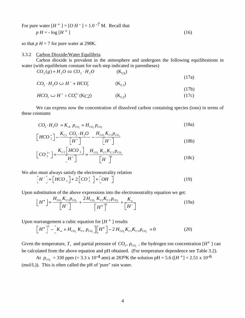
3.3.2 Carbon Dioxide/Water Equilibria

Carbon dioxide is prevalent in the atmosphere and undergoes the following equilibrations in

water (with equilibrium constant for each step indicated in parentheses)

OHCOOHgCO 2222 )( (KCh)

(17a)

322 HCOHOHCO (KC1)

(17b) 2

33 COHHCO (KC2) (KC2) (17c)

We can express now the concentration of dissolved carbon containing species (ions) in terms of

these constants

2 2 2

2 2

2 2

2 2

11 2 2

3

2 3 1 22

3 2

ch CO CO CO

CO C COC

C CO C C CO

CO H O K p H p

H K pK CO H OHCO

H H

K HCO H K K pCO

H H

(18a)

(18b)

(18c)

We also must always satisfy the electroneutrality relation

2

3 32H HCO CO OH (19)

Upon substitution of the above expressions into the electroneutrality equation we get:

2 2 2 21 1 2

2

2CO C CO CO C C CO wH K p H K K p K

HH HH

(19a)

Upon rearrangement a cubic equation for [H + ] results

2 2 2 2

3

1 1 22 0w CO C CO CO C C COH K H K p H H K K p (20)

Given the temperature, T, and partial pressure of 22 , COCO p , the hydrogen ion concentration [H+ ] can

be calculated from the above equation and pH obtained. (For temperature dependence see Table 3.2).

At 2COp = 330 ppm (= 3.3 x 10-4 atm) at 283oK the solution pH = 5.6 ([H +] = 2.51 x 10-6

(mol/L)). This is often called the pH of 'pure" rain water.

5

TABLE 3.2: Thermodynamic data for calculating temperature dependence of aqueous

equilibrium constants

3.3.3 Sulfur Dioxide/Water Equilibrium

The scenario is similar as in the case of CO2 absorption

22 2 2 2

2 2 3 1

2

3 3 2

SO

S

S

SO g H O SO H O H

SO H O H HSO K

HSO H SO K

(21a)

(21b)

(21c)

The concentrations of dissolved species are

2 2

2 2

2 2

2 2

1

3

1 22

3 2

SO SO

SO s SO

SO S S SO

SO H O H p

H K pHSO

H

H K K pSO

H

(22a)

(22b)

(22c)

Satisfying the electroneutrality relation requires

2 2 2 2

3

1 1 22 0w SO S SO SO S S SOH K H K p H H K K p (23)

The total dissolved sulfur in oxidation state + 4 is S(IV) and its concentration is given by

2 2 2

*1 1 2( )2

1 S S SSO SO S IV SO

K K KS IV H p H p

H H (24)

where *

( )S IVH is the modified Henry's constant which we can express as

2

* 2

( ) 1 1 21 10 10pH pH

S IV SO S S SH H K K K (25)

6

Clearly the modified constant H * is dependent on pH. The larger the pH, i.e the more alkaline the

solution, the larger the equilibrium content of S (IV ). This is illustrated in Figure 3.2 for

2SOp =0.2 ppb and 200 ppb.

FIGURE 3.2: Equilibrium dissolved S(IV) as a function of pH, gas-phase partial pressure

of SO2 and temperature

Let us express now mole fractions of various dissolved sulfur species as function of pH (really

these are mole ratios, i.e moles of a particular sulfur species dividied by total moles of S (IV ) or mole

fractions on water free basis since water is the dominant component.

2 2

1

3

1

23

12 2 2

0 1 1 2

3 1

1 1 2

2

13 1 2

3 2 1 2

1 10 10

1 10 10

1 10 10

pH pH

SO H O S S S

pH pH

S SHSO

pH pH

S S SSO

SO H OX K K K

S IV

HSOX K K

S IV

SOX K K K

S IV

(26a)

(26b)

(26c)

Common notation for these are 0 1 2, , in aquatic chemistry.

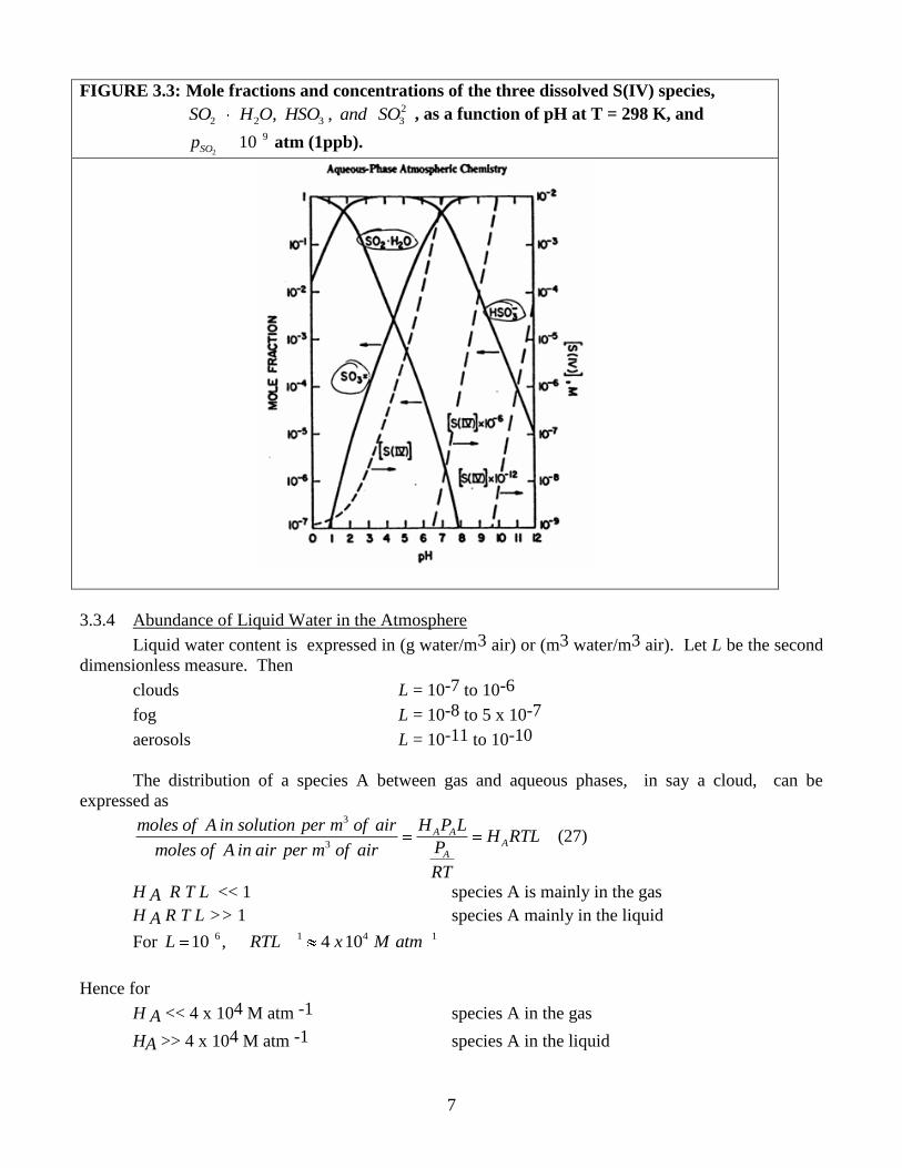
Figure 3.3 illustrates the above three mole fractions for 2

910SOp atm (1 ppb). Since these

species have different reactivities pH will affect reaction rates. At low pH 2 2SO H O dominates, at high

pH all S (IV) is in the form of 2

3SO . Intermediate pH contains mainly 3HSO .

7

FIGURE 3.3: Mole fractions and concentrations of the three dissolved S(IV) species, 2

2 2 3 3, ,SO H O HSO and SO , as a function of pH at T = 298 K, and

2

910SOp atm (1ppb).

3.3.4 Abundance of Liquid Water in the Atmosphere

Liquid water content is expressed in (g water/m3 air) or (m3 water/m3 air). Let L be the second

dimensionless measure. Then

clouds L = 10-7 to 10-6

fog L = 10-8 to 5 x 10-7

aerosols L = 10-11 to 10-10

The distribution of a species A between gas and aqueous phases, in say a cloud, can be

expressed as

3

3

A AA

A

moles of A in solution per m of air H P LH RTL

Pmoles of A in air per m of air

RT

(27)

H A R T L << 1 species A is mainly in the gas

H A R T L >> 1 species A mainly in the liquid

For 6 1 4 110 , 4 10L RTL x M atm

Hence for

H A << 4 x 104 M atm -1 species A in the gas

HA >> 4 x 104 M atm -1 species A in the liquid

8

Table 3.1 indicates that, with exception of 2 2 3, and especially and HC HCHO H O HNO , other

species will remain mainly confined to the gas phase.

For SO2 at pH = 4, * 2

( ) 10S IVH and at L = 10-6 * 1

( )S IVH RTL and most of (almost all of)

the S (IV) is in the gas phase. In contrast for H N O 3 the modified Henry's constant is

H * = 1010 and all of nitric acid is in solution.

Maximum Solubility

For example, the equilibrium dissolved concentration of A is given by e A AA H P but the total

amount of species present in a closed system (i.e. system with fixed boundaries over which no exchange

of matter occurs with the surroundings) is:

A g L

g L L

tot A g A L

L Ag A A g A

g

N C V C V

V PV C C V C L

V RT

(28)

Dividing by air volume, gV , we get:

goA

g Lo

Atot AA A

g

PN PC C L

V RT RT (29)

Since the following relationship holds

LA A AC H P (30)

Substituting eq(30) into eq(29) yields

1

1go

A AA A A

P PP H L H RTL

RT RT RT (31)

Solving for the partial pressure of A gives:

1

oA

A

A

PP

H RT L (32)

Using eq (30) we get the concentration of dissolved A in water:

1

o

L

A A

A

A

H PC

H RT L

Then, when gas solubility is very high so that 1AH RT L

the maximum concentration of dissolved A is:

max

o

L

A

A

PC

RT LmaxA (33)

Thus, essentially all of the soluble gas is in the liquid phase!

9

Clearly, then, in a closed system for a very highly soluble gas we must take precautions in calculating

the equilibrium composition not to violate the mass balance, (i.e "not to dissolve more gas than there is

available") as the concentration of eq (33) cannot be exceeded. Say PA = 10-9 atm (1 ppb) and L = 10-

6, [A]max = 4 x 10-5 M. Regardless of the value of H , say H = 1010 and [A] eq = 10 M , clearly

[A]max cannot be exceeded. [A]max can only be exceeded if the water droplets are brought into contact

with much larger volume of air not just the volume containing L amount of water.

3.4 Liquid-Liquid Systems

For immiscible liquid-liquid systems, the K-factors are known more commonly as the

distribution coefficients.

)2(

)1(

,

i

ilD

x

xK (34)

where (1) and (2) refer to liquid phases 1 and 2 with xi as the mole fraction of species i in the

corresponding phase. For gas-solid or liquid-solid systems the equilibrium is described by adsorption

equilibrium constants which will be addressed in a subsequent chapter.

Liquid-liquid equilibria can also be expressed in terms of a ratio of concentrations wo CCK

where oC is the concentration in the organic phase and

wC is the concentration in the water phase.

One important parameter widely used is environmental engineering is the octanol-water partition

coefficient usually denoted owK . This is defined as the ratio of concentration of the solute in n-octanol

to that in water. The essential idea behind the use of this parameter is that n-octanol can be viewed as

representative to the lipid phase in tissues and, hence, this quantity is a measure of how the solute gets

incorporated into the tissues. Hence accurate estimates or experimental values of this parameter is of

importance in estimating the bio-toxicity of a compound. A related parameter is the bio-concentration

factor BCF which is defined as follows:

40.0log79.0log owKBCF (35)

Thus, BCF is proportional to owK . If BCF is greater than 1000 then the compound is considered

to have a high potential for bioaccumulation. If BCF is less than 250 then the compound is assumed to

have low potential to accumulate in aquatic species.

Predictive methods based on group contributions are available for owK and these are useful as a

first estimate for a new compound in the absence of measured values.

Example: Phenol has a owKlog value of 1.46 . What is its bio-concentration potential?

Answer: Using the equation above we find log (BCF) = 0.7771

BCF = 7771.010 which is less than 250.

Hence phenol has low bio-accumulation potential.

3.5 Multiphase Distribution

Situations where multiphase equilibria, when more than two phases co-exists, need to be

assessed are optly illustrated by Figure 3.5 taken from Seader and Henley (1998) where 7 phases are

reported.

10

Air

n-hexane-rich liquid

Aniline-rich liquid

Water-rich liquid

Phosphorous liquid

Gallium liquid

Mercury liquid

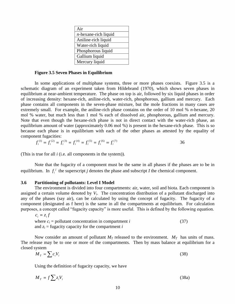
Figure 3.5 Seven Phases in Equilibrium

In some applications of multiphase systems, three or more phases coexists. Figure 3.5 is a

schematic diagram of an experiment taken from Hildebrand (1970), which shows seven phases in

equilibrium at near-ambient temperature. The phase on top is air, followed by six liquid phases in order

of increasing density: hexane-rich, aniline-rich, water-rich, phosphorous, gallium and mercury. Each

phase contains all components in the seven-phase mixture, but the mole fractions in many cases are

extremely small. For example, the aniline-rich phase contains on the order of 10 mol % n-hexane, 20

mol % water, but much less than 1 mol % each of dissolved air, phosphorous, gallium and mercury.

Note that even though the hexane-rich phase is not in direct contact with the water-rich phase, an

equilibrium amount of water (approximately 0.06 mol %) is present in the hexane-rich phase. This is so

because each phase is in equilibrium with each of the other phases as attested by the equality of

component fugacities: )7()6()5()4()3()2()1(

iiiiiii fffffff 36

(This is true for all i (i.e. all components in the system)).

Note that the fugacity of a component must be the same in all phases if the phases are to be in

equilibrium. In j

if the superscript j denotes the phase and subscript I the chemical component.

3.6 Partitioning of pollutants: Level I Model

The environment is divided into four compartments: air, water, soil and biota. Each component is

assigned a certain volume denoted by Vi. The concentration distribution of a pollutant discharged into

any of the phases (say air), can be calculated by using the concept of fugacity. The fugacity of a

component (designated as f here) is the same in all the compartments at equilibrium. For calculation

purposes, a concept called “fugacity capacity” is more useful. This is defined by the following equation.

fzc ii

where ci = pollutant concentration in compartment i (37)

and zi = fugacity capacity for the compartment i

Now consider an amount of pollutant MT released to the environment. MT has units of mass.

The release may be to one or more of the compartments. Then by mass balance at equilibrium for a

closed system

iiT VcM (38)

Using the definition of fugacity capacity, we have

iiT VzfM (38a)

11

Hence ii

T

Vz

Mf (39)

Pollutant concentration in compartment i at equilibrium is equal to

ii

iTi

Vz

zMc (40)

Pollutant total mass in any compartment i iii VcM is

ii

iiTi

Vz

VzMM (41)

Percentage distribution to compartment i is then directly calculated as

100/100 iiii

T

i VzVzM

M (42)

Note that the fugacity need not be explicitly calculated when using this approach. One needs the

information only on the fugacity capacity. We now show how these can be obtained from basic

thermodynamic properties. Also note that the above procedure can be repeated for a number of

pollutants.

3.6.1 Fugacity capacity in air phase

Fugacity of a component at ideal state in the air phase is equal to its partial pressure p, and the

concentration is equal to p/RT. Hence, using the definition of fugacity capacity

RTzair

1 (43)

which has a value of 4.04 x 10–4

mol / m3.Pa at 25ºC. The fugacity capacity in air is independent

of the chemical species and has a constant value at a fixed temperature.

3.6.2 Water phase

In aqueous systems, the fugacity of a chemical is vapPxf (44)

where x is the mole fraction and is the activity coefficient. If the solute is in equilibrium with

the gas then pf . By Henry’s law pi Hc .

Hence, we have

Hzwater (45)

where H is the Henry’s law constant in pammol 3 .

3.6.3. Soil phase

Chemicals in soil are almost always adsorbed into the natural organic matter and are in

equilibrium with the water phase concentration. Concentration in soil is related to concentration in

water by the adsorption equilibrium constant.

12

watersoilsoil cKc (46)

A measure of soilK is

ocK , the organic carbon based distribution coefficient. ocK represents the

concentration per unit mass of organic carbon in soil. If soil

represents the mass fraction of carbon in

the soil, then a measure of soilK is the product

ococK where oc

is the mass fraction of carbon.

Hence the fugacity capacity of soil is

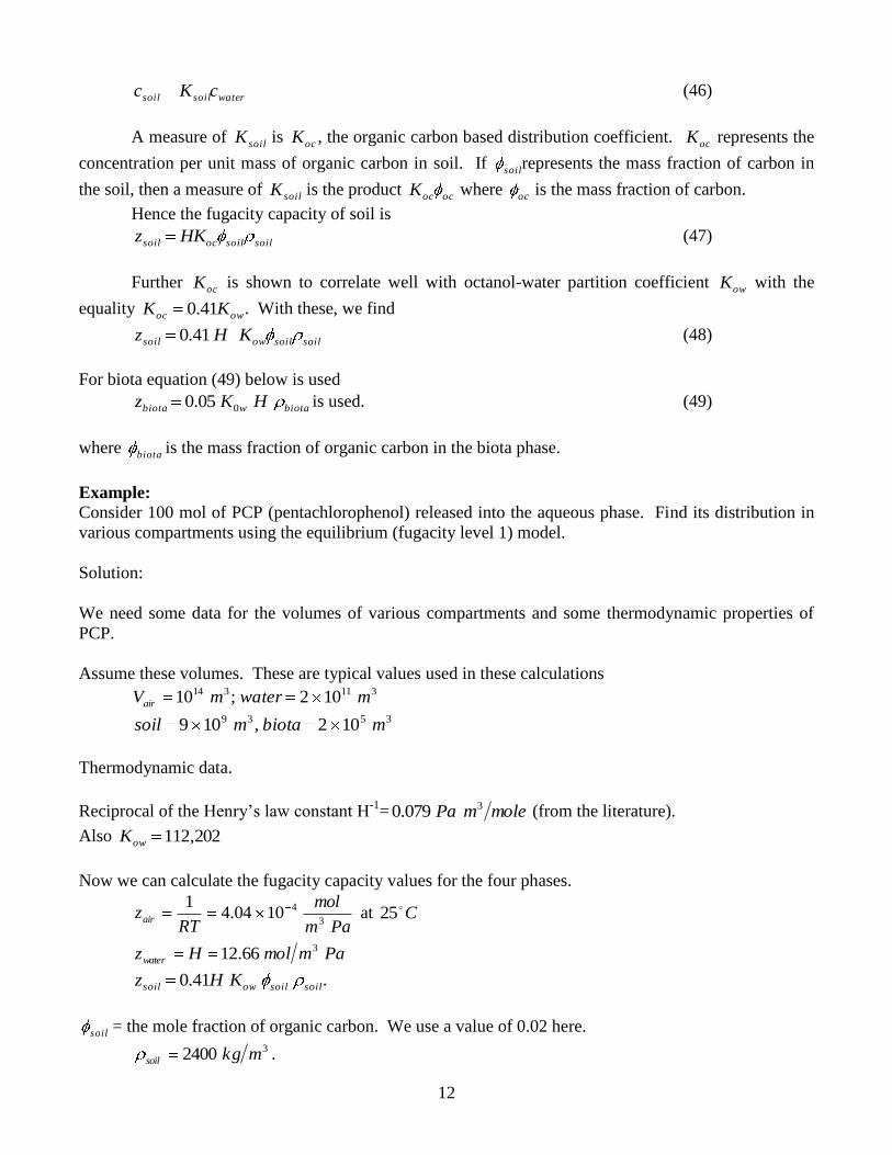
soilsoilocsoil HKz (47)

Further ocK is shown to correlate well with octanol-water partition coefficient

owK with the

equality owoc KK 41.0 . With these, we find

soilsoilowsoil KHz 41.0 (48)

For biota equation (49) below is used

biotawbiota HKz 005.0 is used. (49)

where biota

is the mass fraction of organic carbon in the biota phase.

Example:

Consider 100 mol of PCP (pentachlorophenol) released into the aqueous phase. Find its distribution in

various compartments using the equilibrium (fugacity level 1) model.

Solution:

We need some data for the volumes of various compartments and some thermodynamic properties of

PCP.

Assume these volumes. These are typical values used in these calculations 311314 102;10 mwatermVair

3539 102,109 mbiotamsoil

Thermodynamic data.

Reciprocal of the Henry’s law constant H-1

= molemPa 3079.0 (from the literature).

Also 202,112owK

Now we can calculate the fugacity capacity values for the four phases.

Pam

mol

RTzair 3

41004.41

at C25

PammolHzwater

366.12

soilsoilowsoil KHz 41.0 .

soil = the mole fraction of organic carbon. We use a value of 0.02 here. 32400 mkgsoil .

13

Using these values

Pammolzsoil

34108.2 .

Similarly we use 31000 mkgbiota and find

Pammolzbiota

34101.7 .

With all this information we can find the equilibrium of the pollutant distribution. The calculations can

be done conveniently in an excel spreadsheet or using the matlab program shown here. 341055.2 mmolvz ii

Percentage partition is then calculated as iiii vzvz and the results are

%1058.5%4.99%995.0%1059.1 32 biotaFishsoilwaterair .

PCP tends to accumulate in soil.

References:

Hilderbrand, J.H. *Principles of Chemistry, ed. MacMillian, New York, 1970.

J.D. Seader, Henley, G.J., Separation Process Principles, John Wiley & Sons, Inc., 1998.