CHAPTER 3 NUMERICAL MODELING AND MATERIAL PROPERTIES …besterfi/bascule/word_pdf/theoretical.pdf · determine the time of contact between parts of the assembly during the process

14

CHAPTER 3

NUMERICAL MODELING AND MATERIAL PROPERTIES 3.1 Introduction

An understanding of the modeling approach is necessary to appreciate the validity of the results, inherent assumptions, and consequential limitations of the parametric model. Some problems associated with the Finite Element Modeling (FEM) of thermo-structural analysis and their resolution using some non-conventional approaches are described.

Assumptions made in the model are justified based on the physics of the problem, computational time versus accuracy trade-off, limitations of finite element method, and need for simplicity. Nonlinear material properties for steel, air, and liquid nitrogen are plotted at the end of this chapter.

3.2 Coupled field analysis

Coupled field analysis involves an interaction of two or more types of phenomena. This study involves the coupling of the thermal and structural fields. ANSYS features two types of coupled field analysis: direct and indirect.

3.2.1 Direct coupled field analysis In direct coupled field analysis, degrees of freedom of multiple fields are calculated simultaneously. This method is used when the responses of the two phenomena are dependent upon each other, and is computationally more intensive. 3.2.2 Indirect coupled field (sequential coupled field analysis)

In this method, the results of one analysis are used as the loads of the following analysis. This method is used where there is one-way interaction between the two fields.

3.3 Design of the model

The sequential coupled field method described above is chosen as the approach best suited to our requirements. The underlying assumption is that the structural results are dependent upon the thermal results, but not vice-versa. This assumption is valid for the requirements of our study. Typically, this involves performing the entire thermal analysis, and subsequently transferring the thermal nodal temperatures to the structural analysis. However, our problem requires some modifications to the pure form of this approach as interaction between the two fields (thermal and structural) is required to determine the time of contact between parts of the assembly during the process of shrink-fitting. This is achieved using a non-conventional approach.

First, the thermal analysis of the cooling down of part(s) to steady state is performed. Subsequently, the structural analysis is performed to determine the time when the interference between the two parts of the assembly is breached. These parameters are used in the complete thermal analysis to switch thermal and structural contact ‘on’ and ‘off’. That is, to determine whether conductance is taking place between the parts of the assembly. The minimum temperature in the assembly during cooling down and the maximum temperature during warming up process are monitored and the

15

program exits the process in question once it nears steady state. The modeling procedure is described in the Figure 3.1.

Figure 3.1 Modeling approach.

16

In this model, we perform multiple thermal and structural analysis to determine time parameters at which certain thermal and structural criteria are met. The thermal results obtained are transferred as nodal temperatures to the structural analysis.

These parameters are used to perform the complete thermal and structural analysis along with the ancillary cooling analyses. Segments of the flowchart shown in Figure 3.1 are explained next. The section headings explain the namesake process boxes in the flowchart.

3.3.1 Cooling process 1

The phenomena modeled are: AP1 - Cooling down of the trunnion and AP2 - Cooling down of the hub

3.3.1.1 Process box-thermal analysis 1

The cooling process is performed till the user defined exit criterion for the cooling process (see Appendix B.3.5.2) is met.

Parameters output for AP1 tcoot1 - time at which the user defined exit criterion (see Appendix B.3.5.2) is

met during the cooling down of the trunnion. Parameters output for AP2

hcoot2 - time at which the user defined exit criterion (see Appendix B.3.5.2) is met during the cooling down of the hub.

3.3.1.2 Process box-structural analysis 1 The nodal temperatures from ‘thermal analysis 1’ are transferred to this analysis. The structural analysis is performed to determine the time at which the interference between the male and the female parts of the assembly is breached.

Parameters output for AP1 thct1 - time at which the interference between the trunnion and hub is

breached during the cooling down of the trunnion. Parameters output for AP2

hgct2 - time at which the interference between the hub and the girder is breached during the cooling down of the hub.

Note that thct2 and hgct2 determine the time at which the conduction between the two parts (trunnion-hub or hub-girder) of the assembly should be switched ‘on’ (see element COMBIN37 in Table 3.1). 3.3.2 Cooling process 2 The cooling down of the trunnion-hub in the case of AP1 and the cooling down of the trunnion in the case of AP2 is performed. 3.3.2.1 Process box-thermal analysis 2 The cooling process is performed till the user defined exit criterion is met. (see Appendix B.3.5.2).

17

Parameters input for AP1 thct1 - time at which the conduction between the trunnion and the hub is to

switched ‘on’. (see element COMBIN37 in Table 3.1). This parameter is obtained from ‘structural analysis 1’.

Parameters input for AP2 hgct2 - determines the time at which the conduction between the hub and the

girder is to switched ‘on’ (see element COMBIN37 in Table 3.1). This parameter is obtained from ‘structural analysis 1’.

These parameters are used to perform the thermal analysis of the second cooling process until the user defined exit criterion is met (see Appendix B.3.5.2).

Parameters output for AP1 thcoot1 - time at which the trunnion-hub assembly meets the user defined exit

criterion (see Appendix B.3.5.2) during the cooling process. twarm1 - time at which the trunnion-hub assembly meets the user defined exit

criterion (see Appendix B.3.5.2) during the warming up of the trunnion.

Parameters output for AP2 tcoot2 - the time at which the user defined exit criterion (see Appendix B.3.5.2)

during the cooling down of the trunnion is met. hwarm2 - the time at which the user defined exit criterion (see Appendix B.3.5.2)

during the warming up of the hub is met.

3.3.2.2 Process box-structural analysis 2 The nodal temperatures from ‘thermal analysis 2’ are transferred to this analysis. The structural analysis is performed to determine the time at which the interference between the two parts of the assembly is breached.

Parameters output for AP1 hgct1 - time at which the interference between the trunnion-hub and the girder

is breached. Parameters output for AP2

thct2 - time at which the interference between the trunnion and the hub-girder assembly is breached.

3.3.3 Complete analysis

Parameters obtained from previous thermal and structural analysis are used to perform the complete thermal and structural analysis.

3.3.3.1 Process box-full thermal analysis

Parameters input for AP1 thct1 - see previous sections hgct1 - see previous sections twarm1 - see previous sections

Parameters input for AP2 hgct2 - see previous sections thct2 - see previous sections hwarm2 - see previous sections

18

Parameters output for AP1 thwarm1 - the time at which the THG assembly meets the user defined exit

criterion when the trunnion-hub assembly is fitted into the girder (see Appendix B.3.5.2).

Parameters output for AP2 twarm2 - the time at which the THG assembly meets the user defined exit

criterion when the trunnion is fitted into the hub-girder assembly (see Appendix B.3.5.2).

3.3.3.2 Process box-full structural analysis The nodal temperatures from ‘full thermal analysis’ are transferred to this analysis. The complete structural analysis is performed for both the assembly procedures. 3.3.4 Ancillary analysis The stand alone cooling down processes are performed. 3.3.4.1 Ancillary cooling 1 The following cooling process in performed: for AP1 - cooling down of the trunnion, and for AP2 - cooling down of the hub. 3.3.4.2 Ancillary cooling 2 The following cooling process is performed: for AP1 - cooling down of the trunnion-hub, and for AP2 - cooling down of the trunnion

Parameters input for AP1 thct1 - time of contact between the trunnion and the hub (see Appendix

B.3.5.2). This parameter is obtained from ‘structural analysis 1’. twarm1 - time at which the trunnion-hub assembly fulfills user defined exit

criterion (see Appendix B.3.5.2) during the insertion of the trunnion into the hub.

Parameters input for AP2 hgct2 - time of contact between the hub and the girder. This parameter is

obtained from ‘structural analysis 1’. hwarm2 - time at which the hub-girder assembly fulfills user defined exit

criterion during the insertion of the hub into the girder.

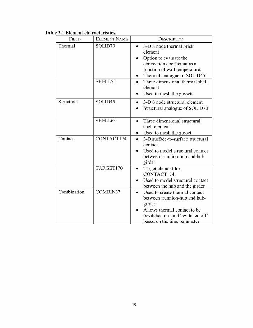
3.4 The finite element model Table 3.1 describes the types of element used in the model with a brief description

of each. The structural and thermal element meshes for the THG assembly are shown in Figure 3.2a (brick elements) and Figure 3.2b (shell elements). Note that the sequential coupled field analysis requires separate elements to be defined for both the thermal and structural analysis. Hence, Figure3.2a and Figure 3.2b plot both the thermal and the structural elements at the same time. The shell elements used to plot the gussets are shown in Figure 3.2b. Figure 3.2c plots the contact and target elements and Figure 3.2d plots the combination elements.

19

Table 3.1 Element characteristics. FIELD ELEMENT NAME DESCRIPTION

SOLID70 • 3-D 8 node thermal brick element

• Option to evaluate the convection coefficient as a function of wall temperature.

• Thermal analogue of SOLID45

Thermal

SHELL57 • Three dimensional thermal shell element

• Used to mesh the gussets SOLID45 • 3-D 8 node structural element

• Structural analogue of SOLID70 Structural

SHELL63 • Three dimensional structural shell element

• Used to mesh the gusset Contact CONTACT174 • 3-D surface-to-surface structural

contact. • Used to model structural contact

between trunnion-hub and hub girder

TARGET170 • Target element for CONTACT174.

• Used to model structural contact between the hub and the girder

Combination COMBIN37 • Used to create thermal contact between trunnion-hub and hub-girder

• Allows thermal contact to be ‘switched on’ and ‘switched off’ based on the time parameter

20

Figure 3.2a Thermal element SOLID70 and structural element SOLID45.

Figure 3.2b Thermal element SHELL57 and structural element SHELL63.

21

Figure 3.2c Contact elements CONTACT174 and TARGET170.

Figure 3.2d COMBIN37 elements.

22

3.5 Assumptions 3.5.1 Sequential coupled field approach

The assumption in this approach is that the structural results are dependent upon the thermal results but not vice-versa. This is a fair assumption as the effect of strains on the thermal analysis is negligible.

3.5.2 Convection coefficient

The assumptions in the calculation of the convective heat transfer coefficient for air are:

1. The geometry of the assemblies is assumed to cylindrical. To obtain the convective heat transfer coefficient, the Grashoff’s number (Gr ), Prandtl number ( Pr ), and the Nusselt number ( Nu ) are required. The equations to obtain these quantities are discussed next. Grashoff’s number is defined by Ozisik (1977) as

3

3)(ν

β DTTgGr w ∞−= (3.1a)

where g = acceleration due to gravity, β = volume coefficient of thermal expansion, wT = wall temperature, ∞T = ambient temperature, D = diameter of cylinder, and ν = kinematic viscosity. The Prandtl number, Pr is defined by Ozisik (1977) as

k

c p µ=Pr (3.1b)

where cp = specific heat, µ = absolute viscosity, and k = coefficient of thermal conductivity. The Nusselt’s number, Nu is defined by the following equation (Ozisik, 1977). 3/1Pr)(53.0 GrNu = . (3.1c) The convective heat transfer coefficient, hm is also obtained from Ozisik (1977) as

D

kNuhm = . (3.1d)

2. The value for the hydraulic diameter, D, for the trunnion is the outer diameter of the trunnion; for the hub, it is the hub outer diameter; and for the girder, it is the length of the girder.

3. Turbulent flow is assumed. 4. The convection coefficient is assumed to be dependent on the wall,

temperature and the bulk or ambient temperature.

23

The convection coefficient for air is plotted later in this chapter. Note that the value for the convective heat transfer coefficient is not a function of the hydraulic diameter. Hence, the convective coefficient is independent of the bridge geometry. 3.5.3 Time increments and contact point The minimum time increment in this model is one minute. Hence, the degree of accuracy of our time of contact between parts of the assembly is less than one minute. 3.5.4 Finite element method assumptions The standard inaccuracies associated with any finite element model due to mesh density, time increments, number of substeps, etc. are present in this model (Logan, 1996). 3.5.5 Material properties The material properties of the THG assembly, the air, and the cooling medium are temperature dependent and are evaluated at specified temperature increments. The properties in between or outside the extremes of these values are interpolated and extrapolated, respectively. 3.6 Nonlinear material properties of metal

The nonlinear material properties for a typical steel - Fe - 2.25 Ni (ASTM A203-A) are plotted in the next several pages. Though nonlinear material properties in general are explored, particular emphasis is given to properties at low temperatures.

3.6.1 Young’s modulus

The elastic modulus of all metals increases monotonically with increase in temperature. The elastic modulus TE can be fitted into a semi-empirical relationship:

]1)/[exp( −−=

TTSEE

eoT (3.2)

where 0E = elastic constant at absolute zero, S = constant, and eT = Einstein characteristic temperature.

The Young’s modulus remains stable with change in temperature (see Figure 3.3) and hence is assumed to remain constant throughout this analysis.

24

0

5

10

15

20

25

30

35

-400 -300 -200 -100 0 100Temperature (oF)

Youn

g's

Mod

ulus

(Mps

i)

Figure 3.3 Young’s modulus of steel as a function of temperature. 3.6.2 Coefficient of thermal expansion

The coefficient of thermal expansion at different temperatures is determined principally by thermodynamic relationships with refinements accounting for lattice vibration and electronic factors. The electronic component of coefficient of thermal expansion becomes significant at low temperatures in cubic transition metals like iron (Reed, 1983). The coefficient of thermal expansion increases with increase in temperature by a factor of three from –3210F to 800F as shown in the Figure 3.4.

0

1

2

3

4

5

6

7

-400 -300 -200 -100 0 100Temperature (oF)

Coe

ffici

ent o

f The

rmal

Exp

ansi

on(1

0-6 in

/in/o F)

Figure 3.4 Coefficient of thermal expansion of steel as a function of temperature.

25

3.6.3 Thermal conductivity The coefficient of thermal conductivity (see Figure 3.5) increases with an increase

in temperature by a factor of two from –3210F to 800F. Thermal conduction takes place via electrons, which is limited by lattice imperfections and phonons. In alloys, the defect scattering effect ( )T∝ is more significant than the phonon scattering effect ( )2−∝ T (Reed, 1983).

0.0

0.4

0.8

1.2

1.6

2.0

-400 -300 -200 -100 0 100Temperature (oF)

Ther

mal

Con

duct

ivity

(BTU

/hr/i

n/o F)

Figure 3.5 Thermal conductivity of steel as a function of temperature. 3.6.4 Density

For the range of temperatures of interest to our study the density remains nearly constant, as shown in Figure 3.6.

0.00

0.05

0.10

0.15

0.20

0.25

0.30

-400 -300 -200 -100 0 100Temperature (oF)

Den

sity

(lb/in

3 )

Figure 3.6 Density of steel as a function of temperature.

26

3.6.5 Specific heat Lattice vibrations and electronic effects affect the specific heat of a material. The contribution of two effects can be shown by

TTC γβ += 3 (3.3) where, 3Tβ = lattice contribution, β = volume coefficient of thermal expansion, Tγ = electronic contribution, and γ = normal electronic specific heat. Note that specific heat decreases by a factor of five over the temperature range in question, as shown in Figure 3.7.

0.00

0.02

0.04

0.06

0.08

0.10

0.12

-400 -300 -200 -100 0 100

Temperature (oF)

Spec

ific

Hea

t(B

TU/lb

/o F)

Figure 3.7 Specific heat of steel as a function of temperature. 3.7 Nonlinear material properties of air and liquid nitrogen The temperature dependent convective heat transfer coefficients for air and liquid nitrogen are plotted next. 3.7.1 Convection to air at 800F

The convective heat transfer coefficient is a function of the volume coefficient of thermal expansion ( β ), the thermal conductivity ( k ), absolute viscosity ( µ ), kinematic viscosity (ν ), specific heat ( pc ) and mass density ( ρ ) all of which are temperature dependent. The Grashof number, the Nusselt number and the Prandtl number and ultimately the convective heat transfer coefficient can be calculated from these quantities from Equations (3.1a) through (3.1d). The variation of each with temperature is plotted in Figure 3.8a through Figure 3.8f.

27

0.0000

0.0005

0.0010

0.0015

0.0020

0.0025

0.0030

-400 -300 -200 -100 0 100Temperature (oF)

Volu

me

Ther

mal

Exp

ansi

on(1

0-6 m

3 /m3 /o F)

Figure 3.8a Volume coefficient of thermal expansion of air as a function of

temperature.

0.0000

0.0002

0.0004

0.0006

0.0008

0.0010

0.0012

0.0014

-400 -300 -200 -100 0 100Temperature (oF)

Ther

mal

Con

duct

ivity

(BTU

/hr/i

n/o F)

Figure 3.8b Thermal conductivity of air as a function of temperature.

28

0

20

40

60

80

100

-400 -300 -200 -100 0 100

Temperature (oF)

Kine

mat

ic V

isco

sity

(in2 -h

r)

Figure 3.8c Kinematic viscosity of air as a function of temperature.

0.000

0.050

0.100

0.150

0.200

0.250

-400 -300 -200 -100 0 100

Temperature (oF)

Spec

ific

Hea

t(B

TU/lb

/o F)

Figure 3.8d Specific heat of air as a function of temperature.

29

0.0000

0.0005

0.0010

0.0015

0.0020

0.0025

0.0030

0.0035

0.0040

-400 -300 -200 -100 0 100

Temperature(oF)

Abso

lute

Vis

cosi

ty(lb

/in/h

r)

Figure 3.8e Absolute viscosity of air as a function of temperature.

0.00000

0.00002

0.00004

0.00006

0.00008

0.00010

0.00012

0.00014

0.00016

0.00018

-400 -300 -200 -100 0 100

Temperature (oF)

Mas

s D

ensi

ty(lb

/in3 )

Figure 3.8f Mass density of air as a function of temperature. The convective heat transfer coefficient for air, based upon the previous five graphs (see Figures 3.8b through 3.8f) and Equations (3.1), is shown in Figure 3.8g. Note that the convective heat transfer coefficient for convection to air is evaluated at the film temperature (that is, the average of the bulk and the wall temperatures).

30

0.000

0.002

0.004

0.006

0.008

0.010

0.012

0.014

-400 -300 -200 -100 0 100

Film Temperature (oF)

Con

vect

ive

Hea

t Tra

nsfe

r Coe

ffici

ent

(BTU

/hr/o F/

in2 )

Figure 3.8g Convective heat transfer coefficient of air as a function of temperature. 3.7.2 Convection to liquid nitrogen at –3210F

The phenomenon of convection to liquid nitrogen is quite complex and involves multi-phase heat transfer. Whenever an object at ambient temperature (that is, 800F) comes into contact with liquid nitrogen “film boiling” occurs until the temperature of the object reaches approximately –2600F. This phenomenon of film boiling occurs when there is a large temperature difference between the cooling surface and the boiling fliud. At the point when film boiling stops, the minimum heat flux occurs and the phenomenon of “transition boiling” occurs until the temperature of the object reaches –2900F. At the point when transition boiling stops, the maximum heat flux occurs and the phenomenon of “nucleate boiling” occurs until the temperature of the object reaches the temperature of liquid nitrogen. Nucleate boiling occurs when small bubbles are formed at various nucleation sites on the cooling surface. When nucleate boiling starts the object cools very rapidly.

The convective heat transfer coefficient for convection to liquid nitrogen is dependent on many factors, such as, surface finish, size of the object and shape of the object, to name a few. Based on the previous discussion, the convective heat transfer coefficient for convection to liquid nitrogen is shown in Figure 3.9 (Brentari and Smith 1964). This data was chosen because it very closely matches the surface finish, and object sizes and shapes used for trunnions and hubs. Note that the convective heat transfer coefficient for convection to liquid nitrogen is evaluated at the wall temperature.

31

0.48

0.50

0.52

0.54

0.56

0.58

0.60

-400 -300 -200 -100 0 100

Wall Temperature (oF)

Con

vect

ive

Hea

t Tra

nsfe

r Coe

ffici

ent

(BTU

/hr/o F/

in2 )

Figure 3.9 Convective heat transfer coefficient of liquid nitrogen as a function of

temperature.

17.37

0.069

32

CHAPTER 4

SUMMARY OF RESULTS FOR PARAMETRIC FEA (PHASE I)

4.1 Introduction The results of the study are presented in this chapter. Theories of failure based on

fracture mechanics and yield stresses present several alternative causes of failure. The relevant theory for crack formation in the Trunnion-Hub-Girder (THG) was formulated based on several observations. First, the steady state stresses after assembly were well below the yield point and could not have caused failure. Second, experimental observations indicate the presence of small cracks in the assembly. Last, cracks were formed during the immersion of the trunnion-hub assembly in liquid nitrogen. This observation is important as fracture toughness decreases with a decrease in temperature whereas yield strength increases with a decrease in temperature (see Figure 4.1b). Our hypothesis is that the small cracks present in the assembly propagate catastrophically once the size of the crack exceeds the critical crack length. This hypothesis is tested using the THGTM (Trunnion-Hub-Girder Testing Model). A brief explanation of this theory is included. Time history plots of temperatures, hoop stresses and critical crack lengths at different stages in the assembly process are presented. The plots show the interdependence of the variables and suggest possible avenues of optimizing them by changing the parameters or steps involved in the assembly process. One possible solution, using AP2, is explored and a comparison between the two assembly procedures for different bridges is presented. A phenomenon called crack arrest, that may prevent cracking in some cases despite low critical crack lengths, is described and the possibility of it occurring is explored.

The results are important from two perspectives, one of which is explicitly presented in the results and the other which is implicitly suggested. The explicit result is the comparison between the two assembly procedures. Also, implicitly presented in the results is a comparison of different bridges explaining why some THG assemblies form cracks while others do not.

4.2 Bridge geometric parameters

The geometric parameters for the three bridges, that are, Christa McAuliffe Bridge, Hillsborough Avenue Bridge and 17th Street Causeway Bridge, are presented in Table 4.1a. For a schematic and description of the parameters, refer to Figures B.13a, B.14a, and B.15a of Appendix B. Interference values for FN2 fits can be obtained from the Bascule Bridge Design Tools (Denninger, 2000). In this study, we analyze the worst case, that is, maximum interference between the trunnion and hub, and minimum interference between the hub and the girder. These values of interference will cause the largest tensile hoop stress in the hub. The interference values, based on FN2 fits, used in this analysis are presented in Table 4.1b.

33

Table 4.1a Geometric parameters. BRIDGE

GEOMETRIC PARAMETERS

CHRISTA MCAULIFFE

HILLSBOROUGH AVENUE

17TH STREET CAUSEWAY

hgf (in) 1.5 1 0.75 hgw (in) 82 90 60

l (in) 18.5 20 6 lf (in) 4.25 8.5 4.25 lg (in) 82 90 60 lh (in) 16 22 11 lt (in) 53.5 62 23

rhg (in) 16 15.39 8.88 rho (in) 27 24.5 13.1825 rti (in) 1 1.125 1.1875 rto (in) 9 8.39 6.472 tg (in) 1.5 1.5 1.25

wbr (in) 1.75 1.75 0.78125 wgf (in) 17 14 1.25 wgw (in) 1.5 1 0.75 whf (in) 1.75 1.75 1.25

Table 4.1b Interference values.

BRIDGE DIAMETRICAL INTERFERENCE

CHRISTA MCAULIFFE

HILLSBOROUGH AVENUE

17TH STREET CAUSEWAY

Trunnion-Hub (in) 0.008616 0.008572 0.007720 Hub-Girder (in) 0.005746 0.005672 0.004272

4.3 Bridge loading parameters

The material properties of an equivalent metal, that is, Fe - 2.25 Ni (ASTM A203-A), are presented in Chapter 3. Also presented are the thermal properties of air and liquid nitrogen. Bulk temperatures used for the results presented are given in Table 4.2.

Table 4.2 Bulk temperatures.

TYPE OF BULK TEMPERATURE

TEMPERATURE (0F)

Ambient air bulk temperature 85 Cooling medium bulk temperature -321

4.4 Convergence test and result verification

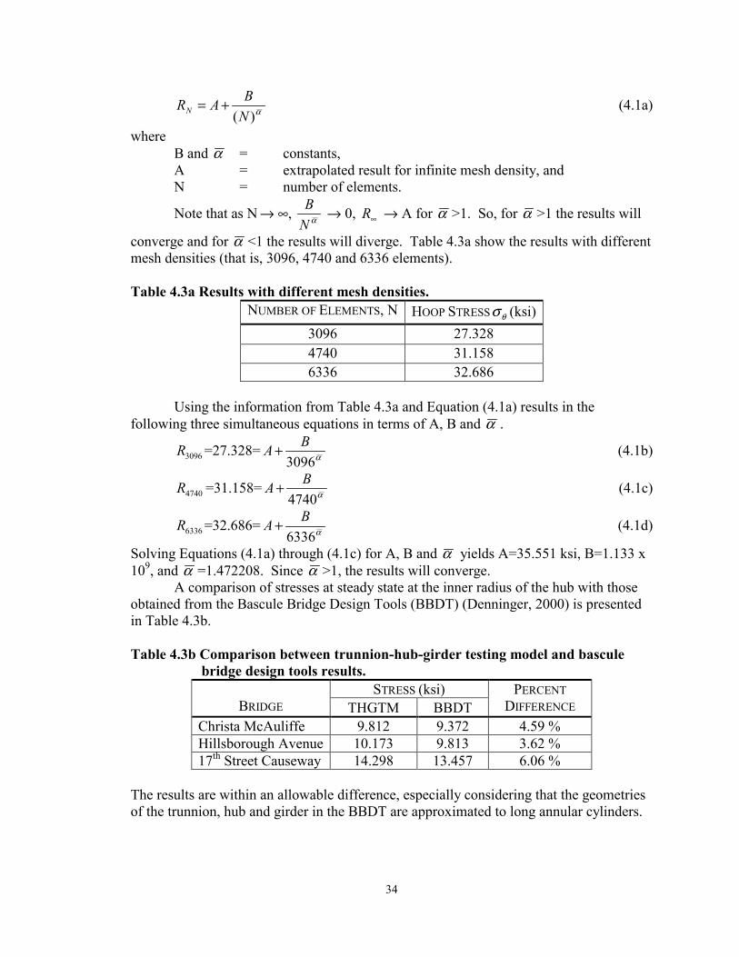
A convergence test is performed to verify the suitability of the mesh used in the analysis. The hoop stress is calculated at different levels of meshing, that is, different mesh densities. The hoop stress, NR , at a point (Logan, 1992) is given by

34

α)(NBARN += (4.1a)

where B and α = constants, A = extrapolated result for infinite mesh density, and N = number of elements.

Note that as N → ∞, αNB → 0, ∞R → A for α >1. So, for α >1 the results will

converge and for α <1 the results will diverge. Table 4.3a show the results with different mesh densities (that is, 3096, 4740 and 6336 elements). Table 4.3a Results with different mesh densities.

NUMBER OF ELEMENTS, N HOOP STRESS θσ (ksi) 3096 27.328 4740 31.158 6336 32.686

Using the information from Table 4.3a and Equation (4.1a) results in the following three simultaneous equations in terms of A, B and α .

3096R =27.328= α3096BA + (4.1b)

4740R =31.158= α4740BA + (4.1c)

6336R =32.686= α6336BA + (4.1d)

Solving Equations (4.1a) through (4.1c) for A, B and α yields A=35.551 ksi, B=1.133 x 109, and α =1.472208. Since α >1, the results will converge. A comparison of stresses at steady state at the inner radius of the hub with those obtained from the Bascule Bridge Design Tools (BBDT) (Denninger, 2000) is presented in Table 4.3b. Table 4.3b Comparison between trunnion-hub-girder testing model and bascule

bridge design tools results. STRESS (ksi)

BRIDGE THGTM BBDT PERCENT

DIFFERENCE Christa McAuliffe 9.812 9.372 4.59 % Hillsborough Avenue 10.173 9.813 3.62 % 17th Street Causeway 14.298 13.457 6.06 %

The results are within an allowable difference, especially considering that the geometries of the trunnion, hub and girder in the BBDT are approximated to long annular cylinders.

35

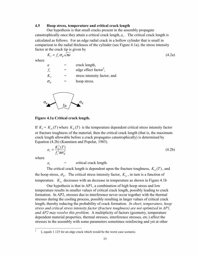
4.5 Hoop stress, temperature and critical crack length Our hypothesis is that small cracks present in the assembly propagate catastrophically once they attain a critical crack length, ca . The critical crack length is calculated as follows. For an edge radial crack in a hollow cylinder that is small in comparison to the radial thickness of the cylinder (see Figure 4.1a), the stress intensity factor at the crack tip is given by afK eI πσθ= (4.2a) where

a = crack length, ef = edge effect factor3,

IK = stress intensity factor, and

θσ = hoop stress. Figure 4.1a Critical crack length. If IK = )(TKIc where )(TKIc is the temperature dependent critical stress intensity factor or fracture toughness of the material, then the critical crack length (that is, the maximum crack length allowable before a crack propagates catastrophically) is determined by Equation (4.2b) (Kanninen and Popelar, 1985).

22

2 )(θπσe

Icc f

TKa = (4.2b)

where ca = critical crack length.

The critical crack length is dependent upon the fracture toughness, )(TKIc , and the hoop stress, θσ . The critical stress intensity factor, IcK , in turn is a function of temperature. IcK decreases with an decrease in temperature as shown in Figure 4.1b Our hypothesis is that in AP1, a combination of high hoop stress and low temperature results in smaller values of critical crack length, possibly leading to crack formation. In AP2, stresses due to interference never occur together with the thermal stresses during the cooling process, possibly resulting in larger values of critical crack length, thereby reducing the probability of crack formation. In short, temperature, hoop stress and critical stress intensity factor (fracture toughness) are not optimized in AP1, and AP2 may resolve this problem. A multiplicity of factors (geometry, temperature dependent material properties, thermal stresses, interference stresses, etc.) affect the stresses in the assembly with some parameters sometimes reinforcing and yet at other 3 fe equals 1.125 for an edge crack which would be the worst case scenario.

θσ θσa

36

times negating the effects of each other. Therefore, this intuitive analysis needs to stand the test of a numerical model before gaining engineering acceptability. The THGTM is used for this purpose.

Figure 4.1b Fracture toughness and temperature (Blair et al., 1995). The THGTM is used to plot the temperature, hoop stress and the critical crack length at possible points of failure in the assembly. The critical crack length is used as the parameter for comparison between different assembly procedures for different bridges. A further study possible with the THGTM (though not included as a part of this study) is analyzing the effect of the different loading parameters on the critical crack length. 4.6 Transient stresses and critical crack length using the trunnion-hub-girder

testing model The THGTM is used to analyze the stresses and critical crack length at possible locations of failure. We choose the point with the greatest probability of failure and plot critical crack lengths, hoop stress and temperature against time for that point.

With the aim of modeling the worst case from the perspective of failure (see Section 4.12) in our model, the male parts of the assembly are inserted into the female parts as soon as the interference between the two is breached. In practice, it is often difficult to shrink-fit an assembly without a clearance, and hence the high stresses after contact may not be observed in practice. It is important to note that in practice it is impossible to perform an insertion without a gap and hence the high stresses noticed immediately after contact may not be observed in practice. Also, the entire assembly process and the ancillary cooling processes are performed separately. Hence, the time periods for which the cooling is performed in the full assembly process (only till interference is breached) will be different from that in the ancillary cooling process (user specified cooling time).

37

The results are presented with time-history plots for all the bridges. Selected contour plots are presented only for the Christa McAuliffe Bridge. 4.7 Christa McAuliffe Bridge

Possible critical points in the hub are studied using the THGTM. The element at the inner radius of the hub on the gusset side is found to be the most critical element. Figure 4.2 shows the chosen element.

Figure 4.2 Front and side view of the chosen element in the Christa McAuliffe hub. 4.7.1 Assembly procedure 1 (AP1) 4.7.1.1 Full assembly process The stresses, temperatures and critical crack lengths during AP1 are plotted against time in Figure 4.3. The time period for which each step of the assembly process is performed is given in Table 4.4.

Element

38

Figure 4.3 Critical parameters (CCL is critical crack length in inches, TEMP is

temperature in 0F, and HOOP is hoop stress in psi) plotted against time (full assembly process during AP1 of Christa McAuliffe Bridge).

Table 4.4 Time for each step of AP1 for the Christa McAuliffe Bridge.

STEP

STARTING TIME (min)

ENDINGTIME (min)

Cooling down of the trunnion 0 3 Sliding the trunnion into the hub 4 503 Cooling down the trunnion-hub assembly 504 505 Sliding the trunnion-hub assembly into the girder 506 1705

4.7.1.2 Cooling down of the trunnion

The stresses at the hub are not affected during this step.

4.7.1.3 Sliding the trunnion into the hub The hoop stress, temperature and the critical crack length during this step are

plotted against time in Figure 4.4. Almost immediately after contact, a combination of interference and thermal stresses produces high hoop stresses at the inner radius of the hub. Due to the effects of conduction and convection, the temperatures in the trunnion-hub assembly begin to converge to around the same temperature. As a consequence, the thermal stresses play an increasingly marginal role with the passage of time.

39


temperature in 0F, and HOOP is hoop stress in psi) plotted against time (sliding the trunnion into the hub during AP1 of the Christa McAuliffe Bridge).

Though this step is not important from the perspective of failure, as the critical crack lengths are high, an interesting interplay of temperatures, hoop stresses and critical crack length can be seen. As temperature and hoop stress fall, the critical crack length initially falls before rising. (see Equation (4.2b)). 4.7.1.4 Cooling down the trunnion-hub assembly

The hoop stress, temperature and the critical crack length during this step are plotted against time in Figure 4.5a. The results from the THGTM indicate that the lowest values of critical crack length during AP1 are observed during this step. This result is supported by experimental observation of crack formation during this step (see Chapter 1). This assumes special significance as Christa McAuliffe is one of the bridges that formed cracks during this step. Furthermore, the critical crack length remains low for a considerable period of time in contrast to what is observed in AP2 during its counterpart critical step: cooling of the hub (see Appendix B.7.2.2). This behavior assumes importance in our discussion of crack arrest (see Section 4.11). Initially, thermal and interference stresses reinforce each other and high hoop stresses occur as a result. As the trunnion-hub assembly nears steady state, the stresses due to interference dominate.

40

Figure 4.5a Critical parameters (CCL is critical crack length in inches, TEMP is

temperature in 0F, and HOOP is hoop stress in psi) plotted against time (cooling down of the trunnion-hub assembly during AP1 of the Christa McAuliffe Bridge).

Contour plots of the hoop stress and the temperature in the hub when the highest

hoop stress is noticed are plotted in Figures 4.5b and 4.5c, respectively. Hoop stress and temperature plots when the lowest critical crack is observed are plotted in Figures 4.5d and 4.5e, respectively.

41

Figure 4.5b Hoop stress (psi) plot when the highest hoop stress during AP1 is

observed.

Figure 4.5c Temperature (0F) plot when the highest hoop stress during AP1 is

observed.

42

Figure 4.5d Hoop stress (psi) plot when the lowest critical crack length during AP1

is observed.

Figure 4.5e Temperature (0F) plot when the lowest critical crack length during AP1

is observed.

43

4.7.1.5 Sliding the trunnion-hub assembly into the girder The hoop stress, temperature and the critical crack length during this step are

plotted against time in Figure 4.6 for this step. During this step, hoop stresses remain fairly stable primarily due to the remoteness of the inner radius of the hub from the hub girder interface. A rise in the temperature due to conduction and convection is accompanied initially with a rise, and later a fall in the hoop stress, confirming the somewhat non-intuitive behavior of thermal stresses. High values of the critical crack length indicate the low probability of crack propagation during this step.


temperature in 0F, and HOOP is hoop stress in psi) plotted against time (sliding the trunnion–hub assembly into the girder during AP1 of Christa McAuliffe Bridge).

4.7.2 Assembly Procedure 2 (AP2) 4.7.2.1 Full assembly process The stresses, temperatures and critical crack lengths at the chosen element are plotted against time in Figure 4.7. The time period for which each step of the assembly process is performed is given in Table 4.5.

44


temperature in 0F, and HOOP is hoop stress in psi) plotted against time (full assembly process during AP2 of Christa McAuliffe Bridge).

Table 4.5 Time for each step of AP2 for the Christa McAuliffe Bridge.

STEP

STARTING TIME (min)

ENDINGTIME (min)

Cooling down of the hub 0 2 Sliding the hub into the girder 3 202 Cooling down the trunnion 203 208 Sliding the trunnion into the hub-girder assembly 209 2158

4.7.2.2 Cooling down of the hub

The stresses, temperatures and critical crack lengths during this step are plotted against time in Figure 4.8a. A sharp thermal gradient across the radius at the inner radius of the hub initially results in high values of hoop stress. Over time, as the temperature gradient becomes less steep, the hoop stresses fall. The lowest value of critical crack length in AP2 is observed during this step. Note that the critical crack length rises almost instantaneously after reaching its lowest point indicating a possibility of crack arrest (see Section 4.11)

45

Figure 4.8a Critical parameters (CCL is critical crack length in inches, TEMP is

temperature in 0F, and HOOP is hoop stress in psi) plotted against time (cooling down of the hub during AP2 of the Christa McAuliffe Bridge).

Contour plots of the hoop stress and the temperature in the hub when the highest hoop stress is noticed are plotted in Figures 4.8b and 4.8c, respectively. Hoop stress and temperature plots when the lowest critical crack is observed are plotted in Figures 4.8d and 4.8e, respectively.

46

Figure 4.8b Hoop stress (psi) plot when the highest hoop stress during AP2 is

observed.

Figure 4.8c Temperature (0F) plot when the highest hoop stress during AP2 is

observed.

47

Figure 4.8d Hoop stress (psi) plot when the lowest critical crack length during AP2

is observed.

Figure 4.8e Temperature (0F) plot when the lowest critical crack length during AP2

is observed.

48

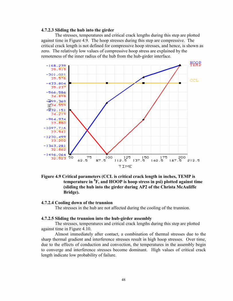
4.7.2.3 Sliding the hub into the girder The stresses, temperatures and critical crack lengths during this step are plotted

against time in Figure 4.9. The hoop stresses during this step are compressive. The critical crack length is not defined for compressive hoop stresses, and hence, is shown as zero. The relatively low values of compressive hoop stress are explained by the remoteness of the inner radius of the hub from the hub-girder interface.


temperature in 0F, and HOOP is hoop stress in psi) plotted against time (sliding the hub into the girder during AP2 of the Christa McAuliffe Bridge).


The stresses in the hub are not affected during the cooling of the trunnion. 4.7.2.5 Sliding the trunnion into the hub-girder assembly

The stresses, temperatures and critical crack lengths during this step are plotted against time in Figure 4.10.

Almost immediately after contact, a combination of thermal stresses due to the sharp thermal gradient and interference stresses result in high hoop stresses. Over time, due to the effects of conduction and convection, the temperatures in the assembly begin to converge and interference stresses become dominant. High values of critical crack length indicate low probability of failure.

49


temperature in 0F, and HOOP is hoop stress in psi) plotted against time (sliding the trunnion into the hub-girder assembly during AP2 of the Christa McAuliffe Bridge).

50

4.8 Hillsborough Avenue Bridge Possible critical points are studied in the hub using the THGTM. The element at

the inner radius of the hub on the backing ring side is found to be the most critical. Figure 4.11 shows the chosen element in the hub.

Figure 4.11 Front and side view of the chosen element in the Hillsborough Avenue

hub 4.8.1 Assembly procedure 1 (AP1) 4.8.1.1 Full assembly process The hoop stresses, temperatures and critical crack lengths at the chosen element are plotted against time in Figure 4.12. Time period for each step of the assembly process is performed is listed in Table 4.6.

Element

51


temperature in 0F, and HOOP is hoop stress in psi) plotted against time (full assembly process during AP1 of the Hillsborough Avenue Bridge).

Table 4.6 Time for each step of AP1 for the Hillsborough Avenue Bridge.

STEP

STARTING TIME (min)

ENDINGTIME (min)



The stresses in the hub are not affected during the cooling down of trunnion.

4.8.1.3 Sliding the trunnion into the hub The hoop stresses, temperatures and the critical crack lengths during this step are

plotted against time in Figure 4.13. A combination of stresses due to a sharp thermal gradient and interference

stresses result in high hoop stresses after contact. As the temperature in the assembly becomes constant due to the effects of conduction and convection, stresses due to interference dominate. High values of critical crack length indicate low probability of failure.

52


temperature in 0F, and HOOP is hoop stress in psi) plotted against time (sliding the trunnion into the hub during AP1 of the Hillsborough Avenue Bridge).

4.8.1.4 Cooling down the trunnion-hub assembly

The hoop stress, temperature and the critical crack length during this step are plotted against time in Figure 4.14. The results from the THGTM indicate that the lowest values of critical crack length during AP1 are observed during this step. Initially, thermal and structural stresses reinforce each other and high hoop stresses occur as a result. As the trunnion-hub assembly nears steady state, the stresses due to interference dominate. The trends of stresses and critical crack length are similar to what is observed in the Christa McAuliffe Bridge. The critical crack length remains low after its initial decline and shows no distinct upward trend noticed during the cooling of the hub in AP2 (see Appendix B.8.2.2). The highest value of hoop stress and lowest value of critical crack length occur almost together (though not precisely so, indicating a strong relationship between the two quantities).

53


temperature in 0F, and HOOP is hoop stress in psi) plotted against time (cooling down of the trunnion-hub during AP1 of the Hillsborough Avenue Bridge).

4.8.1.5 Sliding the trunnion-hub assembly into the girder

The hoop stress, temperature and the critical crack length during this step are plotted against time in Figure 4.15. During this step, hoop stresses remain fairly stable primarily due to the remoteness of the inner radius of the hub from the hub girder interface. A rise in temperature is accompanied by initially a fall and then a rise in the hoop stress. An interesting point to note is that in the Christa McAuliffe, the trend is the opposite, that is, first rising and then falling, once again reinforcing the difference between different bridge assemblies. High values of critical crack length indicate a low possibility of crack formation during this step.

54


temperature in 0F, and HOOP is hoop stress in psi) plotted against time (sliding the trunnion-hub assembly into the girder during AP1 of the Hillsborough Avenue Bridge).

4.8.2 Assembly procedure 2 (AP2) 4.8.2.1 Full assembly process

The stresses, temperatures and critical crack lengths at the chosen element are plotted against time in Figure 4.16. Time period for each step of the assembly process is performed is listed in Table 4.7.

55


temperature in 0F, and HOOP is hoop stress in psi) plotted against time (full assembly process during AP2 of the Hillsborough Avenue Bridge).

Table 4.7 Time for each step of AP2 for the Hillsborough Avenue Bridge.

STEP

STARTING TIME (min)

ENDINGTIME (min)


4.8.2.2 Cooling down the hub

The stresses, temperatures and critical crack lengths during this step are plotted against time in Figure 4.17. A sharp thermal gradient at inner radius of the hub initially results in high values of hoop stress at the inner radius of the hub. Over time, as the temperature gradient becomes less steep the hoop stresses decrease. The lowest value of critical crack length during AP2 is observed this step. The critical crack length (during the cooling down of the hub) in AP1 remains low after reaching its lowest point. Here, the critical crack length rises after reaching its lowest point. This may explain why though AP2 may produce lower values of critical crack length in the assembly, the probability of crack formation during AP1 maybe greater (see crack arrest in Section 4.11)

56


temperature in 0F, and HOOP is hoop stress in psi) plotted against time (cooling down of the hub during AP2 of the Hillsborough Avenue Bridge).

4.8.2.3 Sliding the hub into the girder

The stresses, temperatures and critical crack lengths during this step are plotted against time in Figure 4.18. The sharp ‘blip’ in the trend of critical crack length is explained by the extremely low value of tensile hoop stress at that point. The remoteness of the inner radius of the hub from the hub-girder interface results in low values of hoop stress. Points where the critical crack length is zero actually indicate compressive hoop stress for which the critical crack length is not defined.

57


temperature in 0F, and HOOP is hoop stress in psi) plotted against time (sliding the hub into the girder during AP2 of the Hillsborough Avenue Bridge).


The stresses in the hub are not affected during the cooling down of the trunnion.

4.8.2.5 Sliding the trunnion into the hub-girder The stresses, temperatures and critical crack lengths during this step are plotted

against time in Figure 4.19. Almost immediately after contact a combination of thermal stresses due to the sharp thermal gradient and structural stresses due to interference result in high hoop stresses. Over time, due to the effects of conduction and convection the temperatures in the assembly converge to about the same temperature. High values of critical crack length indicate low probability of crack formation during this step.

58


temperature in 0F, and HOOP is hoop stress in psi) plotted against time (sliding the trunnion into the hub-girder during AP2 of the Hillsborough Avenue Bridge).

4.9 17th Street Causeway

Possible critical points in the assembly are studied using the THGTM. The point on the inner radius of the hub on the gusset side is found to be the most critical (see Figure 4.20).

Figure 4.20 Front and side view of the chosen element in the 17th Street Causeway

hub.

Element

59

4.9.1 Assembly procedure 1 (AP1) 4.9.1.1 Full assembly process

The stresses, temperatures and critical crack lengths of the inner radius of the hub on the gusset side are plotted against time in Figure 4.21. Time periods for each step of the assembly process are listed in Table 4.8.


temperature in 0F, and HOOP is hoop stress in psi) plotted against time (full assembly process during AP1 of 17th Street Causeway Bridge).

Table 4.8 Time for each step of AP1 for the 17th Street Causeway Bridge.

STEP

STARTING TIME (min)

ENDINGTIME (min)



The stresses in the hub are not affected during the cooling down of the trunnion. 4.9.1.3 Sliding the trunnion into the hub

The hoop stress, the critical crack length and temperature during this step are plotted against time in Figure 4.22. Thermal and structural stresses due to interference

60

result in high hoop stresses after contact. As the temperature in the assembly converges due to the effects of conduction and convection, stresses due to interference become predominant. High values of critical crack length indicate a low possibility of failure.


temperature in 0F, and HOOP is hoop stress in psi) plotted against time (sliding the trunnion into the hub during AP1 of 17th Street Causeway Bridge).

4.9.1.4 Cooling down the trunnion-hub assembly

The hoop stress, temperature and the critical crack length for this step are plotted against time in Figure 4.23. The results from the THGTM indicate that the lowest values of critical crack length during AP1 are observed during this step. Initially thermal and structural stresses reinforce each other and high hoop stresses occur as a result. As the trunnion-hub assembly nears steady state, the stresses due to interference dominate. An interesting point to note is that while the critical crack length in the Christa McAuliffe and Hillsborough assemblies stays low after its lowest point, here it rises steeply after its lowest point.

61


temperature in 0F, and HOOP is hoop stress in psi) plotted against time (cooling down of the trunnion-hub assembly during AP1 of the 17th Street Causeway Bridge).

4.9.1.5 Sliding the trunnion-hub assembly into the girder

The hoop stress, temperature and the critical crack length during this step are plotted against time in Figure 4.24. During this step, hoop stresses remain fairly stable primarily due to the remoteness of the inner radius of the hub from the hub girder interface. A rise in the temperature due to conduction and convection is accompanied with a rise in hoop stress. High values of critical crack length indicate a low probability of crack formation during this step.

62


temperature in 0F, and HOOP is hoop stress in psi) plotted against time (sliding the trunnion-hub assembly into the girder during AP1 of the 17th Street Causeway Bridge).

4.9.2 Assembly Procedure 2 (AP2) 4.9.2.1 Full assembly process

The stresses, temperatures and critical crack lengths at the inner radius of the hub on the gusset side are plotted against time in Figure 4.25.

63


temperature in 0F, and HOOP is hoop stress in psi) plotted against time (full assembly process during AP2 of the 17th Street Causeway Bridge).

Table 4.9 Time for each step of AP2 for the 17th Street Causeway Bridge.

STEP

STARTING TIME (min)

ENDINGTIME (min)


4.9.2.2 Cooling down of the hub

The stresses, temperatures and critical crack lengths during this step are plotted against time in Figure 4.26. A sharp thermal gradient at the inner radius of the hub initially results in high values of hoop stress at the inner radius interface. Over time, as the temperature gradient becomes less steep, the hoop stresses fall. The lowest value of critical crack length during AP2 is observed in this step. The critical crack length shows a distinctly different trend from that the trends observed in other bridges. Here, the critical crack length starts from a low value and climbs steeply as the temperature in the assembly falls, once again highlighting the differences between different bridges

64


temperature in 0F, and HOOP is hoop stress in psi) plotted against time (cooling down of the hub during AP2 of 17th Street Causeway Bridge).

4.9.2.3 Sliding the hub into the girder

The stresses, temperatures and critical crack lengths during this step are plotted against time in Figure 4.27. The relatively low values of compressive hoop stress are explained by the remoteness of the inner radius of the hub from the hub-girder interface. The critical crack length is not defined for compressive hoop stress and hence is plotted as zero at these points.

65


temperature in 0F, and HOOP is hoop stress in psi) plotted against time (sliding the hub into the girder during AP2 of the 17th Street Causeway Bridge).


The stresses in the hub are not affected during the cooling down of the trunnion.

4.9.2.5 Sliding the trunnion into the hub-girder assembly The stresses, temperatures and critical crack lengths during this step are plotted

against time in Figure 4.28. The behavior of hoop stress is somewhat different from that of other bridges. In the other two bridge assemblies, high initial hoop stress caused due to a thermal gradient is followed by a decrease in hoop stress as the assembly approaches steady state. Here the hoop stress increases and then decreases before increasing again. However the magnitude of this variation is is small. High values of critical crack length discount the probability of crack formation during this step.

66


temperature in 0F, and HOOP is hoop stress in psi) plotted against time (sliding the trunnion into the hub-girder assembly during AP2 of the 17th Street Causeway Bridge).

4.10 Comparison

A comparison, for all of the bridges presented in the beginning of this chapter, of the highest hoop stress and critical crack length is presented in Table 4.10.

Table 4.10 Critical crack length and maximum hoop stress for different assembly

procedures and different bridges. BRIDGE PARAMETER AP1 AP2

Critical crack length (in) 0.2101 0.2672 Christa McAuliffe Maximum Hoop Stress (ksi) 28.750 33.424

Critical crack length (in) 0.2651 0.2528 Hillsborough Avenue Maximum Hoop Stress (ksi) 29.129 32.576

Critical crack length (in) 0.6420 1.0550 17th Street Causeway Maximum Hoop stress (ksi) 15.515 17.124

An examination of the results reveal significant differences in the behavior of each bridge. In some bridges, a lower critical crack length is found to occur during AP1 (that is, Christa McAuliffe and 17th Street Causeway) while in others (that is, Hillsborough Avenue) the opposite is true, however, only slightly. In addition, a slightly lower value of critical crack length during AP1 versus AP2 of Christa McAuliffe Bridge is observed. A simple comparison of critical crack lengths, however is not sufficient to

67

conclude the superiority of one assembly procedure over another for each bridge. A phenomenon called crack arrest described in the next section can explain how in some cases crack formation can be arrested in spite of low values of critical crack length during the assembly process. The maximum hoop stress is less than the yield strength in all the bridge assemblies indicating that they will not fail. 4.11 Crack arrest

Crack arrest is the reverse of crack initiation. Small cracks present in the assembly grow fast after exceeding the fracture toughness of the material. Crack arrest may prevent these cracks from growing catastrophically. The condition required for this phenomenon to occur is evaluated by the parameter IaK , which is the critical crack arrest factor. Crack growth is arrested once IaKK ≤ (4.3a) In Equation (4.3a), K is determined by the equation (Kanninen and Popelar, 1985) afK e πσθ= (4.3b) where K = calculated parameter based on the hoop stress, θσ , and the crack

length, a , θσ = tensile hoop stress, and a = crack length. The variation of IaK with temperature is shown in Figure 4.29a for A508 steel. It follows a trend similar to that of IcK .

Figure 4.29a IaK and IcK against temperature for A508 steel (Kanninen and

Popelar, 1985). The crack length, aa , at which crack arrest will occur is given by the Equation (4.3c).

68

22

21 )(

θπσe

aa f

TKa = (4.3c)

This phenomenon is of relevance to this study as sharp thermal gradients may result in low values of the fracture toughness, which may not necessarily lead to catastrophic crack growth. To illustrate this phenomenon, let us take the case of the Hillsborough Avenue Bridge. Figures 4.29b and 4.29c show the critical parameters during the cooling down of the trunnion-hub (AP1) and cooling down of the hub (AP2), respectively. The lowest value of critical crack length is lower during AP2 (0.1898 in) than during AP1 (0.5577 in). However, the critical crack length during AP1 remains low for a considerable period of time, whereas in AP2 it shows a sharp upward trend after its lowest point. From Figure 4.11a it is clear that the IaK and IcK follow similar trends. In AP2 crack growth initiated by IcKK > may be arrested as IaKK ≤ with decrease in hoop stress. In AP1, the persistent low values of critical crack length indicate that the values aa will also be low, thereby preventing crack arrest. The possibility of crack arrest is greater when thermal stresses alone are present as they are transient and change rapidly. However, when a combination of both thermal and interference stresses are present, the possibility of crack arrest occurring is greatly reduced. Hence, crack arrest is more likely to occur during AP2 than during AP1.

Figure 4.29b Critical parameters (CCL is critical crack length in inches, TEMP is

temperature in 0F, and HOOP is hoop stress in psi) plotted against time (cooling down of the trunnion-hub assembly during AP1 of the Hillsborough Avenue Bridge).

69

Figure 4.29c Critical parameters (CCL is critical crack length in inches, TEMP is

temperature in 0F, and HOOP is hoop stress in psi) plotted against time (cooling down of the hub during AP2 of the Hillsborough Avenue Bridge).

4.12 Possibility of failure during the insertion process and gap conduction

The most critical steps during the assembly process are determined to be the cooling processes. However, the possibility of failure during the warming up process also needs to be explored.

In this study male parts of the assembly are inserted into female parts as soon as the interference between them is breached. Hence, there is no gap conduction between the two parts. This is done principally because this models the worst case from the perspective of failure during the insertion of one part of the assembly into another. The reason for this explained next.

Thermal stresses are caused due to thermal gradients. Hence, the sharper thermal gradient (between the outer radius of the male part and inner radius of the female part) during the insertion of one part the assembly into another the greater are the thermal stresses. Cooling down a part of the assembly till the interference is breached results in a sharp thermal gradient between parts of the assembly. Whereas the male part down until there is gap between the two parts, and then subsequently warming parts of the assembly by a combination of convection and gap conduction up to the point of contact produces a less pronounced thermal gradient. This is so primarily because gap conduction results in faster heat flux and lowers the temperature difference between the outer radius of the male part and inner radius of the female part. Hence, the insertion of the male part into

70

the female part as soon as interference is breached is the worst case from the perspective of failure.

By modeling the worst case, we know which assemblies have a greater proneness to failure during the insertion process. For example, during AP1 of the Hillsborough Avenue Bridge, low values of critical crack length are noticed during AP1. Hence, it is advisable that during assembly we cool down parts of the assembly until there is a large gap between them during the assembly.

Documents

CHAPTER 3 NUMERICAL MODELING AND MATERIAL PROPERTIES …besterfi/bascule/word_pdf/theoretical.pdf · determine the time of contact between parts of the assembly during the process