Embed Size (px)
Citation preview
CHAPTER 3 :
NUMERICAL DESCRIPTIVE MEASURES
2
MEASURES OF CENTRAL TENDENCY FOR UNGROUPED DATA
Mean Median Mode Relationships among the Mean,
Median, and Mode
3
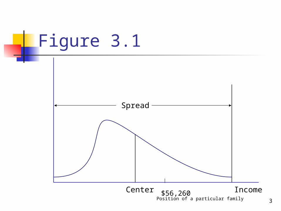
Figure 3.1 Y
-Axi
s
Income Center $56,260
Spread
Position of a particular family
4
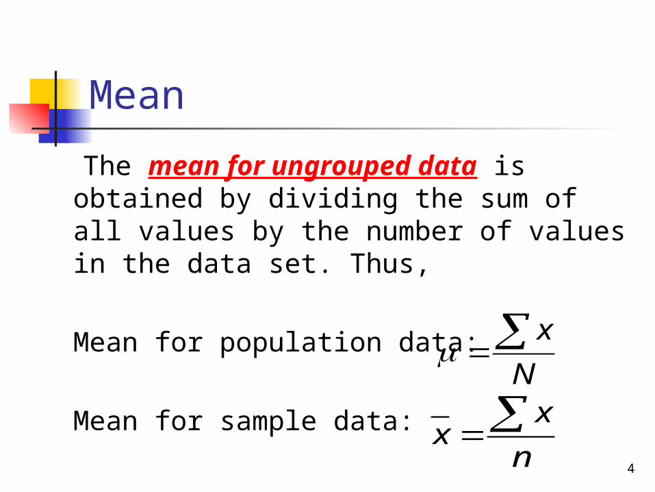
Mean
The mean for ungrouped data is obtained by dividing the sum of all values by the number of values in the data set. Thus,
Mean for population data:
Mean for sample data:
N
x
n
xx

5
Example 3-1
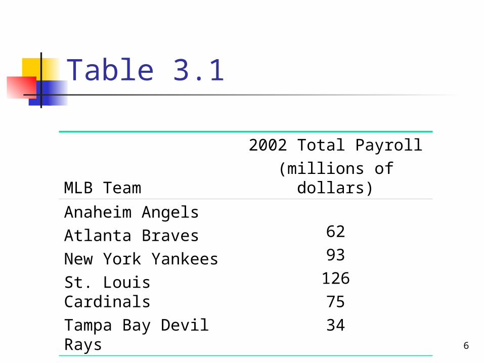
Table 3.1 gives the 2002 total payrolls of five Major League Baseball (MLB) teams.
Find the mean of the 2002 payrolls of these five MLB teams.
6
Table 3.1
MLB Team2002 Total Payroll(millions of dollars)
Anaheim AngelsAtlanta BravesNew York YankeesSt. Louis CardinalsTampa Bay Devil Rays
6293
1267534
7
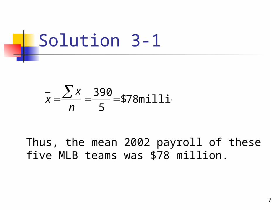
Solution 3-1
million 78$5
390
n
xx
Thus, the mean 2002 payroll of these five MLB teams was $78 million.
8
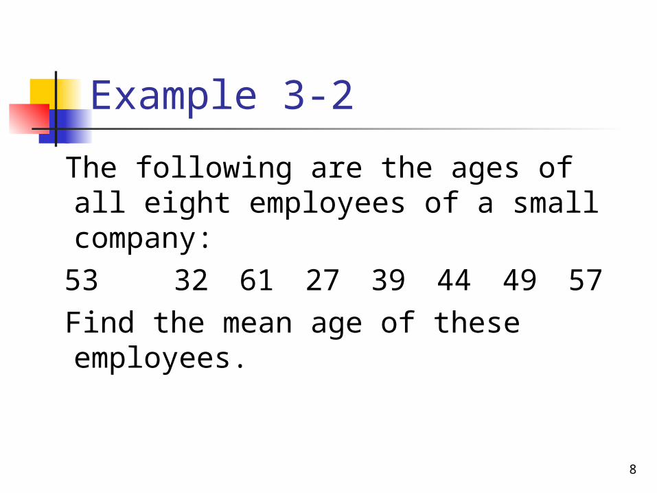
Example 3-2
The following are the ages of all eight employees of a small company:
53 32 61 27 39 44 49 57 Find the mean age of these employees.
9
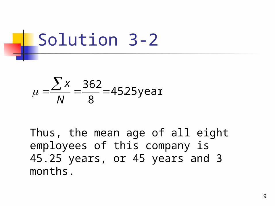
Solution 3-2
years 25.458
362
N
x
Thus, the mean age of all eight employees of this company is 45.25 years, or 45 years and 3 months.
10
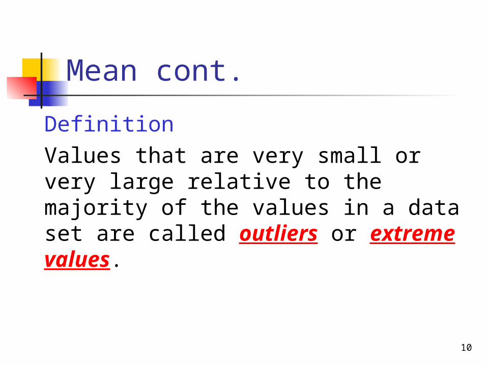
Mean cont.
Definition Values that are very small or very
large relative to the majority of the values in a data set are called outliers or extreme values.
11
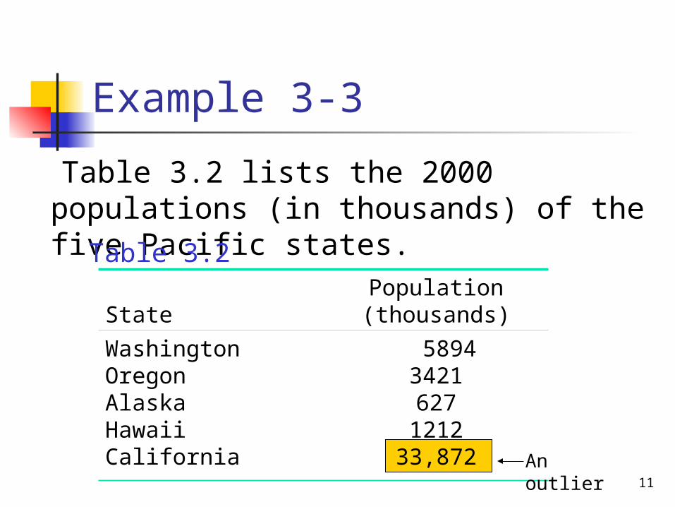
Example 3-3
Table 3.2 lists the 2000 populations (in thousands) of the five Pacific states.
StatePopulation
(thousands)
WashingtonOregonAlaskaHawaiiCalifornia
58943421627
121233,872 An outlier
Table 3.2
12
Example 3-3
Notice that the population of California is very large compared to the populations of the other four states. Hence, it is an outlier. Show how the inclusion of this outlier affects the value of the mean.
13
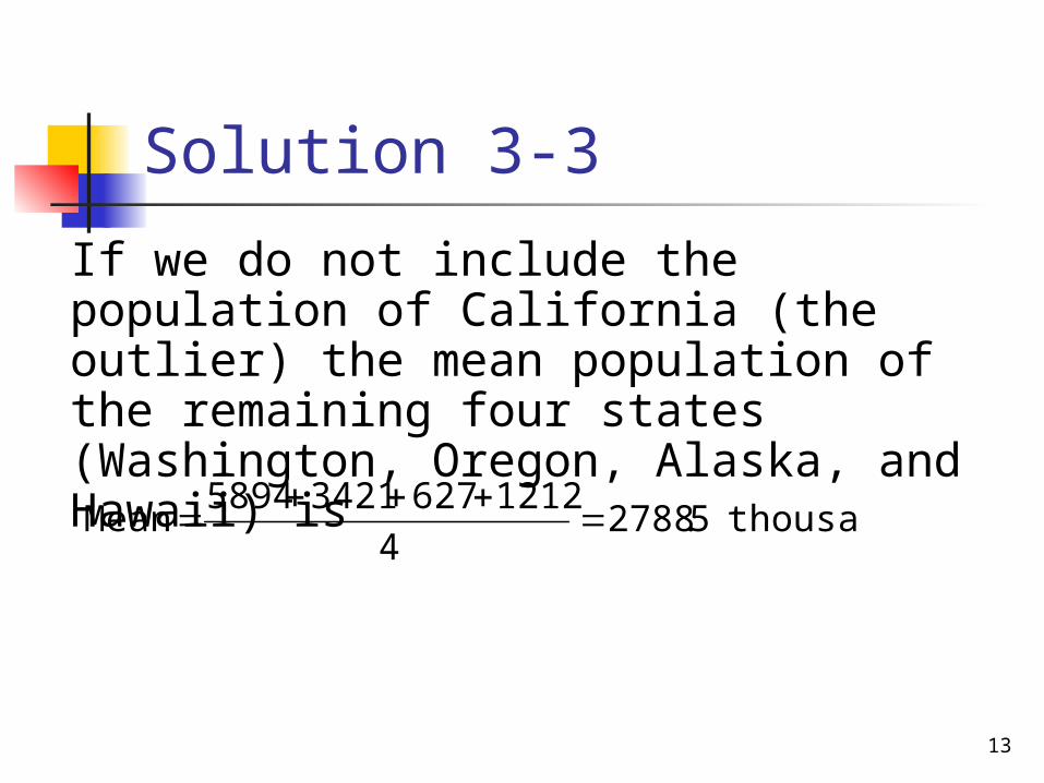
Solution 3-3 If we do not include the population of
California (the outlier) the mean population of the remaining four states (Washington, Oregon, Alaska, and Hawaii) is
thousand5.27884
121262734215894Mean

14
Solution 3-3
Now, to see the impact of the outlier on the value of the mean, we include the population of California and find the mean population of all five Pacific states. This mean is
thousand2.90055
872,33121262734215894Mean

15
Median
Definition The median is the value of the middle
term in a data set that has been ranked in increasing order.
16
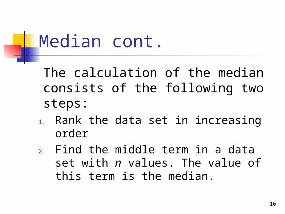
Median cont.
The calculation of the median consists of the following two steps:
1. Rank the data set in increasing order2. Find the middle term in a data set with
n values. The value of this term is the median.
17
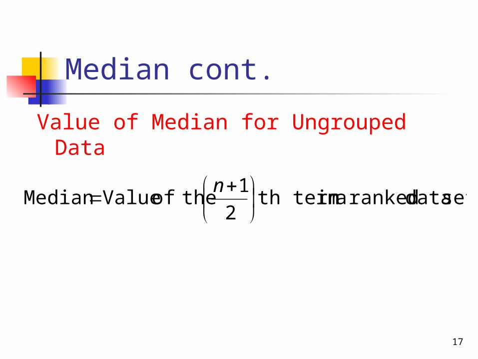
Median cont.
Value of Median for Ungrouped Data
set data ranked ain th term2
1 theof Value Median
n
18
Example 3-4
The following data give the weight lost (in pounds) by a sample of five members of a health club at the end of two months of membership:
10 5 19 8 3 Find the median.

19
Solution 3-4
First, we rank the given data in increasing order as follows:
3 5 8 10 19 There are five observations in the data
set. Consequently, n = 5 and
32
15
2
1 termmiddle theofPosition
n

20
Solution 3-4
Therefore, the median is the value of the third term in the ranked data.
3 5 8 10 19
The median weight loss for this sample of five members of this health club is 8 pounds.
Median
21
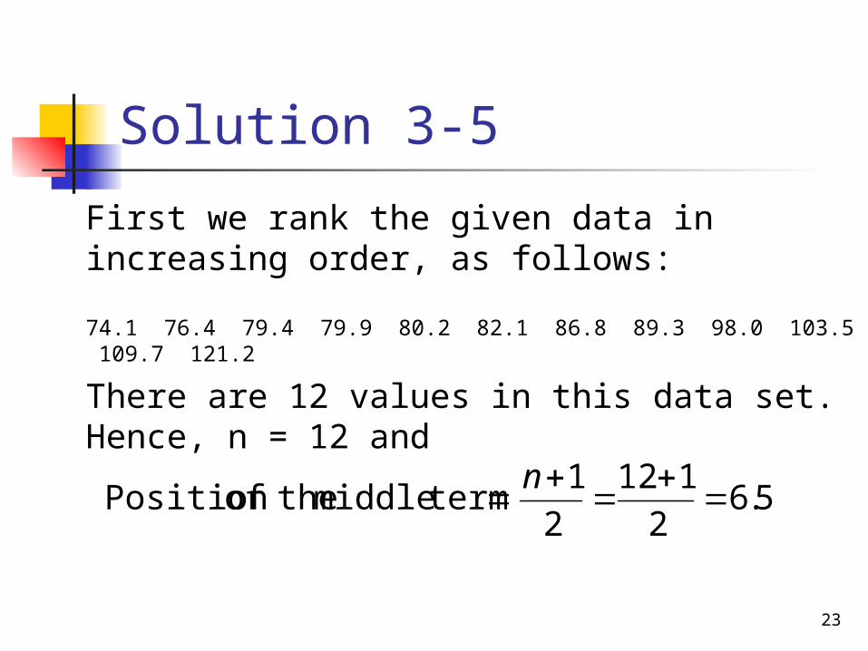
Example 3-5
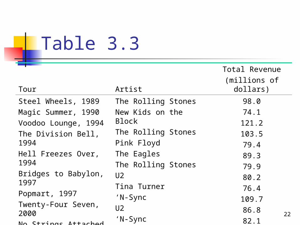
Table 3.3 lists the total revenue for the 12 top-grossing North American concert tours of all time.
Find the median revenue for these data.
22
Table 3.3
Tour ArtistTotal Revenue
(millions of dollars)
Steel Wheels, 1989Magic Summer, 1990Voodoo Lounge, 1994The Division Bell, 1994Hell Freezes Over, 1994Bridges to Babylon, 1997Popmart, 1997Twenty-Four Seven, 2000No Strings Attached, 2000Elevation, 2001Popodyssey, 2001Black and Blue, 2001
The Rolling StonesNew Kids on the BlockThe Rolling StonesPink FloydThe EaglesThe Rolling StonesU2Tina Turner‘N-SyncU2‘N-SyncThe Backstreet Boys
98.074.1121.2103.579.489.379.980.276.4109.786.882.1
23
Solution 3-5 First we rank the given data in increasing
order, as follows:
74.1 76.4 79.4 79.9 80.2 82.1 86.8 89.3 98.0 103.5 109.7 121.2
There are 12 values in this data set. Hence, n = 12 and
5.62
112
2
1 termmiddle theofPosition
n

24
Solution 3-5
Therefore, the median is given by the mean of the sixth and the seventh values in the ranked data.
74.1 76.4 79.4 79.9 80.2 82.1 86.8 89.3 98.0 103.5 109.7 121.2
Thus the median revenue for the 12 top-grossing North American concert tours of all time is $84.45 million.
million 45.84$45.842
8.861.82Median

25
Median cont.
The median gives the center of a histogram, with half the data values to the left of the median and half to the right of the median. The advantage of using the median as a measure of central tendency is that it is not influenced by outliers. Consequently, the median is preferred over the mean as a measure of central tendency for data sets that contain outliers.
26
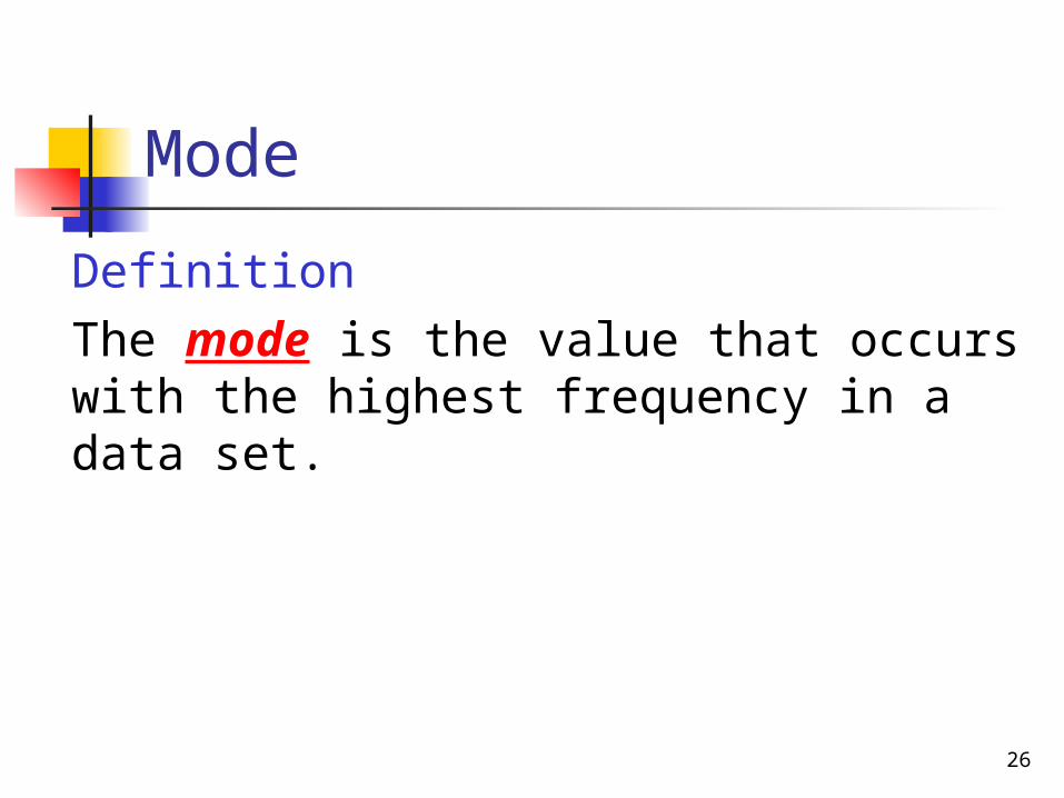
Mode
Definition The mode is the value that occurs with
the highest frequency in a data set.
27
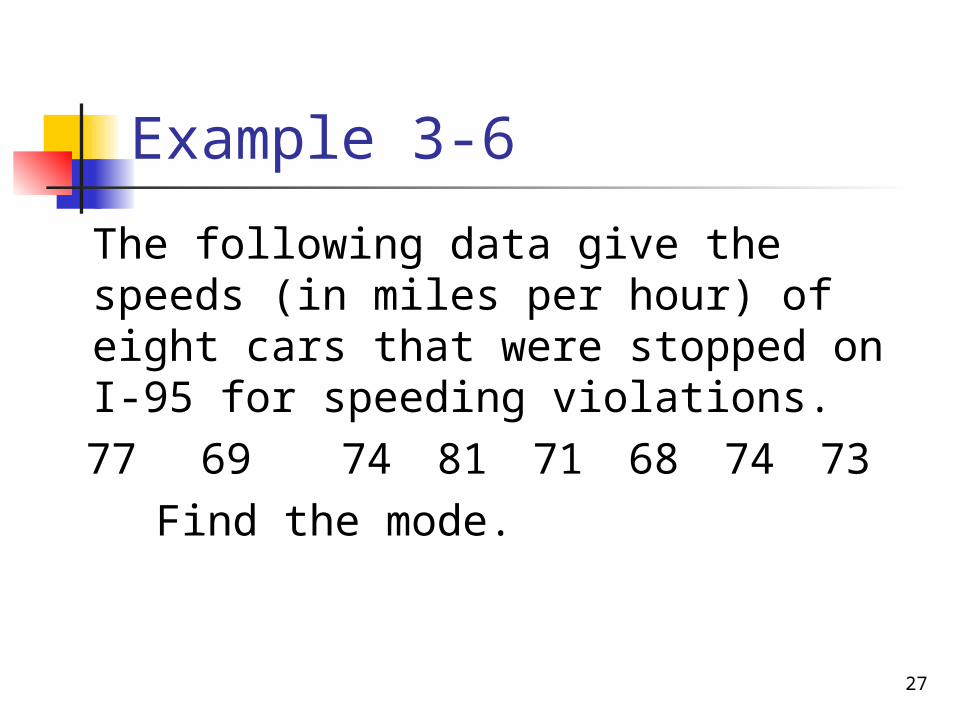
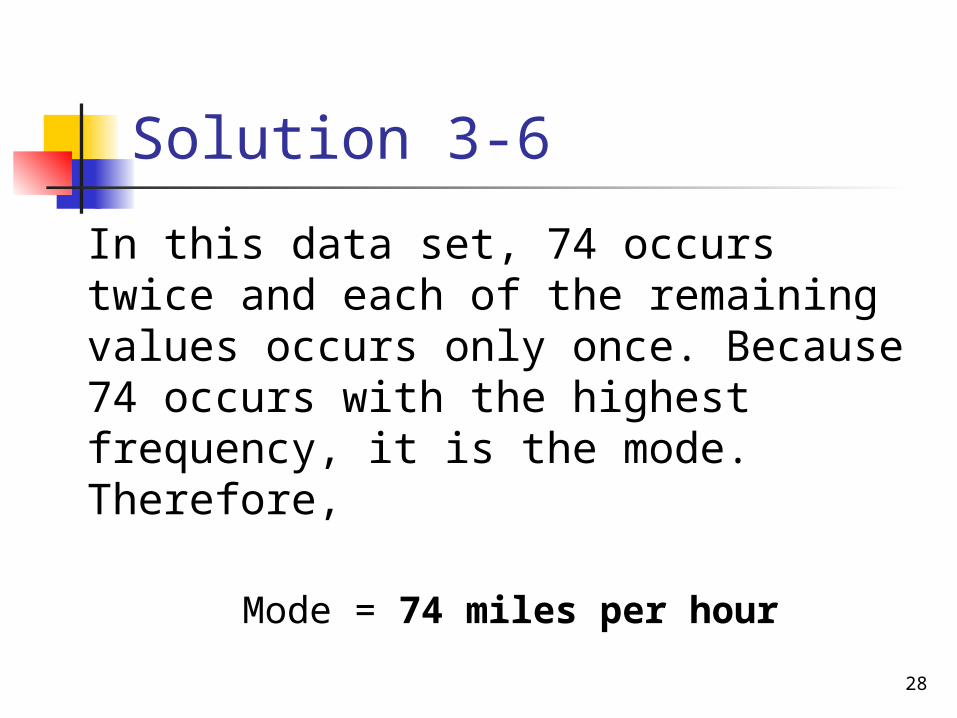
Example 3-6
The following data give the speeds (in miles per hour) of eight cars that were stopped on I-95 for speeding violations.
77 69 74 81 71 68 74 73 Find the mode.
28
Solution 3-6
In this data set, 74 occurs twice and each of the remaining values occurs only once. Because 74 occurs with the highest frequency, it is the mode. Therefore,
Mode = 74 miles per hour

29
Mode cont.
A data set may have none or many modes, whereas it will have only one mean and only one median. The data set with only one mode is
called unimodal. The data set with two modes is called
bimodal. The data set with more than two modes
is called multimodal.

30
Example 3-7
Last year’s incomes of five randomly selected families were $36,150. $95,750, $54,985, $77,490, and $23,740. Find the mode.

31
Solution 3-7
Because each value in this data set occurs only once, this data set contains no mode.
32
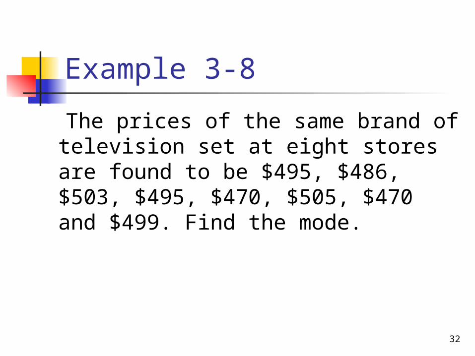
Example 3-8
The prices of the same brand of television set at eight stores are found to be $495, $486, $503, $495, $470, $505, $470 and $499. Find the mode.

33
Solution 3-8
In this data set, each of the two values $495 and $470 occurs twice and each of the remaining values occurs only once.
Therefore, this data set has two modes: $495 and $470.
34
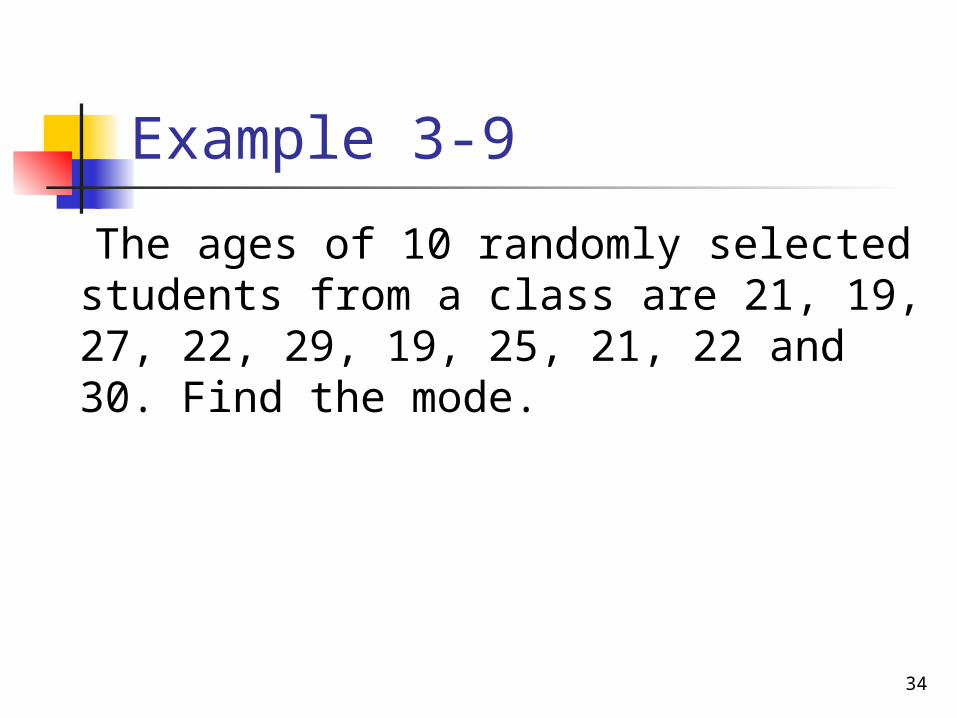
Example 3-9
The ages of 10 randomly selected students from a class are 21, 19, 27, 22, 29, 19, 25, 21, 22 and 30. Find the mode.
35
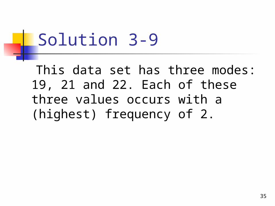
Solution 3-9
This data set has three modes: 19, 21 and 22. Each of these three values occurs with a (highest) frequency of 2.

36
Mode cont.
One advantage of the mode is that it can be calculated for both kinds of data, quantitative and qualitative, whereas the mean and median can be calculated for only quantitative data.
37
Example 3-10
The status of five students who are members of the student senate at a college are senior, sophomore, senior, junior, senior. Find the mode.
38
Solution 3-10
Because senior occurs more frequently than the other categories, it is the mode for this data set.
We cannot calculate the mean and median for this data set.

39
Relationships among the Mean, Median, and Mode
1. For a symmetric histogram and frequency curve with one peak (Figure 3.2), the values of the mean, median, and mode are identical, and they lie at the center of the distribution.

40
Figure 3.2 Mean, median, and mode for a symmetric histogram and frequency curve.
41
Relationships among the Mean, Median, and Mode cont.
2. For a histogram and a frequency curve skewed to the right (Figure 3.3), the value of the mean is the largest, that of the mode is the smallest, and the value of the median lies between these two. Notice that the mode always occurs at the
peak point. The value of the mean is the largest in
this case because it is sensitive to outliers that occur in the right tail. These outliers pull the mean to the right.

42
Figure 3.3 Mean, median, and mode for a histogram and frequency curve skewed to the right.
43
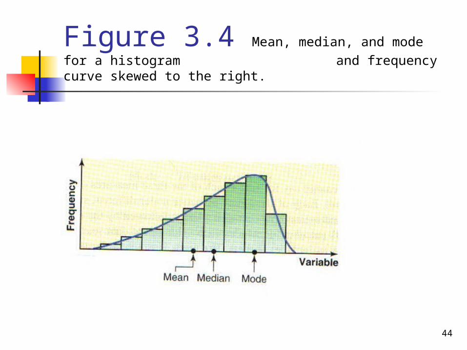
Relationships among the Mean, Median, and Mode cont.
3. If a histogram and a distribution curve are skewed to the left ( Figure 3.4), the value of the mean is the smallest and that of the mode is the largest, with the value of the median lying between these two.
In this case, the outliers in the left tail pull the mean to the left.
44
Figure 3.4 Mean, median, and mode for a histogram and frequency curve skewed to the right.
45
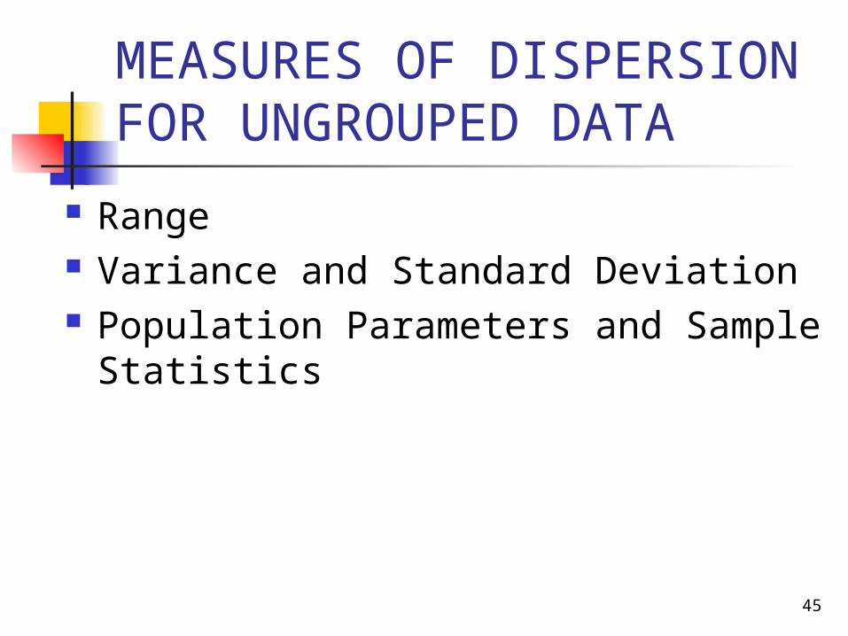
MEASURES OF DISPERSION FOR UNGROUPED DATA
Range Variance and Standard Deviation Population Parameters and Sample
Statistics

46
Range
Finding Range for Ungrouped Data
Range = Largest value – Smallest Value
47
Example 3-11
Table 3.4 gives the total areas in square miles of the four western South-Central states of the United States.
Find the range for this data set.

48
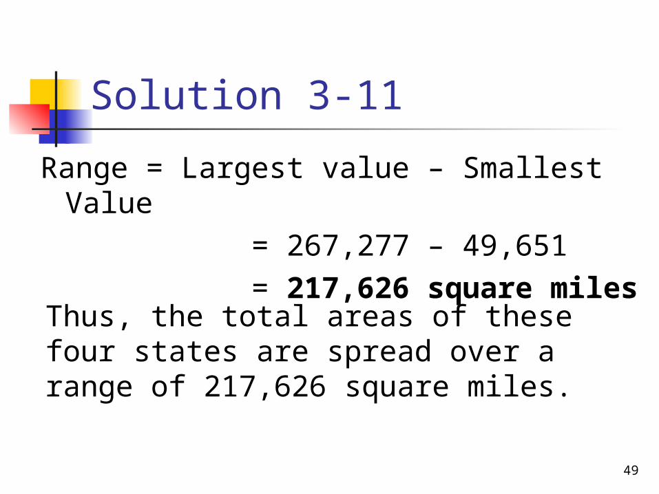
Table 3.4
StateTotal Area
(square miles)
ArkansasLouisianaOklahomaTexas
53,18249,65169,903267,277
49
Solution 3-11
Range = Largest value – Smallest Value = 267,277 – 49,651 = 217,626 square miles Thus, the total areas of these four states are spread over a range of 217,626 square miles.
50
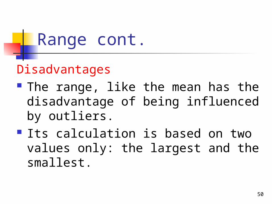
Range cont.
Disadvantages The range, like the mean has the
disadvantage of being influenced by outliers.
Its calculation is based on two values only: the largest and the smallest.
51
Variance and Standard Deviation
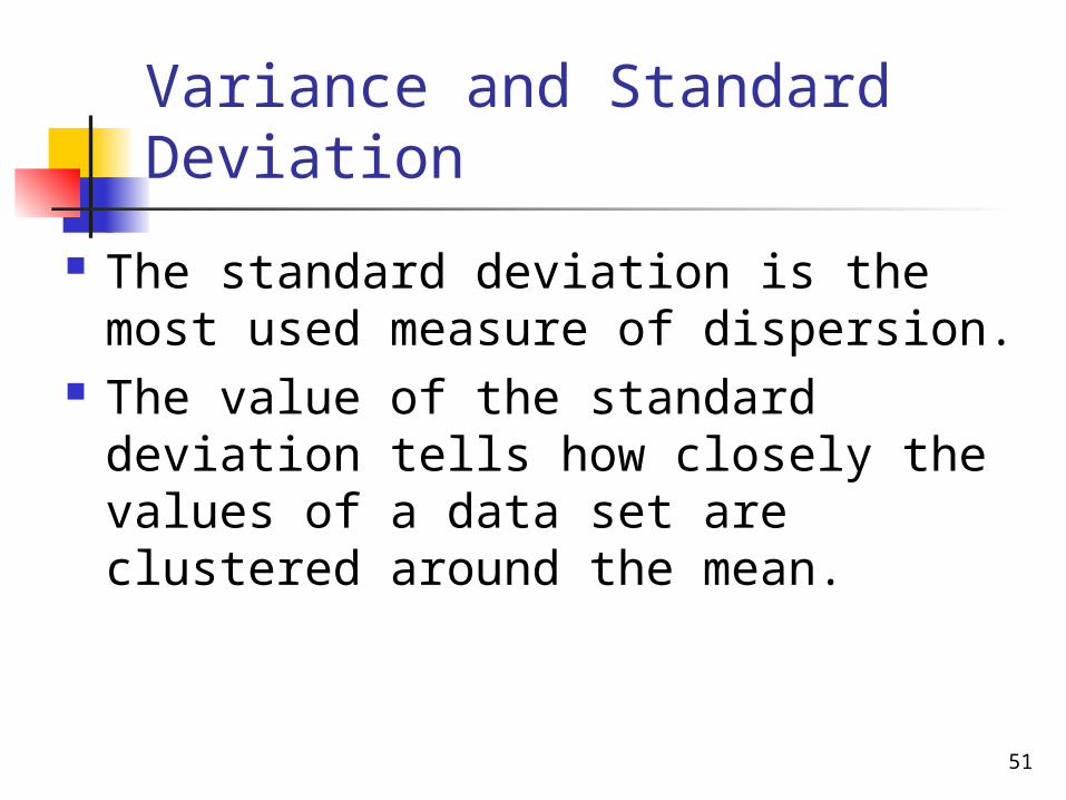
The standard deviation is the most used measure of dispersion.
The value of the standard deviation tells how closely the values of a data set are clustered around the mean.

52
Variance and Standard Deviation cont.
In general, a lower value of the standard deviation for a data set indicates that the values of that data set are spread over a relatively smaller range around the mean.
In contrast, a large value of the standard deviation for a data set indicates that the values of that data set are spread over a relatively large range around the mean.
53
Variance and Standard Deviation cont.
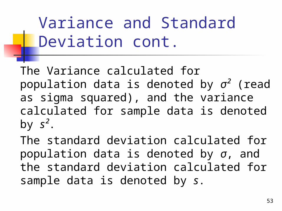
The Variance calculated for population data is denoted by σ² (read as sigma squared), and the variance calculated for sample data is denoted by s².
The standard deviation calculated for population data is denoted by σ, and the standard deviation calculated for sample data is denoted by s.
54
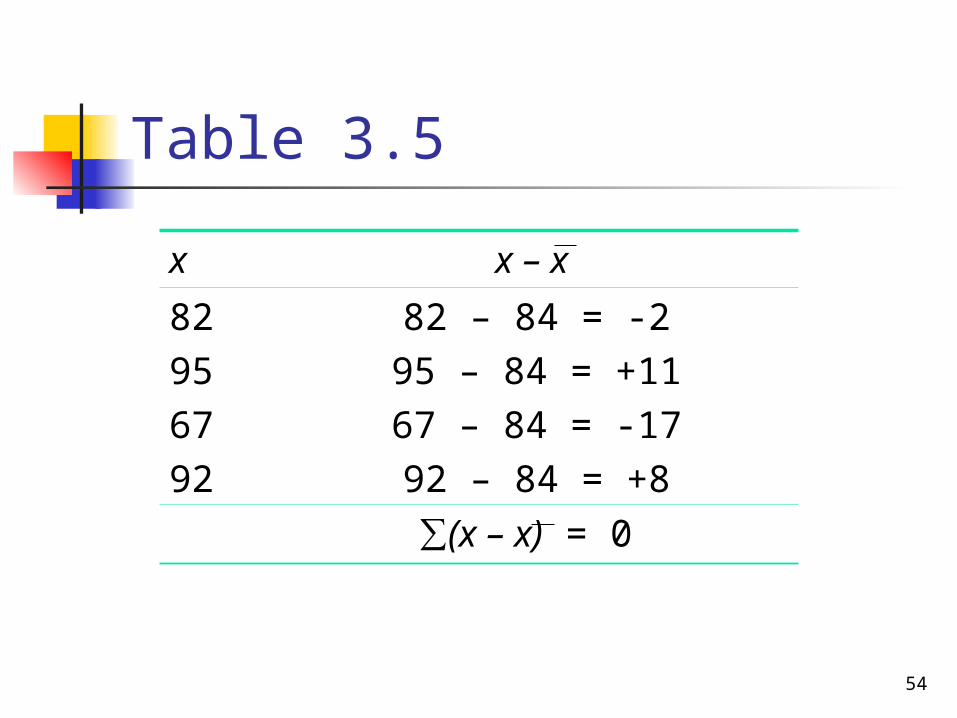
Table 3.5
x x – x
82956792
82 – 84 = -295 – 84 = +1167 – 84 = -1792 – 84 = +8
∑(x – x) = 0
55
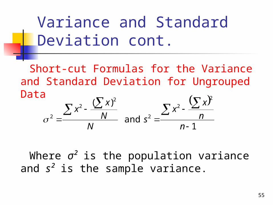
Variance and Standard Deviation cont.
Short-cut Formulas for the Variance and Standard Deviation for Ungrouped Data
Where σ² is the population variance and s² is
the sample variance.
1 and
)(2
2
2
22
2
nn
xx
sN
N
xx
56
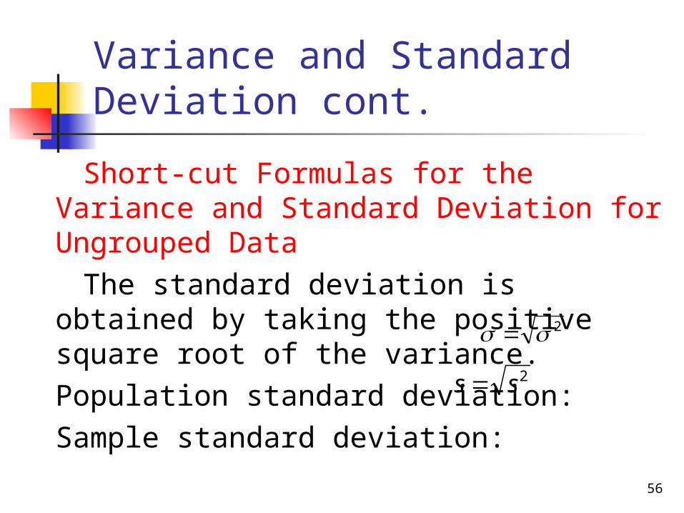
Variance and Standard Deviation cont.
Short-cut Formulas for the Variance and Standard Deviation for Ungrouped Data
The standard deviation is obtained by taking the positive square root of the variance.Population standard deviation:Sample standard deviation:
2ss
2

57
Example 3-12
Refer to data in Table 3.1 on the 2002 total payroll (in millions of dollars) of five MLB teams.
Find the variance and standard deviation of these data

58
Solution 3-12
x x²
62931267534
38448649
15,87656251156
∑x = 390 ∑x² = 35,150
Table 3.6

59
Solution 3-12
498,387,34$387498.3450.1182
50.11824
420,30150,35
155
)390(150,35
1
22
2
2
s
nn
xx
s
Thus, the standard deviation of the 2002 payrolls of these five MLB teams is $34,387,498.
60
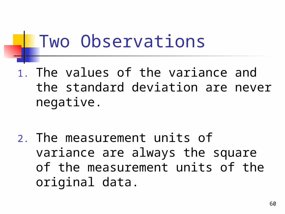
Two Observations
1. The values of the variance and the standard deviation are never negative.
2. The measurement units of variance are always the square of the measurement units of the original data.

61
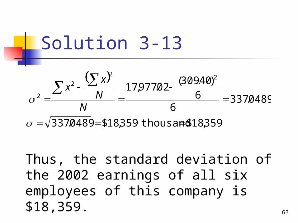
Example 3-13
The following data are the 2002 earnings (in thousands of dollars) before taxes for all six employees of a small company.
48.50 38.40 65.50 22.60 79.80 54.60
Calculate the variance and standard deviation for these data.

62
Solution 3-13
x x²
48.5038.4065.5022.6079.8054.60
2352.251474.564290.25510.766368.042981.16
∑x = 309.40 ∑x² = 17,977.02
Table 3.7
63
Solution 3-13
359,18$ thousand359,18$0489.337
0489.3376
6)40.309(
02.977,17
22
2
2
N
N
xx
Thus, the standard deviation of the 2002 earnings of all six employees of this company is $18,359.
64
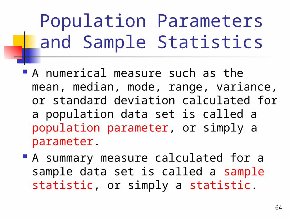
Population Parameters and Sample Statistics
A numerical measure such as the mean, median, mode, range, variance, or standard deviation calculated for a population data set is called a population parameter, or simply a parameter.
A summary measure calculated for a sample data set is called a sample statistic, or simply a statistic.
65
MEAN, VARIANCE AND STANDARD DEVIATION FOR GROUPED DATA
Mean for Grouped Data Variance and Standard Deviation
for Grouped Data
66
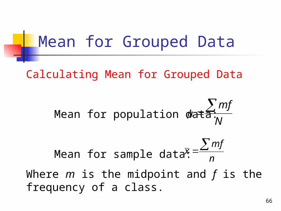
Mean for Grouped Data
N
mf
n
mfx
Calculating Mean for Grouped Data
Mean for population data:
Mean for sample data:
Where m is the midpoint and f is the frequency of a class.
67
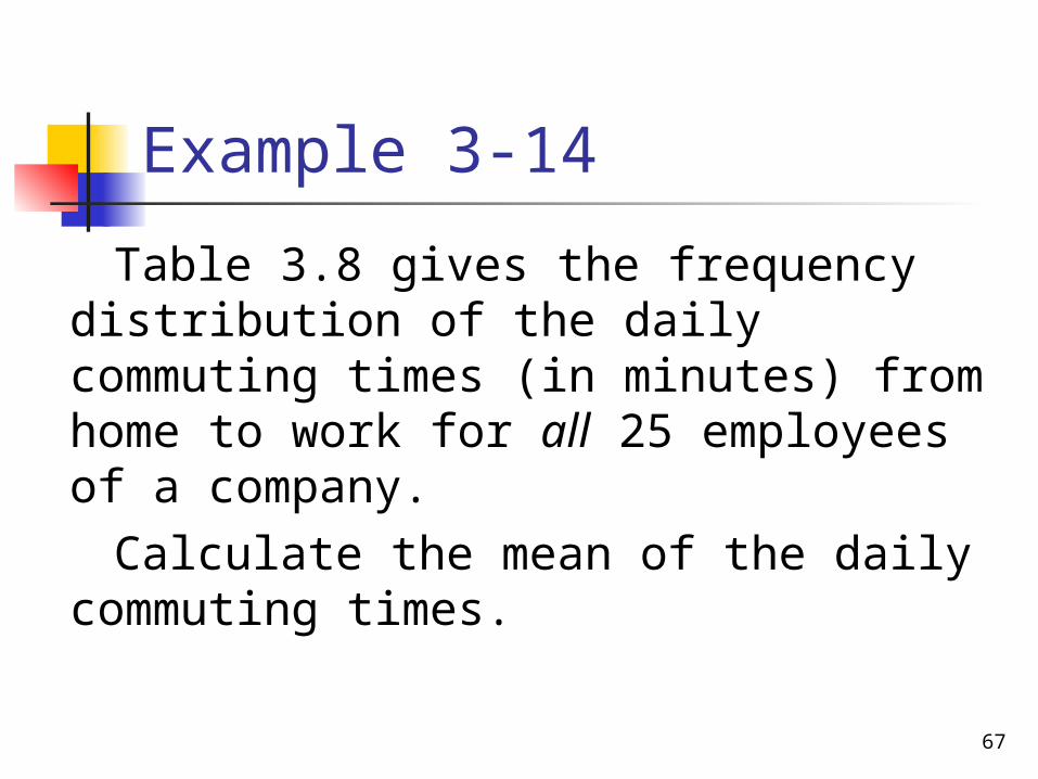
Example 3-14
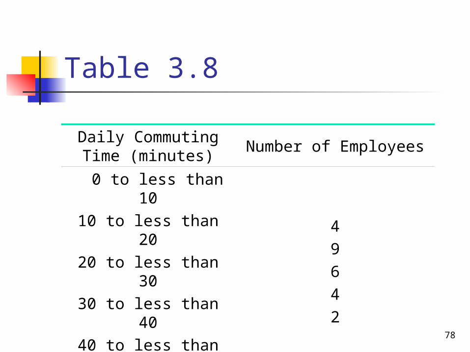
Table 3.8 gives the frequency distribution of the daily commuting times (in minutes) from home to work for all 25 employees of a company.
Calculate the mean of the daily commuting times.

68
Table 3.8
Daily Commuting Time (minutes)
Number of Employees
0 to less than 1010 to less than 2020 to less than 3030 to less than 4040 to less than 50
49642
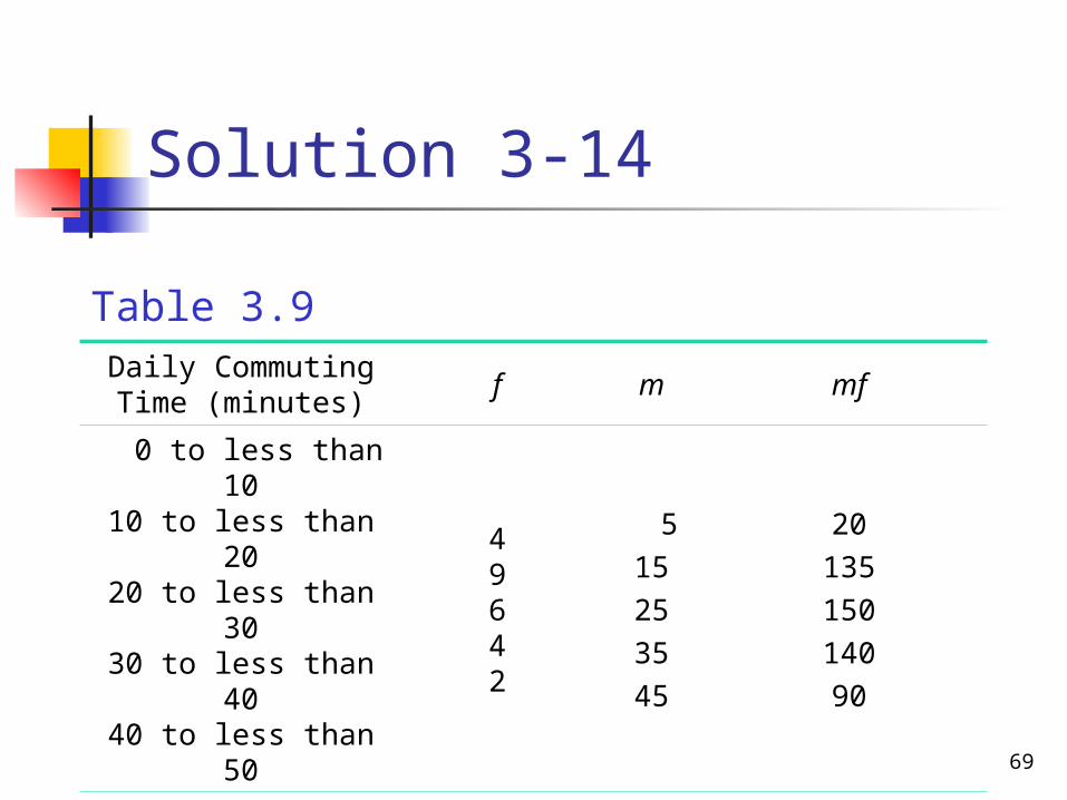
69
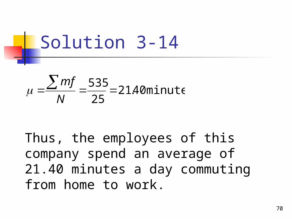
Solution 3-14
Daily Commuting Time (minutes)
f m mf
0 to less than 1010 to less than 2020 to less than 3030 to less than 4040 to less than 50
49642
515253545
2013515014090
N = 25 ∑mf = 535
Table 3.9
70
Solution 3-14
minutes 40.2125
535
N
mf
Thus, the employees of this company spend an average of 21.40 minutes a day commuting from home to work.
71
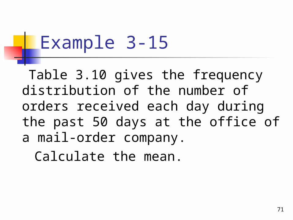
Example 3-15
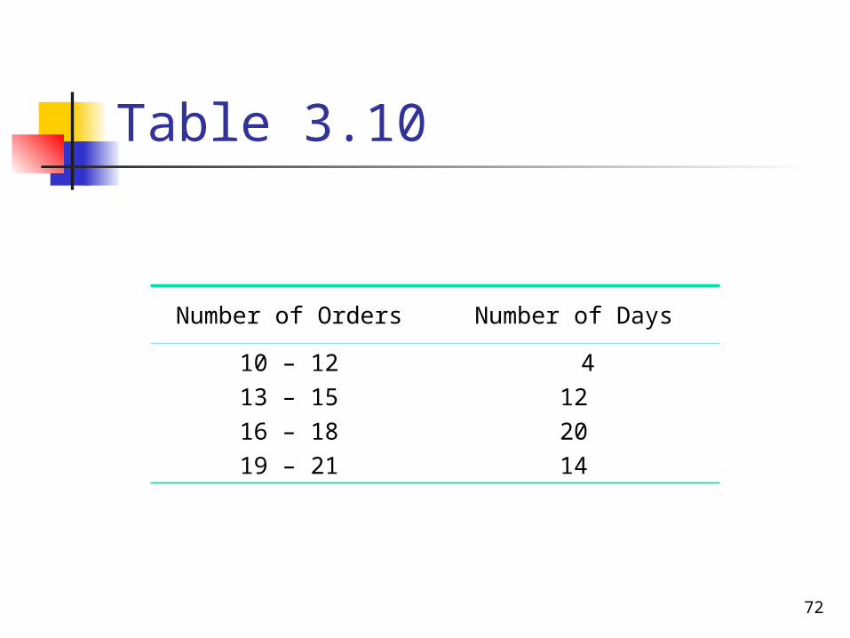
Table 3.10 gives the frequency distribution of the number of orders received each day during the past 50 days at the office of a mail-order company.
Calculate the mean.
72
Table 3.10
Number of Orders Number of Days
10 – 12
13 – 15
16 – 18
19 – 21
4
12
20
14
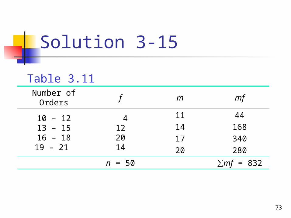
73
Solution 3-15
Number of Orders
f m mf
10 – 1213 – 1516 – 1819 – 21
4122014
11141720
44168340280
n = 50 ∑mf = 832
Table 3.11
74
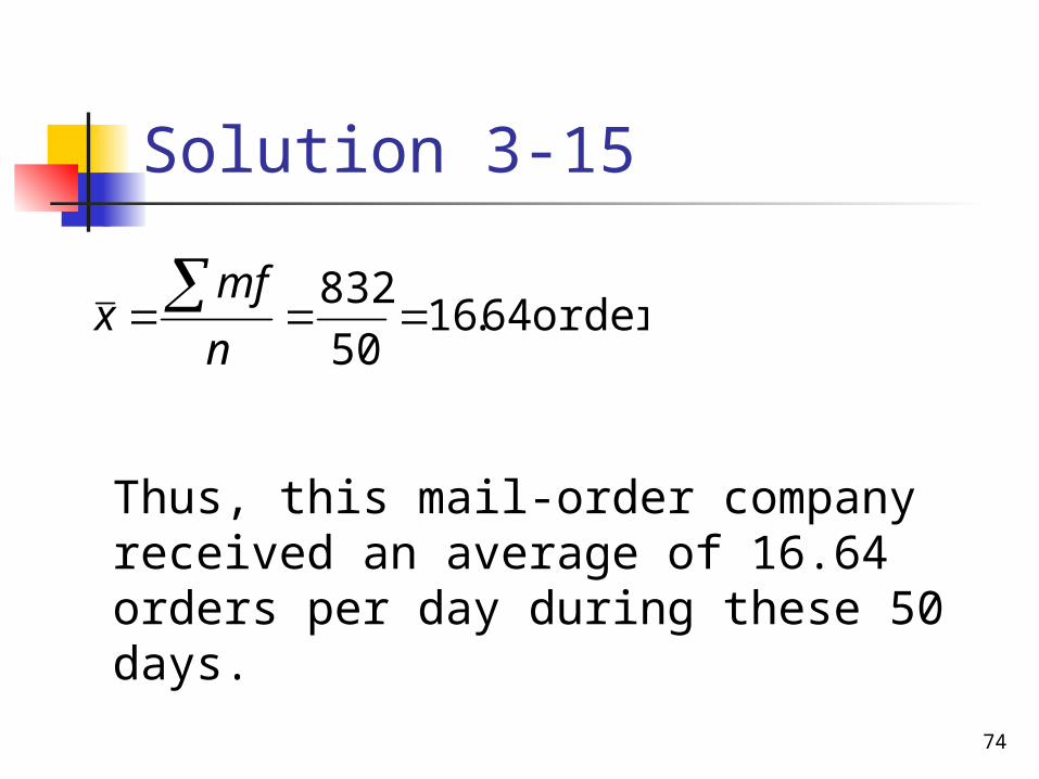
Solution 3-15
orders 64.1650
832
n
mfx
Thus, this mail-order company received an average of 16.64 orders per day during these 50 days.
75
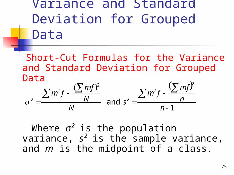
Variance and Standard Deviation for Grouped Data
Short-Cut Formulas for the Variance and Standard Deviation for Grouped Data
Where σ² is the population variance, s² is the sample variance, and m is the midpoint of a class.
1 and
)(2
2
2
22
2
nn
mffm
sN
N
mffm

76
Variance and Standard Deviation for Grouped Data cont.
Short-cut Formulas for the Variance and Standard Deviation for Grouped Data
The standard deviation is obtained by taking the positive square root of the variance.Population standard deviation:Sample standard deviation:
2ss
2

77
Example 3-16
Table 3.8 gives the frequency distribution of the daily commuting times (in minutes) from home to work for all 25 employees of a company.
Calculate the variance and standard deviation.
78
Table 3.8
Daily Commuting Time (minutes)
Number of Employees
0 to less than 1010 to less than 2020 to less than 3030 to less than 4040 to less than 50
49642
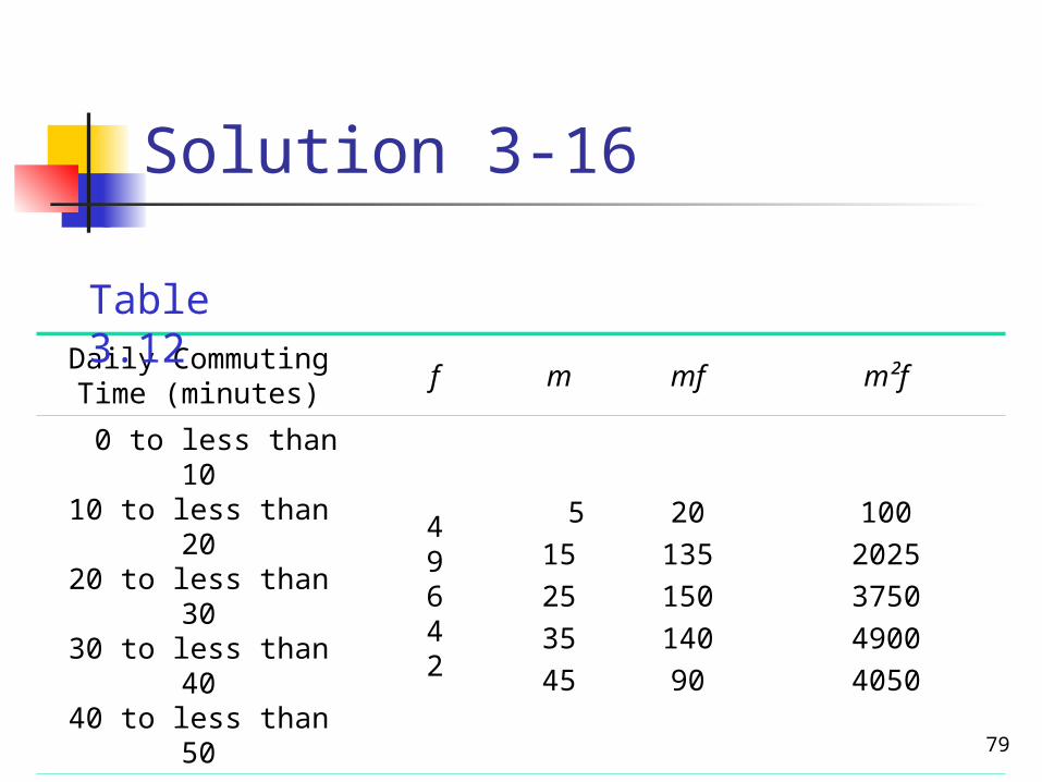
79
Solution 3-16
Daily Commuting Time (minutes)
f m mf m²f
0 to less than 1010 to less than 2020 to less than 3030 to less than 4040 to less than 50
49642
515253545
2013515014090
1002025375049004050
N = 25∑mf = 535
∑m²f = 14,825
Table 3.12

80
Solution 3-16
minutes 62.1104.135
04.13525
3376
2525
)535(825,14
)(
2
222
2
N
N
mffm
Thus, the standard deviation of the daily commuting times for these employees is 11.62 minutes.
Hence, the standard deviation is
81
Example 3-17
Table 3.10 gives the frequency distribution of the number of orders received each day during the past 50 days at the office of a mail-order company.
Calculate the variance and standard deviation.

82
Table 3.10
Number of Orders f
10 – 1213 – 1516 – 1819 – 21
4122014
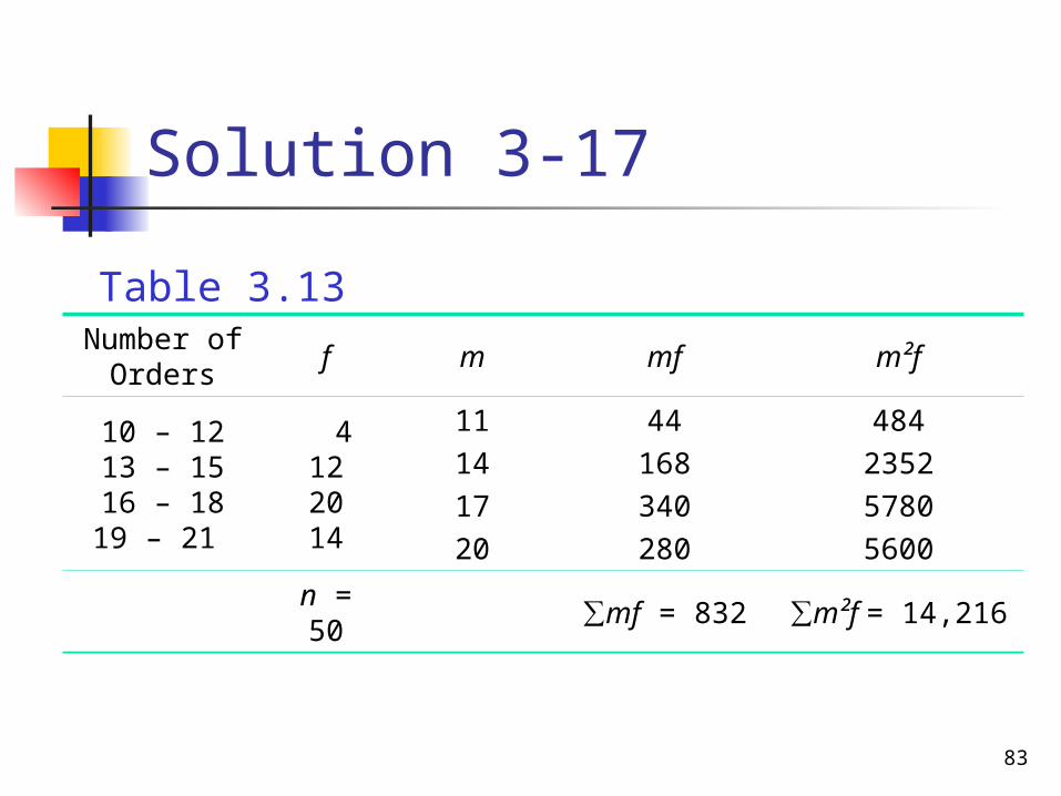
83
Solution 3-17
Number of Orders
f m mf m²f
10 – 1213 – 1516 – 1819 – 21
4122014
11141720
44168340280
484235257805600
n = 50 ∑mf = 832 ∑m²f = 14,216
Table 3.13

84
Solution 3-17
orders 75.25820.7
5820.7150
50)832(
216,14
1
)(
2
222
2
ss
nn
mffm
s
Thus, the standard deviation of the number of orders received at the office of this mail-order company during the past 50 days in 2.75.
Hence, the standard deviation is
85
USE OF STANDARD DEVIATION
Chebyshev’s Theorem Empirical Rule

86
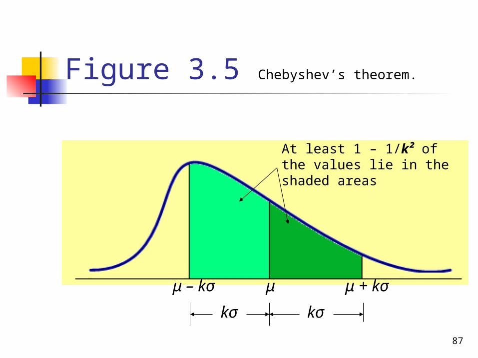
Chebyshev’s Theorem
Definition For any number k greater than 1, at
least (1 – 1/k²) of the data values lie within k standard deviations of the mean.
87
Figure 3.5 Chebyshev’s theorem.
μ – kσ
kσ
μ
kσ
μ + kσ
At least 1 – 1/k² of the values lie in the shaded areas
88
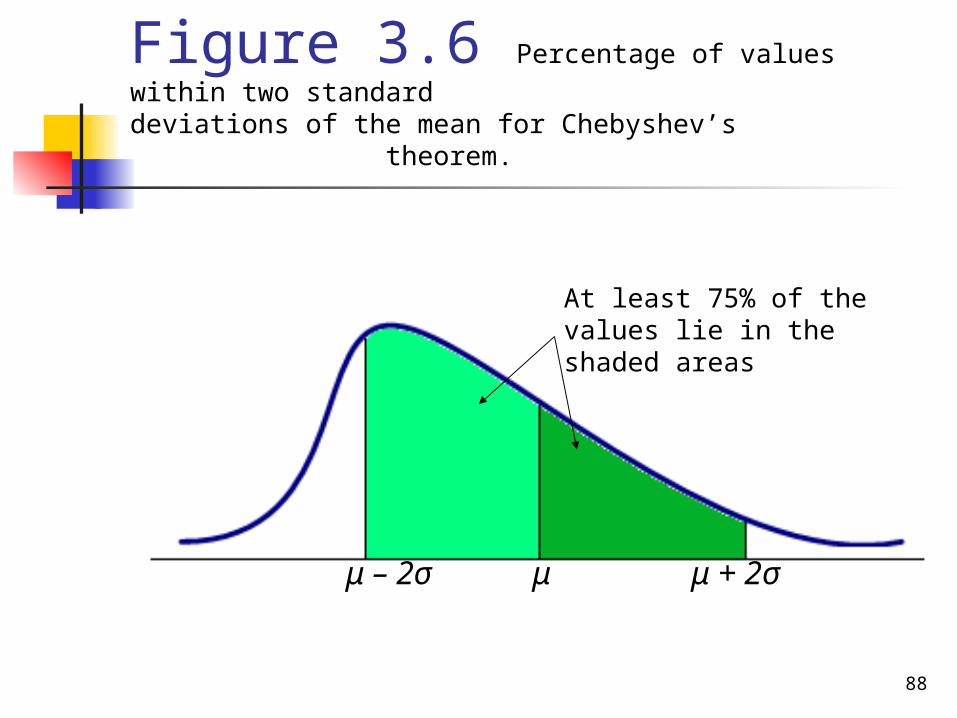
Figure 3.6 Percentage of values within two standard deviations of the mean for Chebyshev’s theorem.
μ – 2σ μ μ + 2σ
At least 75% of the values lie in the shaded areas
89
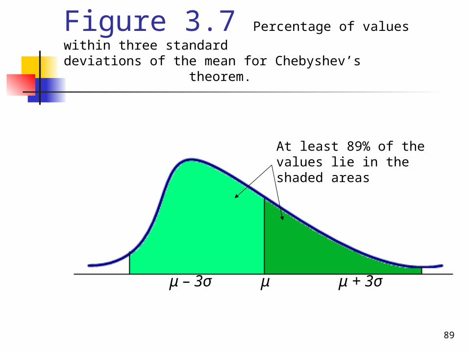
Figure 3.7 Percentage of values within three standard deviations of the mean for Chebyshev’s theorem.
μ – 3σ μ μ + 3σ
At least 89% of the values lie in the shaded areas
90
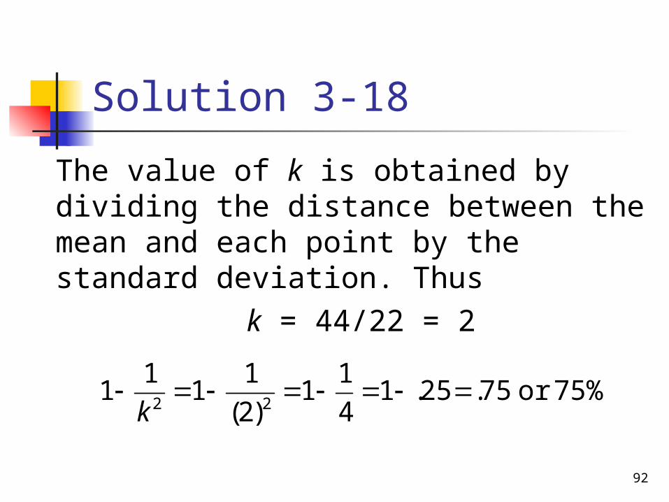
Example 3-18
The average systolic blood pressure for 4000 women who were screened for high blood pressure was found to be 187 with a standard deviation of 22. Using Chebyshev’s theorem, find at least what percentage of women in this group have a systolic blood pressure between 143 and 231.

91
Solution 3-18
Let μ and σ be the mean and the standard deviation, respectively, of the systolic blood pressures of these women.
μ = 187 and σ = 22
143 - 187 = -44 231 - 187 = 44
μ = 187 143 231
92
Solution 3-18
The value of k is obtained by dividing the distance between the mean and each point by the standard deviation. Thus
k = 44/22 = 2
75%or 75.25.14
11
)2(
11
11
22
k
93
Solution 3-18
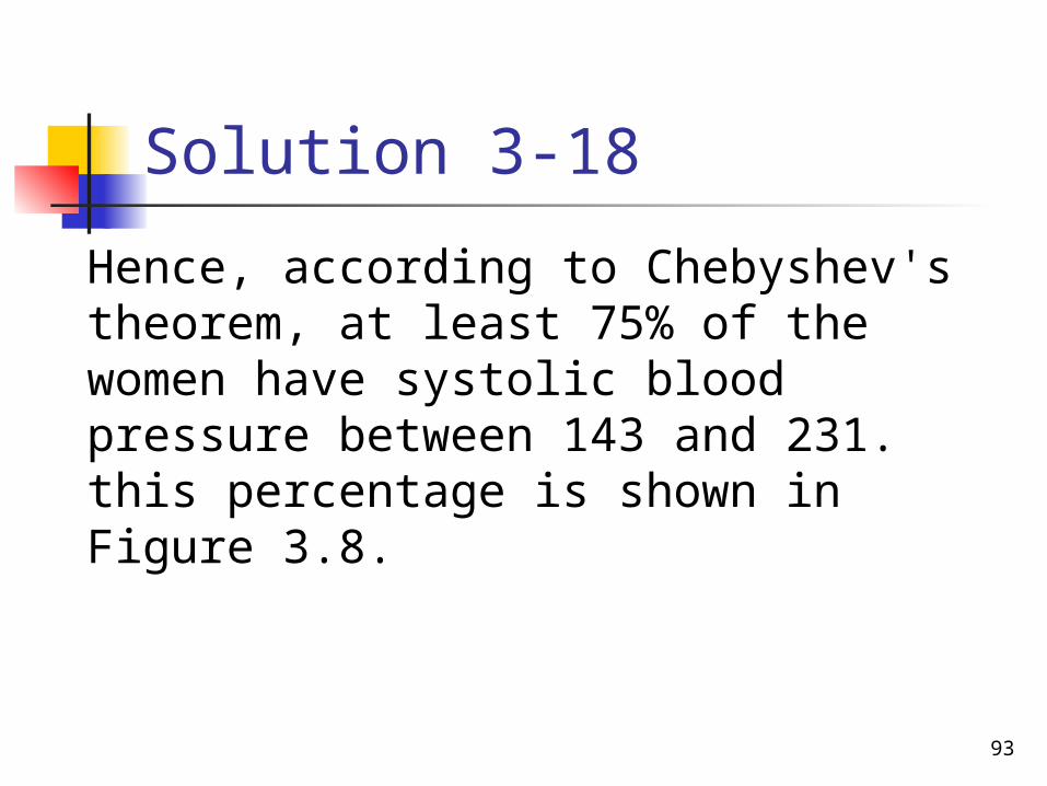
Hence, according to Chebyshev's theorem, at least 75% of the women have systolic blood pressure between 143 and 231. this percentage is shown in Figure 3.8.
94
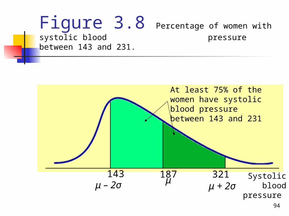
Figure 3.8 Percentage of women with systolic blood pressure between 143 and 231.
143 μ – 2σ
187μ
321 μ + 2σ
At least 75% of the women have systolic blood pressure between 143 and 231
Systolic blood
pressure
95
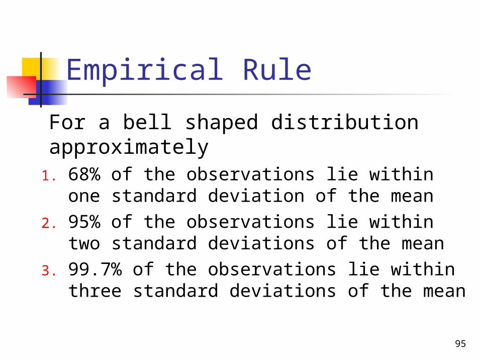
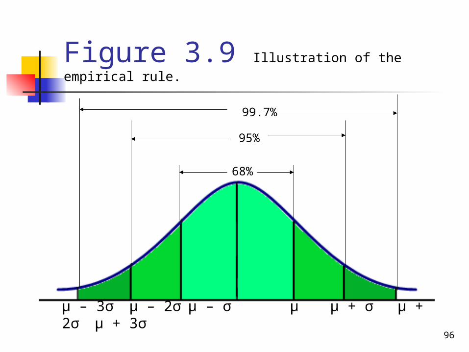
Empirical Rule
For a bell shaped distribution approximately
1. 68% of the observations lie within one standard deviation of the mean
2. 95% of the observations lie within two standard deviations of the mean
3. 99.7% of the observations lie within three standard deviations of the mean
96
Figure 3.9 Illustration of the empirical rule.
μ – 3σ μ – 2σμ – σ μ μ + σ μ + 2σ μ + 3σ
68%
99.7%
95%

97
Example 3-19
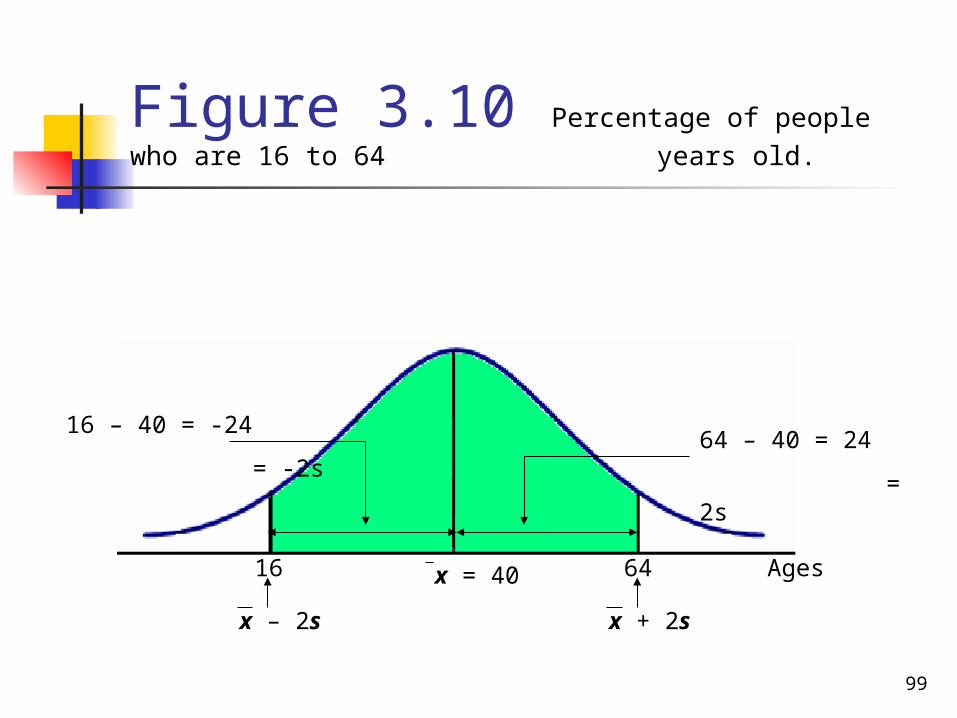
The age distribution of a sample of 5000 persons is bell-shaped with a mean of 40 years and a standard deviation of 12 years. Determine the approximate percentage of people who are 16 to 64 years old.

98
Solution 3-19 From the given information, for this distribution, x = 40 and s = 12 years
Each of the two points, 16 and 64, is 24 units away from the mean.
Because the area within two standard deviations of the mean is approximately 95% for a bell-shaped curve, approximately 95% of the people in the sample are 16 to 64 years old.
99
Figure 3.10 Percentage of people who are 16 to 64 years old.
16 64 x = 40
x – 2s x + 2s
16 – 40 = -24
= -2s64 – 40 = 24
= 2s
Ages
100
MEASURES OF POSITION
Quartiles and Interquartile Range Percentiles and Percentile Rank

101
Quartiles and Interquartile Range
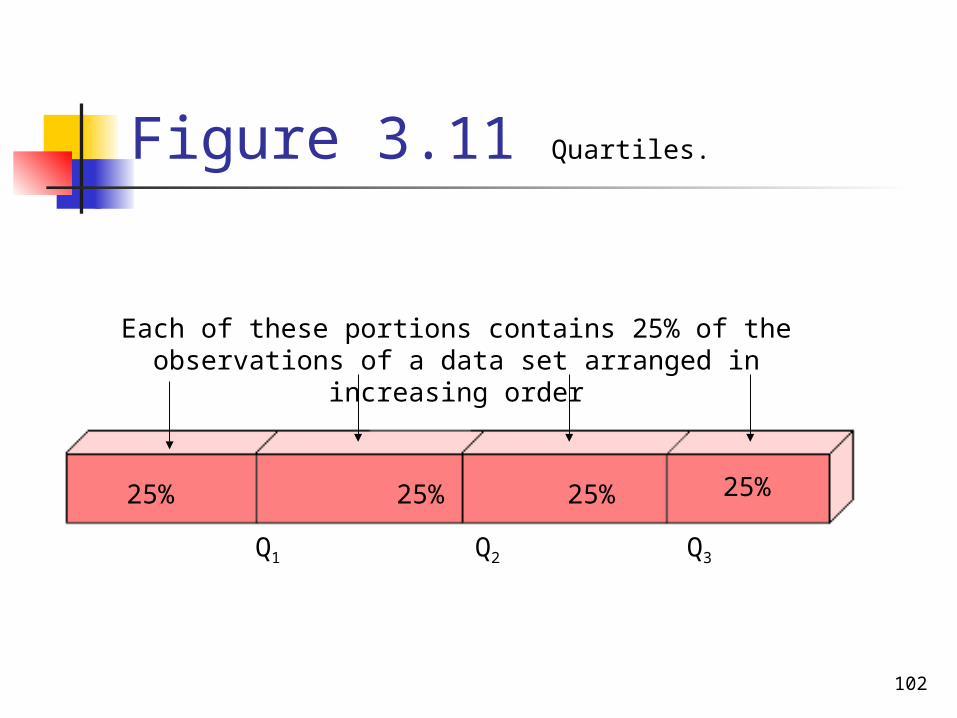
Definition Quartiles are three summery measures that
divide a ranked data set into four equal parts. The second quartile is the same as the median of a data set. The first quartile is the value of the middle term among the observations that are less than the median, and the third quartile is the value of the middle term among the observations that are greater than the median.
102
Figure 3.11 Quartiles.
25% 25% 25% 25%
Each of these portions contains 25% of the observations of a data set arranged in increasing order
Q1 Q2 Q3

103
Quartiles and Interquartile Range cont.
Calculating Interquartile Range The difference between the third and
first quartiles gives the interquartile range; that is, IQR = Interquartile range = Q3 – Q1
104
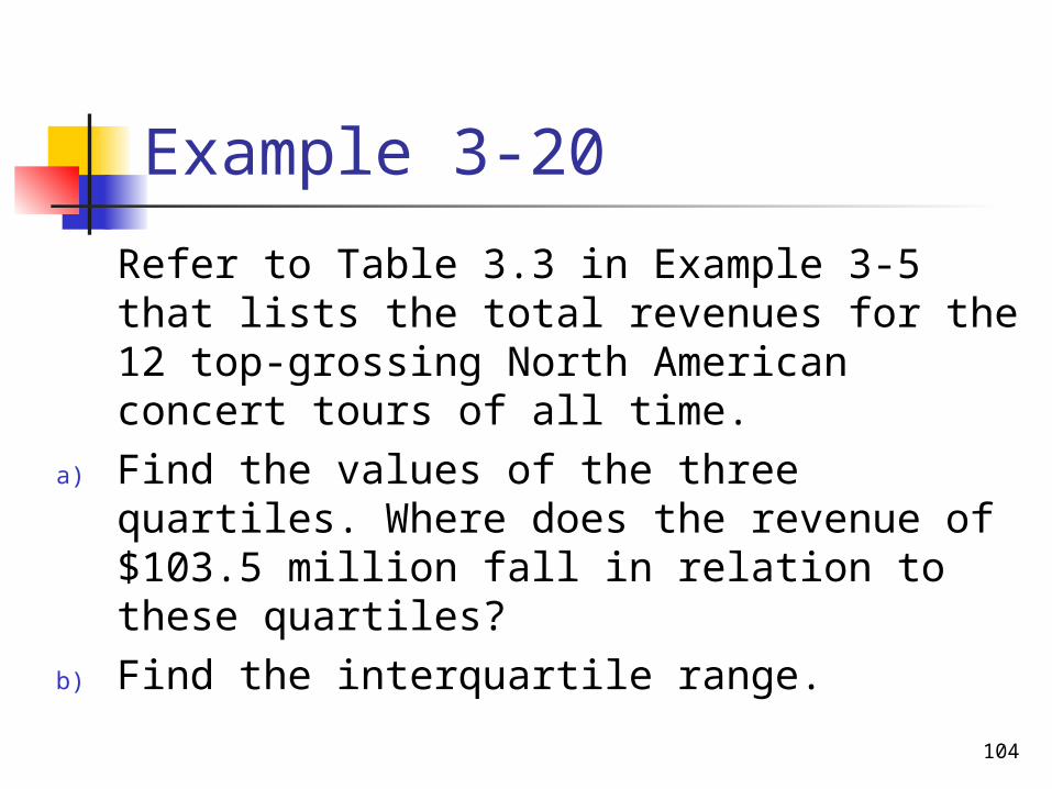
Example 3-20
Refer to Table 3.3 in Example 3-5 that lists the total revenues for the 12 top-grossing North American concert tours of all time.
a) Find the values of the three quartiles. Where does the revenue of $103.5 million fall in relation to these quartiles?
b) Find the interquartile range.
105
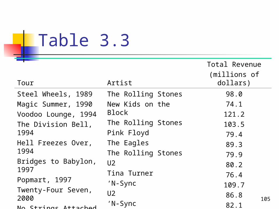
Table 3.3
Tour ArtistTotal Revenue
(millions of dollars)
Steel Wheels, 1989Magic Summer, 1990Voodoo Lounge, 1994The Division Bell, 1994Hell Freezes Over, 1994Bridges to Babylon, 1997Popmart, 1997Twenty-Four Seven, 2000No Strings Attached, 2000Elevation, 2001Popodyssey, 2001Black and Blue, 2001
The Rolling StonesNew Kids on the BlockThe Rolling StonesPink FloydThe EaglesThe Rolling StonesU2Tina Turner‘N-SyncU2‘N-SyncThe Backstreet Boys
98.074.1121.2103.579.489.379.980.276.4109.786.882.1
106
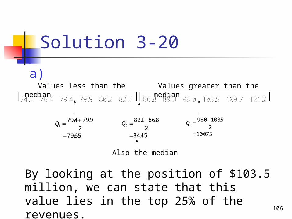
Solution 3-20
74.1 76.4 79.4 79.9 80.2 82.1 86.8 89.3 98.0 103.5 109.7 121.2
65.79 2
9.794.791
Q
45.84 2
8.861.822
Q
75.100 2
5.1030.983
Q
Also the median
Values less than the median Values greater than the median
a)
By looking at the position of $103.5 million, we can state that this value lies in the top 25% of the revenues.

107
Solution 3-20
b)IQR = Interquartile range = Q3 – Q1
= 100.75 – 79.65
= $21.10 million

108
Example 3-21
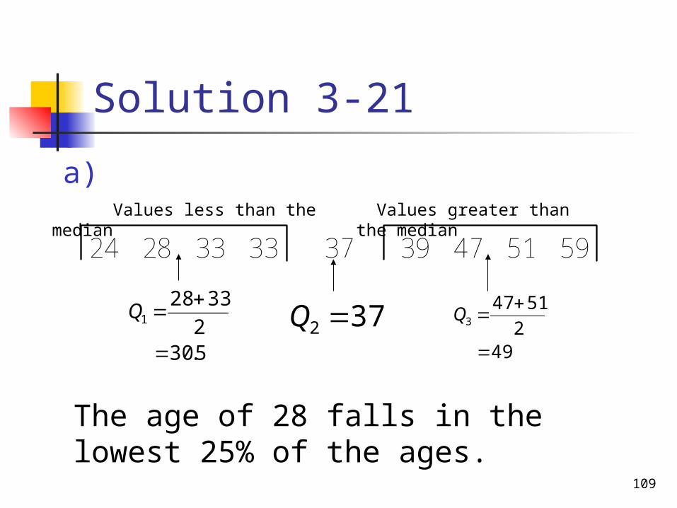
The following are the ages of nine employees of an insurance company:
47 28 39 51 33 37 59 24 33a) Find the values of the three quartiles.
Where does the age of 28 fall in relation to the ages of the employees?
b) Find the interquartile range.
109
Solution 3-21
a)
24 28 33 33 37 39 47 51 59
49 2
51473
Q
5.30 2
33281
Q 372 Q
Values less than the median Values greater than the median
The age of 28 falls in the lowest 25% of the ages.
110
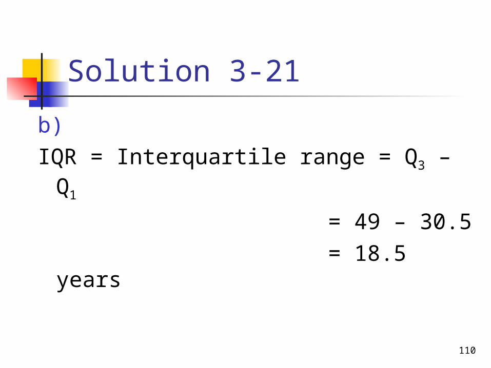
Solution 3-21
b)IQR = Interquartile range = Q3 – Q1
= 49 – 30.5 = 18.5 years

111
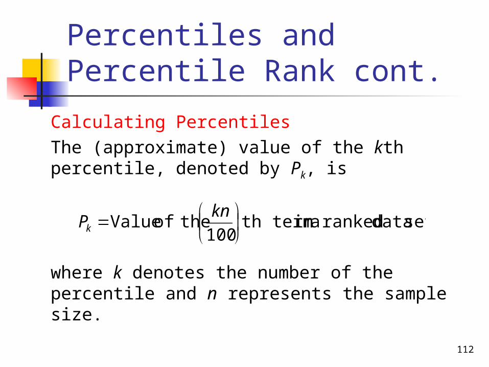
Percentiles and Percentile Rank
Figure 3.12 Percentiles.
1% 1%1% 1% 1% 1%
P1 P2 P3 P97 P98 P99
Each of these portions contains 1% of the observations of a data set arranged in increasing
order
112
Percentiles and Percentile Rank cont.
Calculating Percentiles The (approximate) value of the kth
percentile, denoted by Pk, is
where k denotes the number of the percentile and n represents the sample size.
set data ranked ain th term100
theof Value
knPk

113
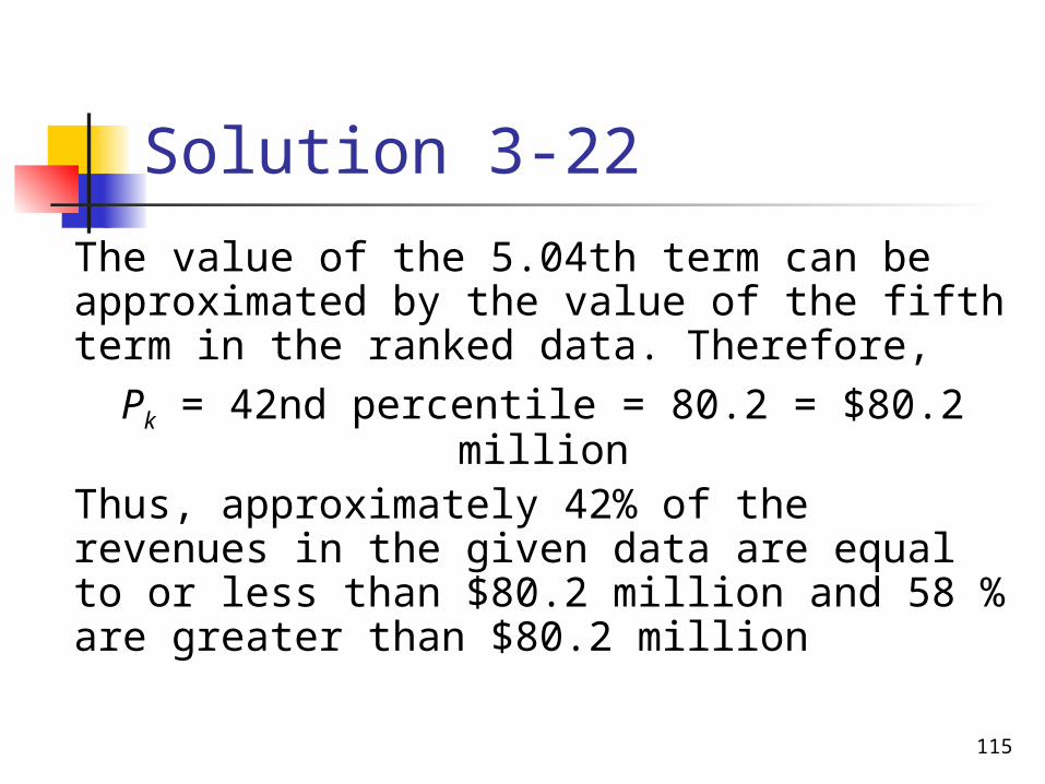
Example 3-22
Refer to the data on revenues for the 12 top-grossing North American concert tours of all time given in Example 3-20. Find the value of the 42nd percentile. Give a brief interpretation of the 42nd percentile.

114
Solution 3-22 The data arranged in increasing order as
follows:
The position of the 42nd percentile is
74.1 76.4 79.4 79.9 80.2 82.1 86.8 89.3 98.0 103.5 109.7 121.2
th term04.5100
)12)(42(
100
kn
115
Solution 3-22 The value of the 5.04th term can be
approximated by the value of the fifth term in the ranked data. Therefore, Pk = 42nd percentile = 80.2 = $80.2
million Thus, approximately 42% of the
revenues in the given data are equal to or less than $80.2 million and 58 % are greater than $80.2 million

116
Percentiles and Percentile Rank cont.
Finding Percentile Rank of a Value
100set data in the valuesofnumber Total
than less valuesofNumber ofrank Percentile i
i
xx
117
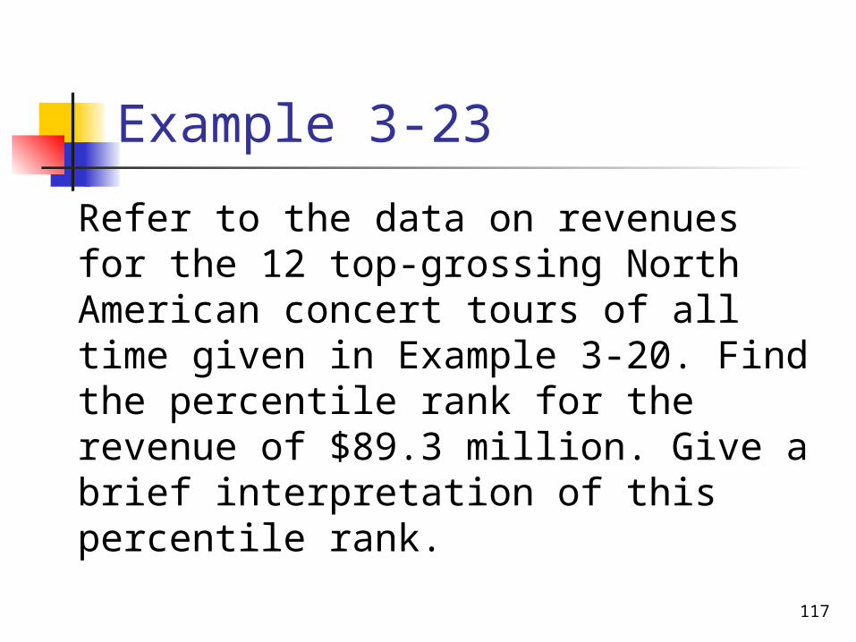
Example 3-23
Refer to the data on revenues for the 12 top-grossing North American concert tours of all time given in Example 3-20. Find the percentile rank for the revenue of $89.3 million. Give a brief interpretation of this percentile rank.

118
Solution 3-23 The data on revenues arranged in increasing
order is as follows:
In this data set, 7 of the 12 revenues are less than $89.3 million. Hence,
74.1 76.4 79.4 79.9 80.2 82.1 86.8 89.3 98.0 103.5 109.7 121.2
%33.5810012
789.3 ofrank Percentile
119
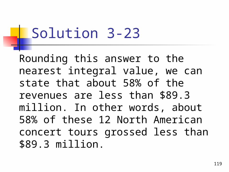
Solution 3-23
Rounding this answer to the nearest integral value, we can state that about 58% of the revenues are less than $89.3 million. In other words, about 58% of these 12 North American concert tours grossed less than $89.3 million.
120
BOX-AND-WHISKER PLOT
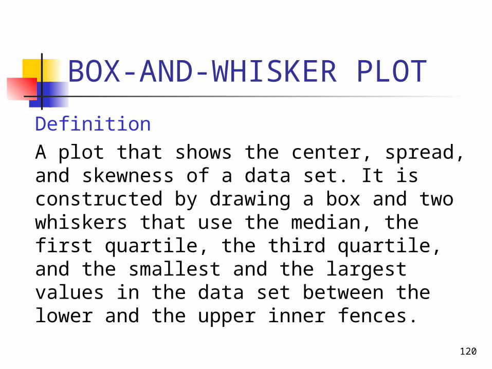
Definition A plot that shows the center, spread, and
skewness of a data set. It is constructed by drawing a box and two whiskers that use the median, the first quartile, the third quartile, and the smallest and the largest values in the data set between the lower and the upper inner fences.
121
Example 3-24
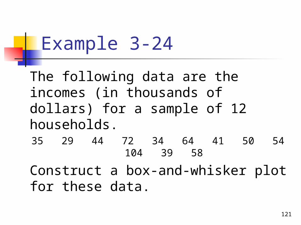
The following data are the incomes (in thousands of dollars) for a sample of 12 households.
35 29 44 72 34 64 41 50 54 104 39 58
Construct a box-and-whisker plot for these data.
122
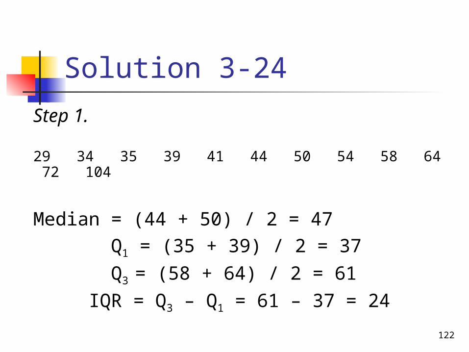
Solution 3-24 Step 1.
29 34 35 39 41 44 50 54 58 64 72 104
Median = (44 + 50) / 2 = 47 Q1 = (35 + 39) / 2 = 37 Q3 = (58 + 64) / 2 = 61 IQR = Q3 – Q1 = 61 – 37 = 24
123
Solution 3-24
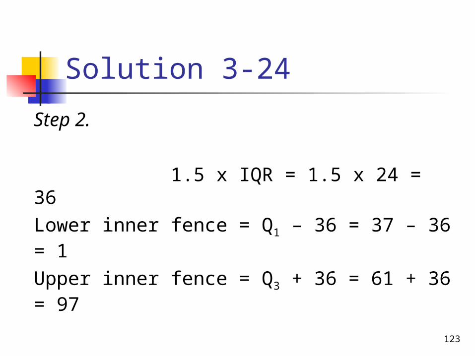
Step 2.
1.5 x IQR = 1.5 x 24 = 36 Lower inner fence = Q1 – 36 = 37 – 36
= 1 Upper inner fence = Q3 + 36 = 61 + 36
= 97

124
Solution 3-24
Step 3.
Smallest value within the two inner fences = 29
Largest value within the two inner fences = 72

125
Solution 3-24 Step 4. Figure 3.13
25 35 45 55 65 75 85 95 105Income
First quartile
Third quartile
Median

126
Solution 3-24 Step 5. Figure 3.14
25 35 45 55 65 75 85 95 105
An outlier
First quartile
Median
Third quartile
Smallest value within the two inner
fences
Largest value within two inner
fences
Income