Embed Size (px)
Citation preview

Chapter 3: Modelling
with Discrete Probability Distributions
In Chapter 2 we introduced several fundamental ideas: hypothesis testing, like-lihood, estimators, expectation, and variance. Each of these was illustrated bythe Binomial distribution. We now introduce several other discrete distribu-tions and discuss their properties and usage. First we revise Bernoulli trialsand the Binomial distribution.
Bernoulli Trials
A set of Bernoulli trials is a series of trials such that:
i) each trial has only 2 possible outcomes: Success and Failure;
ii) the probability of success, p, is constant for all trials;
iii) the trials are independent.
Examples: 1) Repeated tossing of a fair coin: each toss is a Bernoulli trial withP(success) = P(head) = 1
2 .
2) Having children: each child can be thought of as a Bernoulli trial withoutcomes {girl, boy} and P(girl) = 0.5.
3.1 Binomial distribution
Description: X ∼ Binomial(n, p) if X is the number of successes out of a fixednumber n of Bernoulli trials, each with P(success) = p.
Probability function: fX(x) = P(X = x) =(nx
)px(1− p)n−x for x = 0, 1, . . . , n.
Mean: E(X) = np.
Variance: Var(X) = np(1− p).
Sum of independent Binomials: IfX ∼ Binomial(n, p) and Y ∼ Binomial(m, p),and if X and Y are independent, and if X and Y both share the same parameterp, then X + Y ∼ Binomial(n+m, p).

93
Shape: Usually symmetrical unless p is close to 0 or 1.Peaks at approximately np.
0 1 2 3 4 5 6 7 8 9 10
0.0
0.05
0.10
0.15
0.20
0.25
0 1 2 3 4 5 6 7 8 9 10
0.0
0.1
0.2
0.3
0.4
0.0
0.02
0.04
0.06
0.08
0.10
0.12
80 90 100
n = 10, p = 0.5(symmetrical)
n = 10, p = 0.9(skewed for p close to 1)
n = 100, p = 0.9(less skew for p = 0.9 if n is large)
3.2 Geometric distribution
Like the Binomial distribution, the Geometric distribution is defined in termsof a sequence of Bernoulli trials.
• The Binomial distribution counts the number of successes out of a fixednumber of trials.
• The Geometric distribution counts the number of trials before the firstsuccess occurs.
This means that the Geometric distribution counts the number of failuresbefore the first success.
If every trial has probability p of success, we write: X ∼ Geometric(p).
Examples: 1) X =number of boys before the first girl in a family:X ∼ Geometric(p = 0.5).
2) Fish jumping up a waterfall. On every jump the fishhas probability p of reaching the top.Let X be the number of failed jumps beforethe fish succeeds.Then X ∼ Geometric(p).

94
Properties of the Geometric distribution
i) Description
X ∼ Geometric(p) if X is the number of failures before the first success in aseries of Bernoulli trials with P(success) = p.
ii) Probability function
For X ∼ Geometric(p),
fX(x) = P(X = x) = (1− p)xp for x = 0, 1, 2, . . .
Explanation: P(X = x) = (1− p)x︸ ︷︷ ︸need x failures
× p︸︷︷︸final trial must be a success
Difference between Geometric and Binomial: For the Geometric distribu-tion, the trials must always occur in the order FF . . . F︸ ︷︷ ︸
x failures
S.
For the Binomial distribution, failures and successes can occur in any order:e.g. FF . . . FS, FSF . . . F , SF . . . F , etc.
This is why the Geometric distribution has probability function
P(x failures, 1 success) = (1− p)xp,
while the Binomial distribution has probability function
P(x failures, 1 success) =
(x+ 1
x
)(1− p)xp.
iii) Mean and variance
For X ∼ Geometric(p),
E(X) =1− pp
=q
p
Var(X) =1− pp2
=q
p2
95
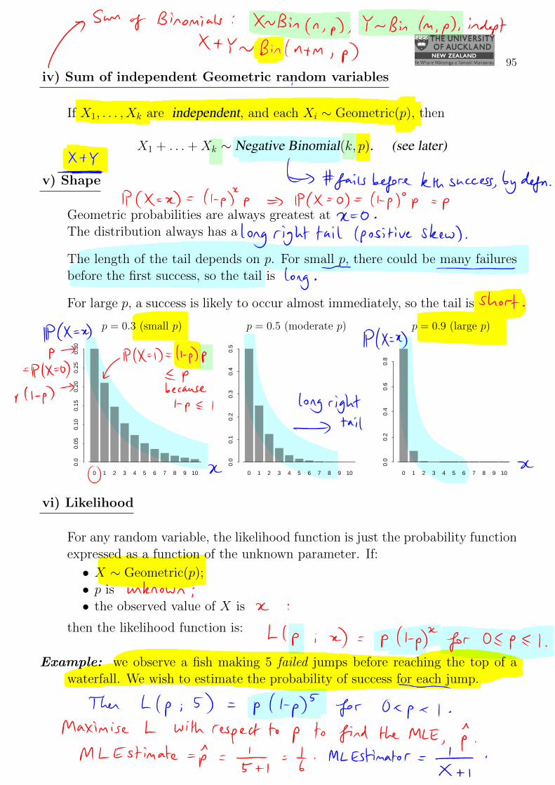
iv) Sum of independent Geometric random variables
If X1, . . . , Xk are independent, and each Xi ∼ Geometric(p), then
X1 + . . .+Xk ∼ Negative Binomial(k, p). (see later)
v) Shape
Geometric probabilities are always greatest at x = 0.The distribution always has a long right tail (positive skew).
The length of the tail depends on p. For small p, there could be many failuresbefore the first success, so the tail is long.
For large p, a success is likely to occur almost immediately, so the tail is short.
0 1 2 3 4 5 6 7 8 9 10
0.0
0.05
0.10
0.15
0.20
0.25
0.30
0 1 2 3 4 5 6 7 8 9 10
0.0
0.1
0.2
0.3
0.4
0.5
0 1 2 3 4 5 6 7 8 9 10
0.0
0.2
0.4
0.6
0.8
p = 0.3 (small p) p = 0.5 (moderate p) p = 0.9 (large p)
vi) Likelihood
For any random variable, the likelihood function is just the probability functionexpressed as a function of the unknown parameter. If:
• X ∼ Geometric(p);
• p is unknown;
• the observed value of X is x;
then the likelihood function is: L(p ;x) = p(1− p)x for 0 < p < 1.
Example: we observe a fish making 5 failed jumps before reaching the top of awaterfall. We wish to estimate the probability of success for each jump.
Then L(p ; 5) = p(1− p)5 for 0 < p < 1.
Maximize L with respect to p to find the MLE, p.

96
For mathematicians: proof of Geometric mean and variance formulae
(non-examinable)
We wish to prove that E(X) = 1−pp and Var(X) = 1−p
p2 when X ∼ Geometric(p).
We use the following results:
∞∑
x=1
xqx−1 =1
(1− q)2(for |q| < 1), (3.1)
and ∞∑
x=2
x(x− 1)qx−2 =2
(1− q)3(for |q| < 1). (3.2)
Proof of (3.1) and (3.2):
Consider the infinite sum of a geometric progression:
∞∑
x=0
qx =1
1− q (for |q| < 1).
Differentiate both sides with respect to q:
d
dq
( ∞∑
x=0
qx
)=
d
dq
(1
1− q
)
∞∑
x=0
d
dq(qx) =
1
(1− q)2
∞∑
x=1
xqx−1 =1
(1− q)2, as stated in (3.1).
Note that the lower limit of the summation becomes x = 1 because the termfor x = 0 vanishes.
The proof of (3.2) is obtained similarly, by differentiating both sides of (3.1)with respect to q (Exercise).

97
Now we can find E(X) and Var(X).
E(X) =∞∑
x=0
xP(X = x)
=∞∑
x=0
xpqx (where q = 1− p)
= p∞∑
x=1
xqx (lower limit becomes x = 1 because term in x = 0 is zero)
= pq∞∑
x=1
xqx−1
= pq
(1
(1− q)2
)(by equation (3.1))
= pq
(1
p2
)(because 1− q = p)
=q
p, as required.
For Var(X), we use
Var(X) = E(X2)− (EX)2 = E {X(X − 1)}+ E(X)− (EX)2 . (?)
Now
E{X(X − 1)} =∞∑
x=0
x(x− 1)P(X = x)
=∞∑
x=0
x(x− 1)pqx (where q = 1− p)
= pq2∞∑
x=2
x(x− 1)qx−2 (note that terms below x = 2 vanish)
= pq2
(2
(1− q)3
)(by equation (3.2))
=2q2
p2.
Thus by (?),Var(X) =
2q2
p2+q
p−(q
p
)2
=q(q + p)
p2=
q
p2,
as required, because q + p = 1.

98
3.3 Negative Binomial distribution
The Negative Binomial distribution is a generalised form of the Geometric dis-tribution:
• the Geometric distribution counts the number of failures before the firstsuccess;
• the Negative Binomial distribution counts the number of failures beforethe k’th success.
If every trial has probability p of success, we write: X ∼ NegBin(k, p).
Examples: 1) X =number of boys before the second girl in a family:X ∼ NegBin(k = 2, p = 0.5).
?2) Tom needs to pass 24 papers to complete his degree.He passes each paper with probability p, independentlyof all other papers. Let X be the number of papersTom fails in his degree.
Then X ∼ NegBin(24, p).
Properties of the Negative Binomial distribution
i) Description
X ∼ NegBin(k, p) if X is the number of failures before the k’th successin a series of Bernoulli trials with P(success) = p.
ii) Probability function
For X ∼ NegBin(k, p),
fX(x) = P(X = x) =
(k + x− 1
x
)pk(1− p)x for x = 0, 1, 2, . . .

99
Explanation:
• For X = x, we need x failures and k successes.
• The trials stop when we reach the k’th success, so the last trial must be asuccess.
• This leaves x failures and k − 1 successes to occur in any order:a total of k − 1 + x trials.
For example, if x = 3 failures and k = 2 successes, we could have:
FFFSS FFSFS FSFFS SFFFS
So:
P(X = x) =
(k + x− 1
x
)
︸ ︷︷ ︸(k − 1) successes and x failures
out of (k − 1 + x) trials.
×k successes︷︸︸︷
pk × (1− p)x︸ ︷︷ ︸x failures
iii) Mean and variance
For X ∼ NegBin(k, p),
E(X) =k(1− p)
p=kq
p
Var(X) =k(1− p)
p2=kq
p2
These results can be proved from the fact that the Negative Binomial distribu-tion is obtained as the sum of k independent Geometric random variables:
X = Y1 + . . .+ Yk, where each Yi ∼ Geometric(p), Yi indept,
⇒ E(X) = kE(Yi) =kq
p,
Var(X) = kVar(Yi) =kq
p2.
iv) Sum of independent Negative Binomial random variables
If X and Y are independent,and X ∼ NegBin(k, p), Y ∼ NegBin(m, p), with the same value of p, then
X + Y ∼ NegBin(k +m, p).
100
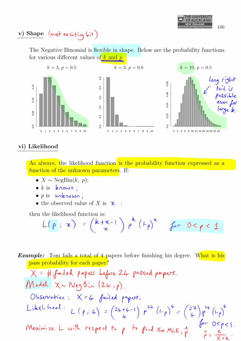
v) Shape
The Negative Binomial is flexible in shape. Below are the probability functionsfor various different values of k and p.
0 1 2 3 4 5 6 7 8 9 10
0.0
0.05
0.10
0.15
0 1 2 3 4 5 6 7 8 9 10
0.0
0.1
0.2
0.3
0.4
0.5
0 2 4 6 8 10 12 14 16 18 20 22 24
0.0
0.02
0.04
0.06
0.08
k = 3, p = 0.5 k = 3, p = 0.8 k = 10, p = 0.5
vi) Likelihood
As always, the likelihood function is the probability function expressed as afunction of the unknown parameters. If:
• X ∼ NegBin(k, p);
• k is known;
• p is unknown;
• the observed value of X is x;
then the likelihood function is:
L(p ;x) =
(k + x− 1
x
)pk(1− p)x for 0 < p < 1.
Example: Tom fails a total of 4 papers before finishing his degree. What is hispass probability for each paper?
X =# failed papers before 24 passed papers: X ∼ NegBin(24, p).
Observation: X = 4 failed papers.Likelihood:
L(p ; 4) =
(24 + 4− 1
4
)p24(1− p)4 =
(27
4
)p24(1− p)4 for 0 < p < 1.
Maximize L with respect to p to find the MLE, p.

101
3.4 Hypergeometric distribution: sampling without replacement
The hypergeometric distribution is used when we are sampling without replace-ment from a finite population.
i) Description
Suppose we have N objects:
• M of the N objects are special;• the other N −M objects are not special.
We remove n objects at random without replacement.
Let X = number of the n removed objects that are special.
Then X ∼ Hypergeometric(N, M, n).
Example: Ron has a box of Chocolate Frogs. There are 20 chocolate frogs in thebox. Eight of them are dark chocolate, and twelve of them are white chocolate.
Ron grabs a random handful of 5 chocolate frogs and stuffs them into his mouthwhen he thinks that noone is looking. Let X be the number of dark chocolatefrogs he picks.
Then X ∼ Hypergeometric(N = 20, M = 8, n = 5).
ii) Probability function
For X ∼ Hypergeometric(N,M, n),
fX(x) = P(X = x) =
(Mx
)(N−Mn−x
)(Nn
)
for x = max(0, n+M −N) to x = min(n,M).

102
Explanation: We need to choose x special objects and n− x other objects.
• Number of ways of selecting x special objects from the M available is:(Mx
).
• Number of ways of selecting n−x other objects from the N −M availableis:(N−Mn−x
).
• Total number of ways of choosing x special objects and (n−x) other objectsis:(Mx
)×(N−Mn−x
).
• Overall number of ways of choosing n objects from N is:(Nn
).
Thus:
P(X = x) =number of desired ways
total number of ways=
(Mx
)(N−Mn−x
)(Nn
) .
Note: We need 0 ≤ x ≤M (number of special objects),and 0 ≤ n− x ≤ N −M (number of other objects).After some working, this gives us the stated constraint that
x = max(0, n+M −N) to x = min(n,M).
Example: What is the probability that Ron selects 3 white and 2 dark chocolates?
X =# dark chocolates. There are N = 20 chocolates, including M = 8 darkchocolates. We need
P(X = 2) =
(82
)(123
)(
205
) =28× 220
15504= 0.397 .
iii) Mean and variance
For X ∼ Hypergeometric(N,M, n),
E(X) = np
Var(X) = np(1− p)(N−nN−1
) where p = MN .

103
iv) Shape
The Hypergeometric distribution is similar to the Binomial distribution whenn/N is small, because removing n objects does not change the overall compo-sition of the population very much when n/N is small.
For n/N < 0.1 we often approximate the Hypergeometric(N,M, n) distributionby the Binomial(n, p = M
N ) distribution.
0 1 2 3 4 5 6 7 8 9 10
0.0
0.05
0.10
0.15
0.20
0.25
0.30
0 1 2 3 4 5 6 7 8 9 10
0.0
0.05
0.10
0.15
0.20
0.25
Hypergeometric(30, 12, 10) Binomial(10, 1230)
Note: The Hypergeometric distribution can be used for opinion polls, becausethese involve sampling without replacement from a finite population.
The Binomial distribution is used when the population is sampled with replace-ment.
As noted above, Hypergeometric(N,M, n)→ Binomial(n, MN ) as N →∞.
A note about distribution names
Discrete distributions often get their names from mathematical power series.
• Binomial probabilities sum to 1 because of the Binomial Theorem:(p+ (1− p)
)n= <sum of Binomial probabilities> = 1.
• Negative Binomial probabilities sum to 1 by the Negative Binomial expan-sion: i.e. the Binomial expansion with a negative power, −k:
pk(
1− (1− p))−k
= <sum of NegBin probabilities> = 1.
• Geometric probabilities sum to 1 because they form a Geometric series:
p∞∑
x=0
(1− p)x = <sum of Geometric probabilities> = 1.

3.5 Poisson distribution
When is the next volcano due to erupt in Auckland?
Any moment now, unfortunately!(give or take 1000 years or so. . . )
A volcano could happen in Auckland this afternoon, or it might not happen foranother 1000 years. Volcanoes are almost impossible to predict: they seem tohappen completely at random.
A distribution that counts the number of random events in a fixed spaceof time is the Poisson distribution.
How many cars will cross the Harbour Bridge today? X ∼ Poisson.How many road accidents will there be in NZ this year? X ∼ Poisson.How many volcanoes will erupt over the next 1000 years? X ∼ Poisson.
The Poisson distribution arose from a mathematical
formulation called the Poisson Process, published
by Simeon-Denis Poisson in 1837.
Poisson Process
The Poisson process counts the number of events occurring in a fixedtime or space, when events occur independently and at a constantaverage rate.
Example: Let X be the number of road accidents in a year in New Zealand.Suppose that:
i) all accidents are independent of each other;
ii) accidents occur at a constant average rate of λ per year;
iii) accidents cannot occur simultaneously.
Then the number of accidents in a year, X, has the distribution
X ∼ Poisson(λ).
105
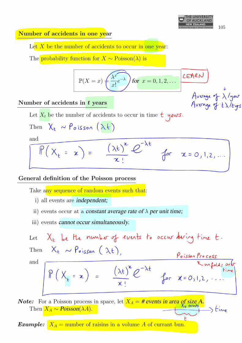
Number of accidents in one year
Let X be the number of accidents to occur in one year: X ∼ Poisson(λ).
The probability function for X ∼ Poisson(λ) is
P(X = x) =λx
x!e−λ for x = 0, 1, 2, . . .
Number of accidents in t years
Let Xt be the number of accidents to occur in time t years.
Then Xt ∼ Poisson(λt),
and
P(Xt = x) =(λt)x
x!e−λt for x = 0, 1, 2, . . .
General definition of the Poisson process
Take any sequence of random events such that:
i) all events are independent;
ii) events occur at a constant average rate of λ per unit time;
iii) events cannot occur simultaneously.
Let Xt be the number of events to occur in time t.
Then Xt ∼ Poisson(λt),
and
P(Xt = x) =(λt)x
x!e−λt for x = 0, 1, 2, . . .
Note: For a Poisson process in space, let XA = # events in area of size A.Then XA ∼ Poisson(λA).
Example: XA = number of raisins in a volume A of currant bun.

106
Where does the Poisson formula come from?
(Sketch idea, for mathematicians; non-examinable).The formal definition of the Poisson process is as follows.
Definition: The random variables {Xt : t > 0} form a Poisson process with rate λ if:
i) events occurring in any time interval are independent of those occurringin any other disjoint time interval;
ii)
limδt↓0
(P(exactly one event occurs in time interval[t, t+ δt])
δt
)= λ ;
iii)
limδt↓0
(P(more than one event occurs in time interval[t, t+ δt])
δt
)= 0 .
These conditions can be used to derive a partial differential equation on a func-tion known as the probability generating function of Xt. The partial differentialequation is solved to provide the form P(Xt = x) = (λt)x
x! e−λt.
Poisson distribution
The Poisson distribution is not just used in the context of the Poisson process.It is also used in many other situations, often as a subjective model (see Section3.7). Its properties are as follows.
i) Probability function
For X ∼ Poisson(λ),
fX(x) = P(X = x) =λx
x!e−λ for x = 0, 1, 2, . . .
The parameter λ is called the rate of the Poisson distribution.

107
ii) Mean and variance
The mean and variance of the Poisson(λ) distribution are both λ.
E(X) = Var(X) = λ when X ∼ Poisson(λ).
Notes:
1. It makes sense for E(X) = λ: by definition, λ is the average number of eventsper unit time in the Poisson process.
2. The variance of the Poisson distribution increases with the mean (in fact,variance = mean). This is often the case in real life: there is more uncertaintyassociated with larger numbers than with smaller numbers.
iii) Sum of independent Poisson random variables
If X and Y are independent, and X ∼ Poisson(λ), Y ∼ Poisson(µ), then
X + Y ∼ Poisson(λ+ µ).
iv) Shape
The shape of the Poisson distribution depends upon the value of λ. For smallλ, the distribution has positive (right) skew. As λ increases, the distributionbecomes more and more symmetrical, until for large λ it has the familiar bell-shaped appearance.
The probability functions for various λ are shown below.
0 1 2 3 4 5 6 7 8 9 10
0.0
0.1
0.2
0.3
0 1 2 3 4 5 6 7 8 9 10
0.0
0.05
0.10
0.15
0.20
0.0
0.01
0.02
0.03
0.04
60 80 100 120 140
λ = 1 λ = 3.5 λ = 100

108
v) Likelihood and Estimator Variance
As always, the likelihood function is the probability function expressed as afunction of the unknown parameters. If:
• X ∼ Poisson(λ);
• λ is unknown;
• the observed value of X is x;
then the likelihood function is:
L(λ; x) =λx
x!e−λ for 0 < λ <∞.
Example: 28 babies were born in Mt Roskill yesterday. Estimate λ.
Let X =# babies born in a day in Mt Roskill. Assume that X ∼Poisson(λ).
Observation: X = 28 babies.Likelihood:
L(λ ; 28) =λ28
28!e−λ for 0 < λ <∞.
Maximize L with respect to λ to find the MLE, λ.We find that λ = x = 28.Similarly, the maximum likelihood estimator of λ is: λ = X.
Thus the estimator variance is:
Var(λ) = Var(X) = λ, because X ∼ Poisson(λ).
Because we don’t know λ, we have to estimate the variance:
Var(λ) = λ.
vi) R command for the p-value:
If X ∼ Poisson(λ), then the R command for P(X ≤ x) is ppois(x, lambda).
Proof of Poisson mean and variance formulae (non-examinable)
We wish to prove that E(X) = Var(X) = λ for X ∼ Poisson(λ).
ForX ∼ Poisson(λ), the probability function is fX(x) =λx
x!e−λ for x = 0, 1, 2, . . .
109
So
E(X) =∞∑
x=0
xfX(x) =∞∑
x=0
x
(λx
x!e−λ)
=∞∑
x=1
λx
(x− 1)!e−λ (note that term for x = 0 is 0)
= λ∞∑
x=1
λx−1
(x− 1)!e−λ (writing everything in terms of x− 1)
= λ∞∑
y=0
λy
y!e−λ (putting y = x− 1)
= λ, because the sum=1 (sum of Poisson probabilities) .
So E(X) = λ, as required.
For Var(X), we use: Var(X) = E(X2)− (EX)2
= E[X(X − 1)] + E(X)− (EX)2
= E[X(X − 1)] + λ− λ2.
But E[X(X − 1)] =∞∑
x=0
x(x− 1)λx
x!e−λ
=∞∑
x=2
λx
(x− 2)!e−λ (terms for x = 0 and x = 1 are 0)
= λ2∞∑
x=2
λx−2
(x− 2)!e−λ (writing everything in terms of x− 2)
= λ2∞∑
y=0
λy
y!e−λ (putting y = x− 2)
= λ2.
SoVar(X) = E[X(X − 1)] + λ− λ2
= λ2 + λ− λ2
= λ, as required.

110
3.6 Likelihood and log-likelihood for n independent observations
So far, we have seen how to calculate the maximum likelihood estimator in thecase of a single observation made from a distribution:
• Y ∼ Binomial(n, p) where n is known and p is to be estimated.
Maximum likelihood estimator: p = Yn .
• Y ∼ Geometric(p). Maximum likelihood estimator: p = 1Y+1 .
• Y ∼ NegBin(k, p) where k is known and p is to be estimated.
Maximum likelihood estimator: p = kY+k .
• Y ∼ Poisson(λ). Maximum likelihood estimator: λ = Y .
Question: What would we do if we had n independent observations, Y1, Y2, . . . , Yn?
Answer: As usual, the likelihood function is defined as the probability of thedata, expressed as a function of the unknown parameter.
If the data consist of several independent observations, their probability isgained by multiplying the individual probabilities together.
Example: Suppose we have observations Y1, Y2, . . . , Yn where each Yi ∼ Poisson(λ),and Y1, . . . , Yn are independent. Find the maximum likelihood estimator of λ.
Before we start, what would you guess λ to be in this situation?
Solution: For observations Y1 = y1, . . . , Yn = yn, the likelihood is:
L(λ ; y1, . . . , yn) = P(Y1 = y1, Y2 = y2, . . . , Yn = yn) under parameter λ
= P(Y1 = y1 ∩ Y2 = y2 ∩ . . . ∩ Yn = yn)
= P(Y1 = y1)P(Y2 = y2) . . .P(Yn = yn) by independence
=n∏
i=1
(λyi
yi !e−λ)
=
(n∏
i=1
1
yi !
)(e−λ)nλ(y1+y2+...+yn)
= Ke−nλ λny .

111
So L(λ ; y1, . . . , yn) = Ke−nλ λny ,
where y = 1n
∑ni=1 yi, and K =
∏ni=1
1yi ! is a constant that doesn’t depend on λ.
Differentiate L(λ ; y1, . . . , yn) and set to 0 to find the MLE:
0 =d
dλL(λ ; y1, . . . , yn)
= K{−ne−nλ λny + (ny) e−nλ λ(ny−1)
}
= Ke−nλλ(ny−1) {−nλ+ (ny)}⇒ λ =∞, λ = 0, or λ = y.
If we know that L(λ ; y1, . . . , yn) reaches a unique maximum in 0 < λ <∞, forexample by reference to a graph, then we can deduce that the MLE is y.
So the maximum likelihood estimator is:
λ = Y =Y1 + . . .+ Yn
n.
Note: When n = 1, we get the same result as we had before: λ = Y11 = Y1.
Log-likelihood
Instead of maximizing the likelihood function L to find the MLE, we often takelogs and maximize the log-likelihood function, logL. (Note: log = loge = ln.)
There are several reasons for using the log-likelihood:1. The logarithmic function L 7→ log(L) is increasing, so the functions L(λ)
and log {L(λ)} will have the same maximum, λ.
2. When there are observations Y1, . . . , Yn, the likelihood L is a product. Be-cause log(ab) = log(a) + log(b), the log-likelihood converts the productinto a sum. It is often easier to differentiate a sum than a product, sothe log-likelihood is easier to maximize while still giving the same MLE.
3. If we need to use a computer to calculate and maximize the likelihood, therewill often be numerical problems with computing the likelihood product,whereas the log-likelihood sum can be accurately calculated.
112
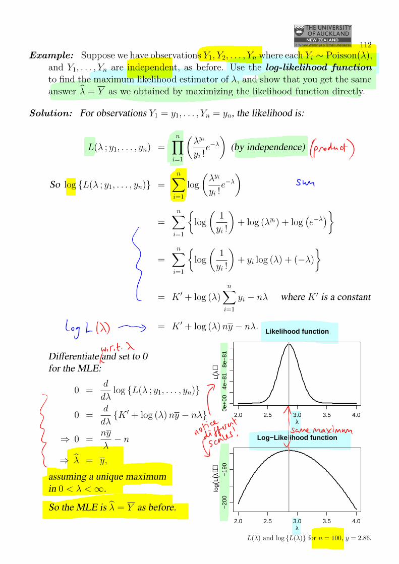
Example: Suppose we have observations Y1, Y2, . . . , Yn where each Yi ∼ Poisson(λ),and Y1, . . . , Yn are independent, as before. Use the log-likelihood functionto find the maximum likelihood estimator of λ, and show that you get the sameanswer λ = Y as we obtained by maximizing the likelihood function directly.
Solution: For observations Y1 = y1, . . . , Yn = yn, the likelihood is:
L(λ ; y1, . . . , yn) =n∏
i=1
(λyi
yi !e−λ)
(by independence)
So log {L(λ ; y1, . . . , yn)} =n∑
i=1
log
(λyi
yi !e−λ)
=n∑
i=1
{log
(1
yi !
)+ log (λyi) + log
(e−λ)}
=n∑
i=1
{log
(1
yi !
)+ yi log (λ) + (−λ)
}
= K ′ + log (λ)n∑
i=1
yi − nλ where K ′ is a constant
= K ′ + log (λ)ny − nλ.
2.0 2.5 3.0 3.5 4.0
0e+
004e
−81
8e−
81
Likelihood function
λ
L(λ)
2.0 2.5 3.0 3.5 4.0
−20
0−
190
Log−Likelihood function
λ
log(
L(λ)
)
L(λ) and log {L(λ)} for n = 100, y = 2.86.
Differentiate and set to 0for the MLE:
0 =d
dλlog {L(λ ; y1, . . . , yn)}
0 =d
dλ{K ′ + log (λ)ny − nλ}
⇒ 0 =ny
λ− n
⇒ λ = y,
assuming a unique maximumin 0 < λ <∞.
So the MLE is λ = Y as before.

113
3.7 Subjective modelling
Most of the distributions we have talked about in this chapter are exact modelsfor the situation described. For example, the Binomial distribution describesexactly the distribution of the number of successes in n Bernoulli trials.
However, there is often no exact model available. If so, we will use a subjectivemodel.
In a subjective model, we pick a probability distribution to describe a situationjust because it has properties that we think are appropriate to the situation, suchas the right sort of symmetry or skew, or the right sort of relationship betweenvariance and mean.
Example: Distribution of word lengths for English words.
Let Y = number of letters in an English word chosen at random from the dictio-nary.
If we plot the frequencies on a barplot, we see that the shape of the distributionis roughly Poisson.
English word lengths: Y − 1 ∼ Poisson(6.22)
number of letters
pro
ba
bili
ty
0 5 10 15 20
0.0
0.0
50
.10
0.1
5
Word lengths from 25109 English words
The Poisson probabilities (with λ estimated by maximum likelihood) are plottedas points overlaying the barplot.We need to use Y ∼ 1 + Poisson because Y cannot take the value 0.The fit of the Poisson distribution is quite good.
114
In this example we can not say that the Poisson distribution represents thenumber of events in a fixed time or space: instead, it is being used as a subjectivemodel for word length.
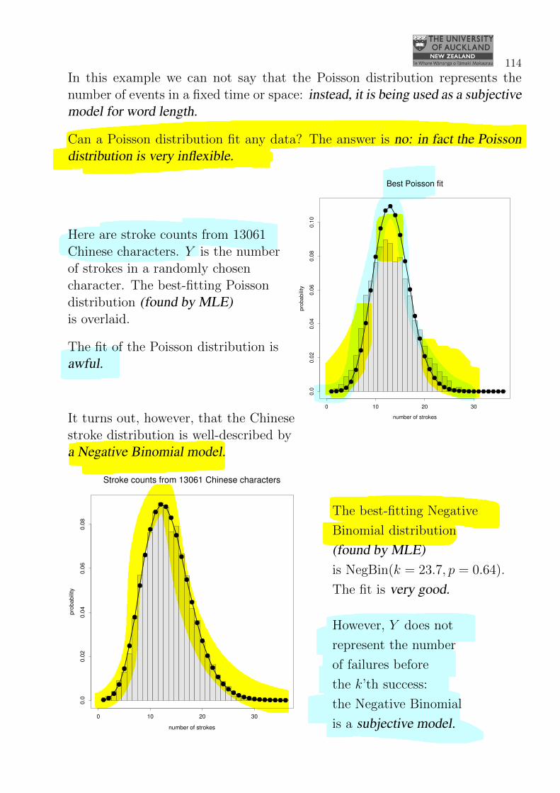
Can a Poisson distribution fit any data? The answer is no: in fact the Poissondistribution is very inflexible.
number of strokes
pro
ba
bili
ty
0 10 20 30
0.0
0.0
20
.04
0.0
60
.08
0.1
0
Best Poisson fit
Here are stroke counts from 13061Chinese characters. Y is the numberof strokes in a randomly chosencharacter. The best-fitting Poissondistribution (found by MLE)is overlaid.
The fit of the Poisson distribution isawful.
It turns out, however, that the Chinesestroke distribution is well-described bya Negative Binomial model.
number of strokes
pro
ba
bili
ty
0 10 20 30
0.0
0.0
20
.04
0.0
60
.08
Stroke counts from 13061 Chinese characters
The best-fitting Negative
Binomial distribution
(found by MLE)is NegBin(k = 23.7, p = 0.64).
The fit is very good.
However, Y does not
represent the number
of failures before
the k’th success:
the Negative Binomial
is a subjective model.

115
3.8 Statistical regression modelling
Statistical regression modelling is a fundamental technique used in data analysisin science and business. In this section we give an introduction to the idea ofregression modelling, using the simplest example of modelling a straight linethrough the origin of a scatterplot.
In statistical regression, we explore the relationship between two variables.
One variable, x, is typically under our control.
We select several different values of x. At each value of x, we make measure-ments of the other variable, Y .
The other variable, Y , is regarded as random.
The distribution of Y depends upon the value of x at which we measure it.
We write (xi, Yi) for the i’th pair of measurements, where i = 1, 2, . . . , n.
After the measurements are observed, we use lower-case letters and write (xi, yi).
Example: Where would you draw the best-fit line through the origin?
(x1, y1) = (1, 4)
(x2, y2) = (2, 5)
(x3, y3) = (3, 11)
●
05
1015
0 1 2 3 x
y
●
●
●
• x is called the predictor variable, because it predicts the distribution ofY .
• Y is called the response variable, because it is observed in response toselecting a particular value of x.
• You might sometimes see x called the ‘independent variable’ and Y called the‘dependent variable’. Although it is widely used, this terminology is confusingbecause x is not independent of Y in a statistical sense. Most statisticians avoidthis language and use the terms predictor and response instead.
116
How does the distribution of Y depend upon x?
In regression modelling, we generally assume that the MEAN of Y has somerelationship with the value of x.
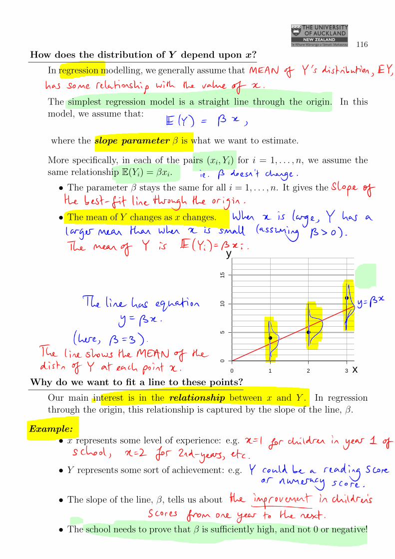
The simplest regression model is a straight line through the origin. In thismodel, we assume that:
E(Y ) = βx ,
where the slope parameter β is what we want to estimate.
More specifically, in each of the pairs (xi, Yi) for i = 1, . . . , n, we assume thesame relationship E(Yi) = βxi.
• The parameter β stays the same for all i = 1, . . . , n. It gives the slope ofthe best-fit line through the origin.
• The mean of Y changes as x changes. When x is large, Y has a largermean than when x is small (assuming β is positive). The meanof Y is E(Yi) = βxi.
The line has equation y = βx.
(Here, β = 3.)
The line shows the MEAN of thedistribution of Y at each point x.
●
05
1015
0 1 2 3 x
y
●
●
●
Why do we want to fit a line to these points?
Our main interest is in the relationship between x and Y . In regressionthrough the origin, this relationship is captured by the slope of the line, β.
Example:• x represents some level of experience: e.g. x = 1 for children in their
first year of school, x = 2 for 2nd-years, etc.
• Y represents some sort of achievement: e.g. Y could be a reading scoreor numeracy score.
• The slope of the line, β, tells us about the improvement in children’sscores from one year to the next.
• The school needs to prove that β is sufficiently high, and not 0 or negative!
117
Statistical model for Y
So far we have only specified the relationship between x and the mean of Y :E(Yi) = βxi.
In order to estimate the slope β, we need to specify the whole distributionof Y .
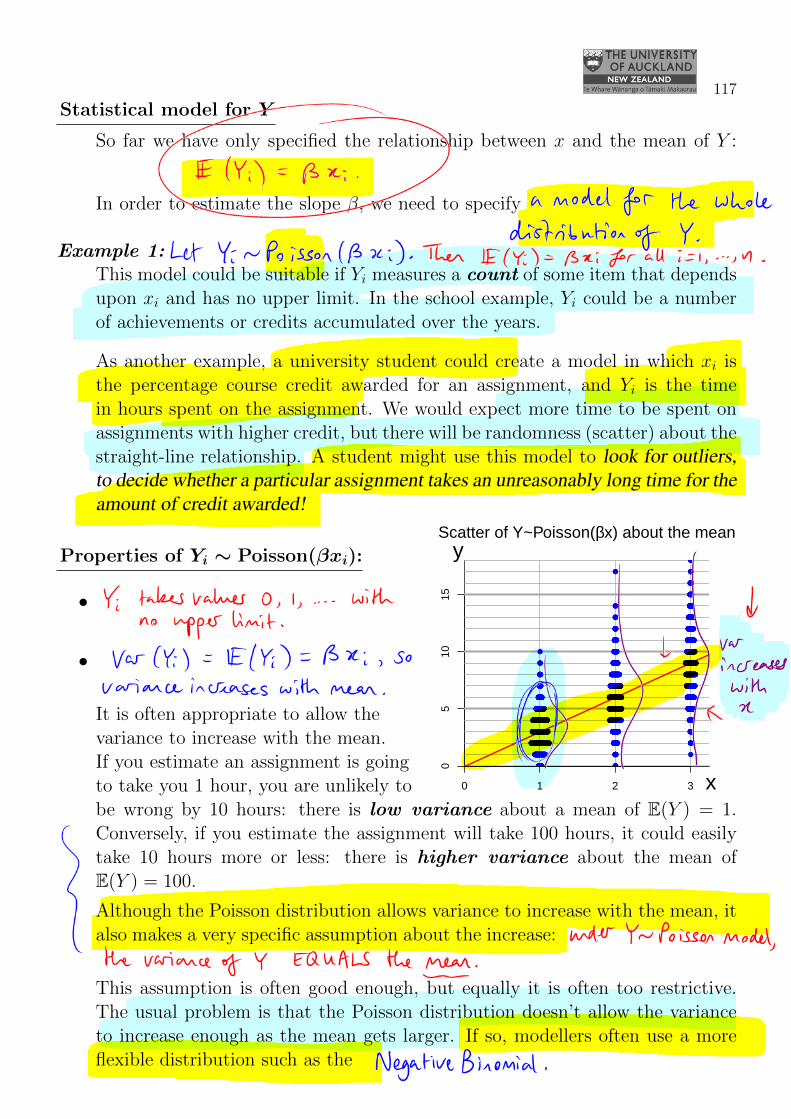
Example 1: Let Yi ∼ Poisson(βxi). Then E(Yi) = βxi for each i = 1, . . . , n.This model could be suitable if Yi measures a count of some item that dependsupon xi and has no upper limit. In the school example, Yi could be a numberof achievements or credits accumulated over the years.
As another example, a university student could create a model in which xi isthe percentage course credit awarded for an assignment, and Yi is the timein hours spent on the assignment. We would expect more time to be spent onassignments with higher credit, but there will be randomness (scatter) about thestraight-line relationship. A student might use this model to look for outliers,to decide whether a particular assignment takes an unreasonably long time for theamount of credit awarded!
●
05
1015
0 1 2 3 x
y
●●●●●●●●●●●●
●●●●●●●●●●●●●●●●●●●●●●●●●●●●●●●●●●●●●●●●●●●●●●●●●●●●●●●●●●●●●●●●●●●●●●●●●●●●●●●●●●●●●●●●●●●●●●●●●●●●●●●●●●●●●●●●●●●●●●●●●●●●●●●●●●●●●●●●●●●●●●●●●●●●●●●●●●●●●●●●●●●●●●●●●●●●●●●●●●●●●●●●●●●●●●●●●●●●●●●●●●●●
●●●●●●●●●●●●●●●●●●●●●●●●●●●●●●●●●●●●●●●●●●●●●●●●●●●●●●●●●●●●●●●●●●●●●●●●●●●●●●●●●●●●●●●●●●●●●●●●●●●●●●●●●●●●●●●●●●●●●●●●●●●●●●●●●●●●●●●●●●●●
●●●●●●●●●●●●●●●●●●●●●●●●●●●●●●●●●●●●●●●●●●●●●●●●●●●●●●●●●●●●●●●●●●●●●●●●●●●●●●●●●●●●●●●●●●●●●●●●●●●●●●●●●●●●●●●●●●●●●●●●●●●●●●●●●●●●●●●●●●●●●●●●●●●●●●●●●●●●●●●●●●●●●●●●●●●●●●●●●●●●●●●●●●●●●●●●●●●●●●●●●●●●●●●●●●●●●●●●●●●●●●●●●●●●●●●●●●●●
●●●●●●●●●●●●●●●●●●●●●●●●●●●●●●●●●●●●●●●●●●●●●●●●
●●●●●●●●●●●●●●●●●●●●●●●●●●●●●●●●●●●●●●●●●●●●●●●●●●●●●●●●●●●●●●●●●●●●●●●●●●●●●●●●●●●●●●●●●●●●●●●●●●●●●●●●●●●●●●●●●●●●●●●●●●●●●●●●●●●●●●●●●●●●●●●●●●●●●●●●●●●●●●●●●●●●●●●●●●●●●●●●●●●●●●●●●●●●●●●
●●●●●●●●●●●●●●●●●●●●●●●●●●●●●●●●●●●●●●●●●●
●●●●●●●●●●●●●●●●●●●●●●●●●●●●●●●●●●●●●●●●●●●●●●●●●●●●●●●●●●●●●●●●●●●●●●●●●●●●●●●●●●●●●●●●●●●●●●●●●●●●●●●●●
●●●●●●●●●●●●●●●●●●
●●●
●
●●●●●●●●●●●●●●●●●●●●●●●●●●●●●●●●●●●●●●●●●●●●●●●●●●●●●●●●●●●●●●●●●●●●●●●●●●●●●●●●●●●●●●●●●●●●●●●●●●●●●●●●●●●●●●●●●●●●●●●●●●●●●●●●●●●●●●●●●
●●●●●●●●●●●●●●●●●●●●●●●●●●●●●●●●●●●●●●●●●●●●●●●●●●●●●●●●●●●●●●●●●●●●●●●●●●●●●●●●●●●●●●●●●●●●●●●●●●●●●●●●●●●●●●●●●●●●●●●●●●●●●●●●●●●●●●●●●●●●●●●●●●●●●●●●●●●●●●●●
●●●●●●●●●●●●●●●●●●●●●●●●●●●●●●●●●●●●●●●●●●●●●●●●●●●●●●●●●●●●●●●●●●●●●●●●●●●●●●●●●●●●●●●●●●●●●●●●●●●●●●●●●●●●●●●●●●●●●●●●●●●●●●●●●●●●●●●●●●●●●●●●●●●●●●●●●●●●●●●●●
●●●●●
●●●●●●●●●●●●●●●●●●●●●●●●●●●●●●●●●●●●●●●●●●●●●●●●●●●●●●●●●●●●●●
●●●●●●●●●●●●●●●●●●●●●●●●●●●●●●●●●●●●●●●●●●●●●●●●●●●●●●●●●●●●●●●●●●●●●●●●●●●●●●●●●●●●●●●●●●●●●●●●●●●●●●●●●●●●●●●●●●●●●●●●●●●●●●●●●●●●●●●●●●●●●●●●●●●●●
●●●●●
●●●●●●●●●●●●●●●●●●●●●●●●●●●●●●●●●●●●
●●●●●●●●●●●●●●●●●●●●●●●●●●●●●●●●●●●●●●●●●●●●●●●●●
●●●●●●●●●●●●●●●●●●●●●●●●●●●●●●●●●●●●●●●●●●●●●●●●●●●●●●●●●●●●●●●●●●●●●●●●●●●●●●●●●●●●●●●●●●●●●●●●●●●●●●●●
●●●●●●●●●●●●●●●●●●●●●●●●●●●●●●●●●●●●●●●●●●●●●●●●●●●●●●●●●●●●●●●●●●●●●●●●●●●●
●●●●●●●●●●
●●●
●●●●●●●●●●●●●●●●●●●●●●●●●●●●●●
●●●●●●●●●●●
●●
●●●●●●●●●●●●●●●●●●●●●●●●●●●●●●●●
●●●●●●●●●●●●●●●●●●●●●●●●●●●●●●●●●●●●●●●●●●●●●●●●●●●●●●●●●●●●●●●●●●●●●●●●●●●●●●●●●●●●●●●●●●●
●●●●●●●●●●●●●●●●●●●●●●●●●●●●●●●●●●●●●●
●●●●●●●●●●●●●●●●●●●●●●●●●●●●●●●●●●●●●●●●●●●●●●●●●●●●●●●●●●●●●●●●●●●●●●●●●●●●●●●●●●●●●●●●●●●●●●●●●●●●●●●●
●●●●●●●●●●●●●●●●●●●●●●●●●●●●●●●●●●●●●●●●●●●●●●●●●●●●●●●●●●●●●●●●●●●●●●●●●●●●●●●●●●●●●●●●●●●●●●●●●●●●●●●●●●●●●
●●●●●●●●●●●●●●●●●●●●●●●●●●●●●●●●●●●●●●●●●●●●●●●●●●●●●●●●●●●●●●●●●●●●●●●●●●●●●●●●●●●●●●●
●●●●●●●●●●●●●●●●●●●●●●●●●●●●●●●●●●●●●●●●●●●●●●●●●●●●●●●●●●●●●●●●●●●●●●●●●●●●●●●●●●●●●●●●●●●●●●●●●●●●●●●●●●●●●●●●●●●●●●●●●●●●
●●●●●●●●●●●●●●●●●●●●●●●●●●●●●●●●●●●●●●●●●●●●●●●●●●●●●●●●●●●●●
●●●●●●●●●●●●●●●●●●●●●●●●●●●●●●●●●●●●●●●●●●●●●●●●●●●●●●●●●●●●●●●●●●●●●●●●●●●●●●●●●●●●●●●●●●●●●●●●●●●●●●●●●●●●●●●●●●●●●●●●●●●●●●●●●●●●●●●●
●●●●●●●●●●●●●●●●●●●●●●●●●●●●●●●●●●●●●●●●●●●●●●●●●●●●●●●●●●●●●●●●●●●●●●●●●●
●●●●●●●●●●●●●●●●●●●●●●●
●●●●●●●●●●●●●●●●●●●●●●●●●●●●●●●●●●●●●●●●●●●●●●●●●●●●●●●●●●●●●●●●●●●●●●
●●●●●●●●●●●●●●●●
●●●●●●●
●●●●●●●●●●●●●●●●●
●●●
●●●
●
●●●●
Scatter of Y~Poisson(βx) about the mean
Properties of Yi ∼ Poisson(βxi):
• Yi takes values 0, 1, 2, . . . withno upper limit.
• Var(Yi) = E(Yi) = βxi, so varianceincreases with the mean.
It is often appropriate to allow thevariance to increase with the mean.If you estimate an assignment is goingto take you 1 hour, you are unlikely tobe wrong by 10 hours: there is low variance about a mean of E(Y ) = 1.Conversely, if you estimate the assignment will take 100 hours, it could easilytake 10 hours more or less: there is higher variance about the mean ofE(Y ) = 100.
Although the Poisson distribution allows variance to increase with the mean, italso makes a very specific assumption about the increase: under the Poissondistribution, the variance is always EQUAL to the mean.
This assumption is often good enough, but equally it is often too restrictive.The usual problem is that the Poisson distribution doesn’t allow the varianceto increase enough as the mean gets larger. If so, modellers often use a moreflexible distribution such as the Negative Binomial.
118
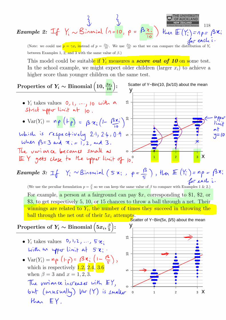
Example 2: If Yi ∼ Binomial(n = 10, p = βxi10 ), then E(Yi) = n× p = βxi for
each i.(Note: we could use p = γxi instead of p = βxi
10 . We use βxi
10 so that we can compare the distribution of Yi
between Examples 1, 2, and 3 with the same value of β.)
This model could be suitable if Yi measures a score out of 10 on some test.In the school example, we might expect older children (larger xi) to achieve ahigher score than younger children on the same test.
●
05
1015
0 1 2 3 x
y
●●●●●●●●●●●●●●●●●●●●●●●●●●●●●●●●●●●●●●●●●●●●●●●●●●●●●●●●●●●●●●●●●●●●●●●●●●●●●●●●●●●●●●●●●●●●●●●●●●●●●●●●●●●●●●●●●●●●●●●●●●●●●●●●●●●●●●●●●●●●●●●●●●●●●●●●●●●●●●●●●●●●●●●●●●●●●●●●●●●●●●●●●●●●●●●●●●●●●●●●●●●●●●●●●●●●●●●●●●●●●●●●●●●●●●●●●●●●●●●●●●●●●●●●●●●●●●●●●●●●●●●●●●●●●●●●
●●●●●●●●●●●●●●●●●●●●●●●●●●●●●●●●●●●●●●●●●●●●●●●●●●●●●●●●●●●●●●●●●●●●●●●●●●●●●●●●●●●●●●●●●●●●●●●●●●●●●●●●●●●●●●●●●●●●●●●●●●●●●●●●●●●●●●●●●●●●●●●●●●●●●●●●●●●●●●●●●●●●●●●●●●●●●●●●●●●●●●●●●●●●●●●●●●●●●●●●●●●●●●●●●●●●●●●●●●●●●●●●●●●●●●●●●●●●●●●●●●●●●●●
●●●●●●●●●●●●●●●●●●●●●●●●●●●●●●●●●●●●●●●●●●●●●●●●●●●●●●●●●●●●●●●●●●●●●●●●●●●●●●●●●●●●●●●●●●●●●●●●●●●●●●●●●●●●●●●●●●●●●●●●●●●●●●●●●●●●●●●●●●●●●●●●●●●●●●●●●●●●●●●●●●●●●●●●●●●●●●●●●●●●●●●●
●●●●●●●●●●●●●●●●●●●●●●●●●●●●●●●●●●●●●●●●●●●●●●●●●●●●●●●●●●●●●●●●●●●●●●●●●●●●●●●●●●●●●●●●●●●●●●●●●●●●●●●●●
●●●●●●●●●●●●●●●●●●●●●●●●●●●●●●●●●●●●●●●●●●●●●●●●●●●●●●●●●●●●●●●●●●●●●●●●●●●●●●●●●●●●●●●●●●●●●●●●●●●●●●●●●●●●●●●●●●●●●●●●
●●●●●●●●●●●●●●●●●●●●●●●●●●●●●●●●●●●
●●●●●●●●●●
●●●●●●●●●●●●●●●●●●●●●●●●●●●
●●●●●●●●●●●●●●●●●●●●●●●●●●●●●●●●●●●●●●●●●●●●●●●●●●●●●●●●●●●●●●●●●●●●●●●●●●●●●●●●●●●●●●●●●●●●●●●●●●●●●●●●●●●●●●●●●●●●●●●●●●●●●●●●●●●●●●●●●●●●●●●●●●●●●●●●●●●●●●●●●●●●●●●●●●●●●●●●●●●●●●●●●●●●●●●●●●●●●●●●●●●●●●●●●●●●●●●●●●●●●●●●●●●●●●●●●●●●●●●●●●
●●●●●●●●●●●●●●●●●●●●●●●●●●●●●●●●●●●●●●●●●●●●●●●●●●●●●●●●●●●●●●●●●●●●●●●●●●●●●●●●●●●●●●●●●●●●●●●●●●●●●●●●●●●●●●●●●●●●●●●●●●●●●●●●●●●●●●●●●●●●●●●●●●●●●●●●●●●●●●●●●●●●●●●●●●●●●●●●●●●●●●●●●●●●●●●●●●●●●●●●●●●●●●●●●●●●●●●●
●●●●●●●●●●●●●●●●●●●●●●●●●●●●●●●●●●●●●●●●●●●●●●●●●●●●●●●●●●●●●●●●●●●●●●●●●●●●●●●●●●●●●●●●●●●●●●●●●●●●●●●●●●●●●●●●●●●●●●
●●●●●●●●●●●●●●●●●●●●●●●●●●●●●●●●●●●●●●●●●●●●●●●●●●●●
●●●●●●●●●●●●●●●●●●●●●●●●●●●●●●●●●●●●●●●●●●●●●●●●●●●●●●●●●●●●●●●●●●●●●●●●●●●●●●●●●●●●●●●●●●●●●●●●●●●●●●●●●●●●●●●●●●●●●●●
●●●●●●●●●●●●●●●●●●●●●●●●●●●●●●●●●●●●●●●●●●●●●●●●●●●●●●●●●●●●●●●●●●●●●●●●●●●●●●●●●●●●●●●●●●●●●●●●●●●●●●●●●●●●●●●●●●●●●●●●●●●●●●●●●●●●●●●●●●●●●●●●●●●●●●●●●●●●●●●●●●●●●●●●●●●●●●●●●●●●●●●●●●●●●●●●
●●●●●●●●●●●●●●●●●●●●●●●●●●●●●●●●●●●●●●●●●●●●●●●●●●
●●●●●●
●●●●
●
●●●●●●●●●●●●●●●●●●●●●●●●●●●●●●●●●●●●●●●●●●●●●●●●●●●●●●●●●●●●●●●●●●●●●●●●●●●●●●●●●●●●●●●●●●●●●●●●●●●●●●●●●●●●●●●●●●●●●●●●●●●●●●●●●●●●●●●●●●●●●●●●●●●●●●●●●●●●●●●●●●●●●●
●●●●●●●●●●●●●●●●●●●●●●●●●●●●●●●●●●●●●●●●●●●●●●●●●●●●●●●●●●●●●●●●●●●●●●●●●●●●●●●●●●●●●●●●●●●●●●●●●●●●●●●●●●●●●●●●●●●●●●●●●●●●●●●●●●●●●●●●●●●●●●●●●●●●●●●●●●●●●●●●●●●●●●●●●●●●●●●●●●●●●●●●●●●●●●●●●●●●●●●●●●●●●●●●●●●●●●●●●●●●●●●●●●●●●●●●●●●●●●●●●●●●●●●●●●●●●●●●●●●●●●●●●●●●●●●●●●●●●●●●●●●●●●●●●●●●●●●●●●●●●●●●●●●●●●●●●●●●●●●●●●●●●●●●●●●●●●●●●●●●●●●●●●●●●●●●●●●●●●●●●●●●●●●●●●●●●●●●●●●●●●●●●●●●●●●●●●●
●●●●●●●●●●●●●●●●●●●●●●●●●●●●●●●●●●●●●●●●●●●●●●●●●●●●●●●●●●●●●●●●●●●●●●●●●●●●●●●●●●●●●●●●●●●●●●●●●●●●●●●●●●●●●●●●●●●●●●●●●●●●●●●●●●●●●●●●●●●●●●●●●●●●●●●●●●●●●●●●●●●●●●●●●●●●●●●●●●●●●●●●●●●●●●●●●●●●●●●●●●●●●●●●●●●●●●●●●●●●●●●●●●●●●●●●●●●●●●●●●●●●●●●●●●●●●●●●●●●●●●●●●●●●●●●●●●●●●●●●●●●●●●●●●●●●●●●●●●●●●●●●●●●●●●●●●●●●●●●●●●●●●●●●●●●●●●●●●●●●●●●●●●●●●●●●●●●●●●●●●●●●●●●●●
●●●●●●●●●●●●●●●
●●●●●●●●●●●●●●●●●●●●●●●●●●●●●●●●●●●●●●●●●●●●●●●●●●●●●
●●
Scatter of Y~Bin(10, βx/10) about the meanProperties of Yi ∼ Binomial(10, βxi
10
):
• Yi takes values 0, 1, 2, . . . , 10 witha strict upper limit at 10.
• Var(Yi) = np(1− p) = βxi
(1− βxi
10
),
which is respectively 2.1, 2.4, 0.9when β = 3 and x = 1, 2, 3.The variance becomes small as E(Y )gets close to the upper limit of 10.
Example 3: If Yi ∼ Binomial(n = 5xi, p = β5 ), then E(Yi) = n × p = βxi for
each i.(We use the peculiar formulation p = β
5 so we can keep the same value of β to compare with Examples 1 & 2.)
For example, a person at a fairground can pay $x, corresponding to $1, $2, or$3, to get respectively 5, 10, or 15 chances to throw a ball through a net. Theirwinnings are related to Yi, the number of times they succeed in throwing theball through the net out of their 5xi attempts.
●
05
1015
0 1 2 3 x
y
●●●●●●●●●●●●●●●●●●●●●●●●●●●●●●●●●●●●●●●●●●●●●●●●●●●●●●●●●●●●●●●●●●●●●●●●●●●●●●●●●●●●●●●●●●●●●●●●
●●●●●●●●●●●●●●●●●●●●●●●●●●●●●●●●●●●●●●●●●●●●●●●●●●●●●●●●●●●●●●●●●●●●●●●●●●●●●●●●●●●●●●●●●●●●●●●●●●●●●●●●●●●●●●●●●●●●●●●●●●●●●●●●●●●●●●●●●●●●●●●●●●●●●●●●●●●●●●●●●●●●●●●●●●●●●●●●●●●●●●●●●●●●●●●●●●●●●●●●●●●●●●●●●●●●●●●●●●●●
●●●●●●●●●●●●●●●●●●●●●●●●●●●●●●●●●●●●●●●●●●●●●●●●●●●●●●●●●●●●●●●●●●●●●●●●●●●●●●●●●●●●●●●●●●●●●●●●●●●●●●●●●●●●●●●●●●●●●●●●●●●●●●●●●●●●●●●●●●●●●●●●●●●●●●●●●●●●●●●●●●●●●●●●●●●●●●●●●●●●●●●●●●●●●●●●●●●●●●●●●●●●●●●●●●●●●●●●●●●●●●●●●●●●●●●●●●●●●●●●●●●●●●●●●●●●●●●●●●●●●●●●●●●●●●●●●●●●●●●●●●●●●●●●●●●●●●●●●●●●●●●●●●●●●●●●●●●●●●●●●●●●●●●●●●●●●●●
●●●●●●●●●●●●●●●●●●●●●●●●●●●●●●●●●●●●●●●●●●●●●●●●●●●●●●●●●●●●●●●●●●●●●●●●●●●●●●●●●●●
●●●●●●●●●●●●●●●●●●●●●●●●●●●●●●●●●●●●●●●●●●●●●●●●●●●●●●●●●●●●●●●●●●●●●●●●●●●●●●●●●●●●●●●●●●●●●●●●●●●●●●●●●●●●●●●●●●●●●●●●●●●●●●●●●●●●●●●●●●●●●●●●●●●●●●●●●●●●●●●●●●●●●●●●●●●●●●●●●●●●●●●●●●●●●●●●●●●●●●●●●●●●●●●●●●●●●●●●●●●●●●●●●●●●●●●●●●●●●●●●●●●●●●●●●●●●●●●●●●●●
●●●●●●
●●●●●●●●●●●●●●●●●●●●●●●●●●●●●●●●●●●●●●●●●●●●●●●●●●●●●●●●●●●●●●●●●●●●●●●●●●●●●●●●●●●●●●●●●●●●●●●●●●●●●●●●●●●●●●●●●●●●●●●●●●●●●●●●●●●●●●●●●●●●●●●●●●●●●●●●●●●●●●●●●●●●●●●●●●●●●●●●●●●●●●●●●●●●●●●●●●●●●●●●●●●●●●●●●●●●●●●●●●●●●●●●●●●●●●●●●●●●●●●●●●●●●●●●●●●●●●●●●●●●
●●●●●●●●●●●●●●●●●●●●●●●●●●●●●●●●●●●●●●●●●●●●●●●●●●●●●●●●●●●●●●●●●●●●●●●●●●●●●●●●●●●●●●●●●●●●●●●●●●●●●●●●●●●●●●●●●●●●●●●●●●●●●●●●●●●●●●●●●●●●●●●●●●●●●●●●●●●●●●●●●●●●●●●●●●●●●●●●●●●●●●●●●●●●●●●●●●●●●●●●●●●●●●●●●●●●●●●●●
●●●●●●●●●●●●●●●●●●●●●●●●●●●●●●●●●●●●●●●●●●●●●●●●●●●●●●●●●●●●●●●●●●●●●●●●●●●●●●●●●●●●●●●●●●●●●●●●●●●●●●●●●●
●●●●●●●●●●●●●●●●●●●●●●●●●●●●●●●●●●●●●●●●●●●●●●●●●●●●●●●●●●●●●●●●●●●●●●●●●●●●●●●●●●●●●●●●●●●●●●●●●●●●●●●●●●●●●●●●●●●●●●●●●●●●●●●●●●●●●●●●●●●●●●●●●●●●●●●●●●●●●●●●●●●●●●●●●●●●●●●●●●●●●●●●●●●●●●●●●●●●●●●●●●●
●●●●●●●●●●●●●●●●●●●●●●●●●●●●●●●●●●●●●●●●●●●●●●●●●●●●●●●●●●●●●●●●●●●●●●●●●●●●●●●●●●●●●●●●●●●●●●●●●●●●●●●●●●●●●●●●●●●●
●●●●●●●●●●●●●●●●●●●●●●●●●●●●●●●●●●●●●●●●●●●●●●
●●●●●●●●●●●●●●●●●●●●●●●●●●●●●●●●●●●●●
●●●●●●●●●●
●●●●
●
●●●●●●●●●●●●●●●●●●●●●●●●●●●●●●●●●●●●●●●●●●●●●●●●●●●●●●●●●●●●●●●●●●●●●●●●●●●●●●●●●●●●●●●●●●●●●●●●●●●●●●●●●●●●●●●●●●●●●●●●
●●●●●●●●●●●●●●●●●●●●●●●●●●●●●●●●●●●●●●●●●●●●●●●●●●●●●●●●●●●●●●●●●●●●●●●●●●●●●●●●●●●●●●●●●●●●●●●●●●●●●●●●●●●●●●●●●●●●●●●●●●●●●●●●●●●●●●●●●●●●●●●●●●●●●●●●●●●●●●●●●●●●●●●●●●●●●●●●●●●●●●●●●●●●●●●●●●
●●●●●●●●●●●●●●●●●●●●●●●●●●●●●●●●●●●●●●●●●●●●●●●●●●●●●●●●●●●●●●●●●●●●●●●●●●●●●●●●●●●●●●●●●●●●●●●●●●●●●●●●●●●●●●●●●●●●●●●●●●●●●●●●●●●●●●●●●●●●●●●●●●●●●●●●●●●●●●●●●●●●●●●●●●●●●●●●●●●●●●●●●●●●
●●●●●●●●●●●●●●●●●●●●●●●●●●●●●●●●●●●●●●●●●●●●●●●●●●●●●●●●●●●●●●●●●●●●
●●●●●●●●●●●●●●●●●
●●●●●●●●●●●●●●●●●●●●●●●●●●●●●●●●●●●●●●●●●●●●●●●●●●●●●●●●●●●●●●●●●●●●●●●●●●●●●●●●●●●●●●●●●●●●●●●●●●●●●●●●●●●●●●●●●●●●●●●●●●●●●●●●●●●●●●●●●●●●●●●●●●●●●●●●●●●●●●●●●●●●●●●●●●●
●●●●●●●●●●●●●●●●●●●●●●●●●●●●●●●●●●●●●●●●●●●●●●●●●●●●●●●●●●●●●●●●●●●●●●●●●●●
●●●●●●●●●●●●●●●●●●●●●●●●●●●●●●●●●●●●●●●●●●●●●●●●●●●●●●●●●●●●●●●●●●●●●●●●●●●●●●●●●●●●●●●●●●●●●●●●●●●●●●●●●●●●●●●●●●●●●●●●●●●●●●●●●●●●●●●●
●●●●●●●●●●●●●●●●
●●●●●●●●
●●●●●●
●
Scatter of Y~Bin(5x, β/5) about the mean
Properties of Yi ∼ Binomial(5xi,
β5
):
• Yi takes values 0, 1, 2, . . . , 5xi withan upper limit at 5xi.
• Var(Yi) = np(1− p) = βxi
(1− β
5
),
which is respectively 1.2, 2.4, 3.6when β = 3 and x = 1, 2, 3.The variance increases with E(Y )but (unusually) Var(Y ) is smallerthan E(Y ).
119
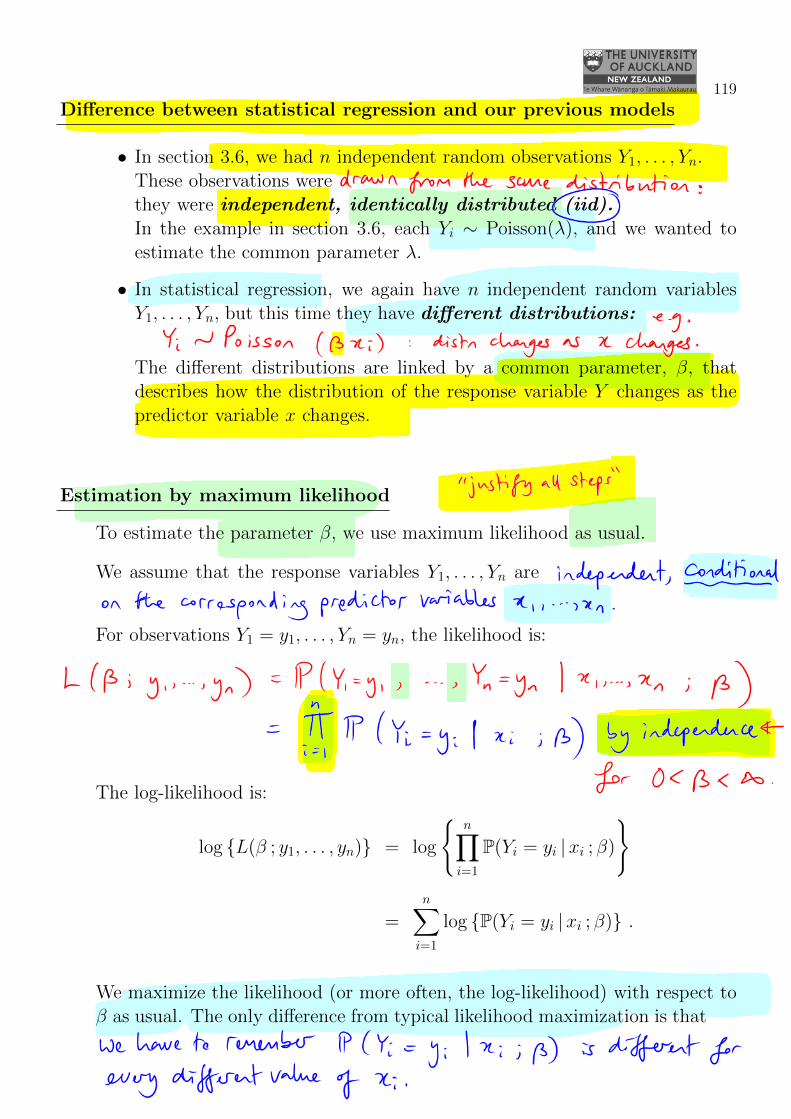
Difference between statistical regression and our previous models
• In section 3.6, we had n independent random observations Y1, . . . , Yn.These observations were drawn from the same distribution:they were independent, identically distributed (iid).In the example in section 3.6, each Yi ∼ Poisson(λ), and we wanted toestimate the common parameter λ.
• In statistical regression, we again have n independent random variablesY1, . . . , Yn, but this time they have different distributions: for exam-ple, Yi ∼ Poisson(βxi).
The different distributions are linked by a common parameter, β, thatdescribes how the distribution of the response variable Y changes as thepredictor variable x changes. Our interest is in estimating this pa-rameter β.
Estimation by maximum likelihood
To estimate the parameter β, we use maximum likelihood as usual.
We assume that the response variables Y1, . . . , Yn are independent, condi-tional on the corresponding predictor variables x1, . . . , xn.
For observations Y1 = y1, . . . , Yn = yn, the likelihood is:
L(β ; y1, . . . , yn) = P(Y1 = y1, Y2 = y2, . . . , Yn = yn |x1, . . . , xn ; β)
=n∏
i=1
P(Yi = yi |xi ; β) by independence.
The log-likelihood is:
log {L(β ; y1, . . . , yn)} = log
{n∏
i=1
P(Yi = yi |xi ; β)
}
=n∑
i=1
log {P(Yi = yi |xi ; β)} .
We maximize the likelihood (or more often, the log-likelihood) with respect toβ as usual. The only difference from typical likelihood maximization is that wehave to remember that P(Yi = yi |xi ; β) is different for every differentvalue of xi.

120
Example: Poisson regression
Recall the scenario shown at the beginning of this section:
(x1, y1) = (1, 4)
(x2, y2) = (2, 5)
(x3, y3) = (3, 11)
●
05
1015
0 1 2 3 x
y
●
●
●
Consider the model Yi ∼ Poisson(βxi), for i = 1, . . . , n.Maximize the likelihood to find the maximum likelihood estimator, β.
Also find the exact variance, Var(β) in terms of the unknown parameter β, and
suggest a suitable estimator Var(β) for the variance.
Evaluate β and Var(β) for the data shown above, where n = 3 and xi = i fori = 1, 2, 3. Mark your estimated best-fit line on the graph shown.
Solution: For Yi ∼ Poisson(βxi), the likelihood is (from the previous page):
L(β ; y1, . . . , yn) =n∏
i=1
P(Yi = yi |xi ; β)
=n∏
i=1
(βxi)yi
yi !e−βxi
=
(n∏
i=1
x yiiyi !
)β(y1+...+yn) e−β(x1+...+xn)
= K β(y1+...+yn) e−β(x1+...+xn)
where K is a constant: does not depend upon β
= K βny e−nxβ.

121
Differentiate and set to 0 for the MLE:
0 =d
dβL(β ; y1, . . . , yn)
=d
dβ
{K βny e−nxβ
}
= K{nyβ(ny−1) e−nxβ − βny nx e−nxβ
}
= Kβ(ny−1) e−nxβ {ny − βnx}
⇒ 0 = ny − βnx or β = 0,∞
⇒ β =y
x, assuming a unique maximum in 0 < β <∞.
So the MLE is:
β =Y
x=
Y1 + . . .+ Ynx1 + . . .+ xn
.
For the particular case (x1, y1) = (1, 4) ; (x2, y2) = (2, 5) ; (x3, y3) =(3, 11) , we have:
β =y1 + y2 + y3
x1 + x2 + x3
=4 + 5 + 11
1 + 2 + 3
=20
6
⇒ β = 3.33.
Add the best-fit line y = 3.33x to the graph overleaf by picking twopoints the line must go through: e.g. (x, y) = (0, 0) and (x, y) = (3, 10).
122
●
05
1015
0 1 2 3 x
y
●●●●●●●●●●●●
●●●●●●●●●●●●●●●●●●●●●●●●●●●●●●●●●●●●●●●●●●●●●●●●●●●●●●●●●●●●●●●●●●●●●●●●●●●●●●●●●●●●●●●●●●●●●●●●●●●●●●●●●●●●●●●●●●●●●●●●●●●●●●●●●●●●●●●●●●●●●●●●●●●●●●●●●●●●●●●●●●●●●●●●●●●●●●●●●●●●●●●●●●●●●●●●●●●●●●●●●●●●
●●●●●●●●●●●●●●●●●●●●●●●●●●●●●●●●●●●●●●●●●●●●●●●●●●●●●●●●●●●●●●●●●●●●●●●●●●●●●●●●●●●●●●●●●●●●●●●●●●●●●●●●●●●●●●●●●●●●●●●●●●●●●●●●●●●●●●●●●●●●
●●●●●●●●●●●●●●●●●●●●●●●●●●●●●●●●●●●●●●●●●●●●●●●●●●●●●●●●●●●●●●●●●●●●●●●●●●●●●●●●●●●●●●●●●●●●●●●●●●●●●●●●●●●●●●●●●●●●●●●●●●●●●●●●●●●●●●●●●●●●●●●●●●●●●●●●●●●●●●●●●●●●●●●●●●●●●●●●●●●●●●●●●●●●●●●●●●●●●●●●●●●●●●●●●●●●●●●●●●●●●●●●●●●●●●●●●●●●
●●●●●●●●●●●●●●●●●●●●●●●●●●●●●●●●●●●●●●●●●●●●●●●●
●●●●●●●●●●●●●●●●●●●●●●●●●●●●●●●●●●●●●●●●●●●●●●●●●●●●●●●●●●●●●●●●●●●●●●●●●●●●●●●●●●●●●●●●●●●●●●●●●●●●●●●●●●●●●●●●●●●●●●●●●●●●●●●●●●●●●●●●●●●●●●●●●●●●●●●●●●●●●●●●●●●●●●●●●●●●●●●●●●●●●●●●●●●●●●●
●●●●●●●●●●●●●●●●●●●●●●●●●●●●●●●●●●●●●●●●●●
●●●●●●●●●●●●●●●●●●●●●●●●●●●●●●●●●●●●●●●●●●●●●●●●●●●●●●●●●●●●●●●●●●●●●●●●●●●●●●●●●●●●●●●●●●●●●●●●●●●●●●●●●
●●●●●●●●●●●●●●●●●●
●●●
●
●●●●●●●●●●●●●●●●●●●●●●●●●●●●●●●●●●●●●●●●●●●●●●●●●●●●●●●●●●●●●●●●●●●●●●●●●●●●●●●●●●●●●●●●●●●●●●●●●●●●●●●●●●●●●●●●●●●●●●●●●●●●●●●●●●●●●●●●●
●●●●●●●●●●●●●●●●●●●●●●●●●●●●●●●●●●●●●●●●●●●●●●●●●●●●●●●●●●●●●●●●●●●●●●●●●●●●●●●●●●●●●●●●●●●●●●●●●●●●●●●●●●●●●●●●●●●●●●●●●●●●●●●●●●●●●●●●●●●●●●●●●●●●●●●●●●●●●●●●
●●●●●●●●●●●●●●●●●●●●●●●●●●●●●●●●●●●●●●●●●●●●●●●●●●●●●●●●●●●●●●●●●●●●●●●●●●●●●●●●●●●●●●●●●●●●●●●●●●●●●●●●●●●●●●●●●●●●●●●●●●●●●●●●●●●●●●●●●●●●●●●●●●●●●●●●●●●●●●●●●
●●●●●
●●●●●●●●●●●●●●●●●●●●●●●●●●●●●●●●●●●●●●●●●●●●●●●●●●●●●●●●●●●●●●
●●●●●●●●●●●●●●●●●●●●●●●●●●●●●●●●●●●●●●●●●●●●●●●●●●●●●●●●●●●●●●●●●●●●●●●●●●●●●●●●●●●●●●●●●●●●●●●●●●●●●●●●●●●●●●●●●●●●●●●●●●●●●●●●●●●●●●●●●●●●●●●●●●●●●
●●●●●
●●●●●●●●●●●●●●●●●●●●●●●●●●●●●●●●●●●●
●●●●●●●●●●●●●●●●●●●●●●●●●●●●●●●●●●●●●●●●●●●●●●●●●
●●●●●●●●●●●●●●●●●●●●●●●●●●●●●●●●●●●●●●●●●●●●●●●●●●●●●●●●●●●●●●●●●●●●●●●●●●●●●●●●●●●●●●●●●●●●●●●●●●●●●●●●
●●●●●●●●●●●●●●●●●●●●●●●●●●●●●●●●●●●●●●●●●●●●●●●●●●●●●●●●●●●●●●●●●●●●●●●●●●●●
●●●●●●●●●●
●●●
●●●●●●●●●●●●●●●●●●●●●●●●●●●●●●
●●●●●●●●●●●
●●
●●●●●●●●●●●●●●●●●●●●●●●●●●●●●●●●
●●●●●●●●●●●●●●●●●●●●●●●●●●●●●●●●●●●●●●●●●●●●●●●●●●●●●●●●●●●●●●●●●●●●●●●●●●●●●●●●●●●●●●●●●●●
●●●●●●●●●●●●●●●●●●●●●●●●●●●●●●●●●●●●●●
●●●●●●●●●●●●●●●●●●●●●●●●●●●●●●●●●●●●●●●●●●●●●●●●●●●●●●●●●●●●●●●●●●●●●●●●●●●●●●●●●●●●●●●●●●●●●●●●●●●●●●●●
●●●●●●●●●●●●●●●●●●●●●●●●●●●●●●●●●●●●●●●●●●●●●●●●●●●●●●●●●●●●●●●●●●●●●●●●●●●●●●●●●●●●●●●●●●●●●●●●●●●●●●●●●●●●●
●●●●●●●●●●●●●●●●●●●●●●●●●●●●●●●●●●●●●●●●●●●●●●●●●●●●●●●●●●●●●●●●●●●●●●●●●●●●●●●●●●●●●●●
●●●●●●●●●●●●●●●●●●●●●●●●●●●●●●●●●●●●●●●●●●●●●●●●●●●●●●●●●●●●●●●●●●●●●●●●●●●●●●●●●●●●●●●●●●●●●●●●●●●●●●●●●●●●●●●●●●●●●●●●●●●●
●●●●●●●●●●●●●●●●●●●●●●●●●●●●●●●●●●●●●●●●●●●●●●●●●●●●●●●●●●●●●
●●●●●●●●●●●●●●●●●●●●●●●●●●●●●●●●●●●●●●●●●●●●●●●●●●●●●●●●●●●●●●●●●●●●●●●●●●●●●●●●●●●●●●●●●●●●●●●●●●●●●●●●●●●●●●●●●●●●●●●●●●●●●●●●●●●●●●●●
●●●●●●●●●●●●●●●●●●●●●●●●●●●●●●●●●●●●●●●●●●●●●●●●●●●●●●●●●●●●●●●●●●●●●●●●●●
●●●●●●●●●●●●●●●●●●●●●●●
●●●●●●●●●●●●●●●●●●●●●●●●●●●●●●●●●●●●●●●●●●●●●●●●●●●●●●●●●●●●●●●●●●●●●●
●●●●●●●●●●●●●●●●
●●●●●●●
●●●●●●●●●●●●●●●●●
●●●
●●●
●
●●●●
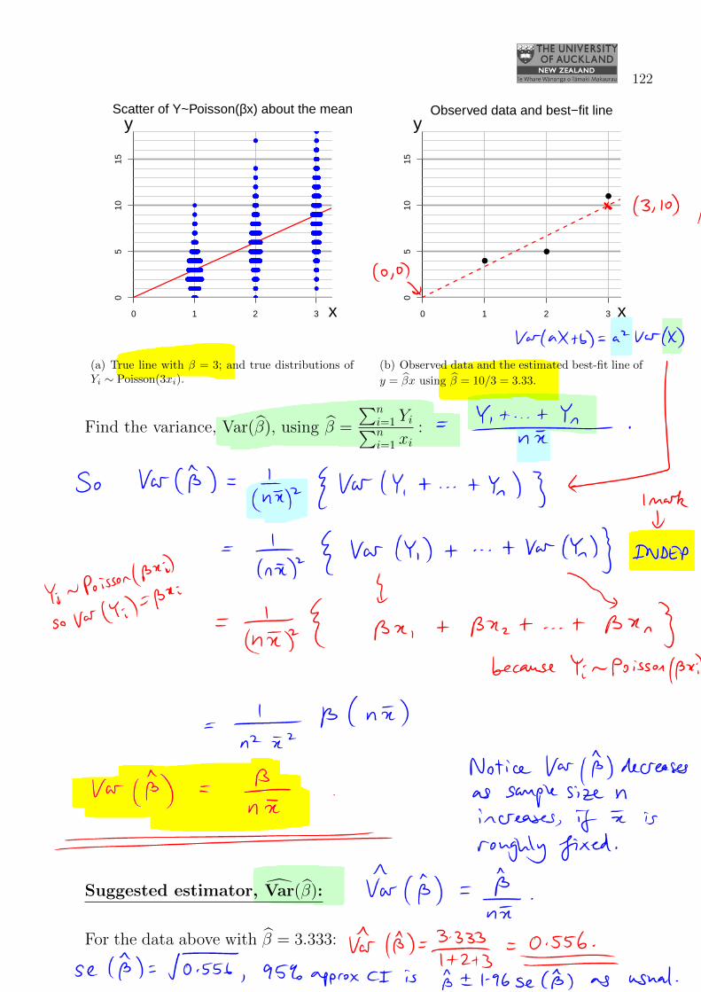
Scatter of Y~Poisson(βx) about the mean
(a) True line with β = 3; and true distributions ofYi ∼ Poisson(3xi).
●
05
1015
0 1 2 3 x
y
●
●
●
Observed data and best−fit line
(b) Observed data and the estimated best-fit line of
y = βx using β = 10/3 = 3.33.
Find the variance, Var(β), using β =
∑ni=1 Yi∑ni=1 xi
:
β =1
nx(Y1 + Y2 + . . .+ Yn)
So Var(β) =
(1
nx
)2 {Var(Y1) + Var(Y2) + . . .+ Var(Yn)
}
by independence of Y1, . . . , Yn
=1
n2 x2 (βx1 + βx2 + . . .+ βxn)
because Yi ∼ Poisson(βxi) so Var(Yi) = βxi
=βnx
n2 x2
=β
nx.
Notice that Var(β) depends upon the unknown true value of β, andthat the variance gets smaller as n increases: large n means largesample sizes, for fixed x.
Suggested estimator, Var(β): Use the obvious one, Var(β) =β
nx.
For the data above with β = 3.333: Var(β) =3.333
1 + 2 + 3=
3.333
6=
5
9= 0.556 .