CHAPTER 3

From Surface to Image

3.1. Introduction

Given a light source, a surface, and an observer, a reflectance model describes the

intensity and spectral composition of the reflected light reaching the observer. The

intensity of the reflected light is determined by the intensity and size of the light

source and by the reflecting ability and surface properties of the surface. In this

chapter, we will discuss the modelling techniques from 3D surface to 2D image.

First all, we introduce surface roughness models, including height distribution model

and slope distribution model, and then the illumination geometry used in this thesis is

illustrated. Secondly, various reflection and illumination modelling is under the

review. Therefore a simple Lambertian illumination model is presented to describe

diffuse reflection. Thirdly, We present the Kube-Pentland’s surface model, a linear

Lambertian model used in this thesis. A deep investigation about this model is given,

with regard to its frequency domain responses, directional filter, effect of non-linear

and shadowing. Fourthly, four models of rough synthetic surfaces are given for the

purpose of simulation process. Finally, we demonstrate that surface rotation

classification is not equivalent to image rotation classification.

3.1.1. Surface Roughness

30

The manner in which light is reflected by a surface is dependent on the shape

characteristics of the surface. In order to analyse the reflection of incident light, we

must know the shape of the reflecting surface. In another words, we need a

mathematical model of the surface. There are two ways to describe the model of

surface and its roughness: the height distribution model and the slope distribution

model [Nayar91]. A brief discussion of existing surface roughness models is given

below, in order to identify significant limitations in currently applied methods.

• Height distribution model

In height distribution model, the height coordinate of the surface may be expressed

as a random function and then the shape of the surface is determined by the

probability distribution of the height coordinates. The usual general measures of

surface roughness are the standard deviation of the surface heights σs (root-mean-

square roughness) and average roughness Rcla (Centre Line Average CLA), which

can be obtained as follows:

[ ]2

1)()(1 ∑

=

−=n

xs xsxs

nσ (3. 1)

∑=

=n

xcla xs

nR

1)(1

(3. 2)

where s(x) presents the height of a surface at a point x along the profile, )(xs is the

expectation of s(x) and n is the number of pixels. Hence, they provide measures of

the average localised surface deviation about a nominal path. The shape or form of

the textural surface cannot be implied from these measures. Indeed textures with

differing physical characteristics may result in similar values [Smith99a]. We also

have to note that the surface roughness cannot be defined by one of these parameters,

either σs or Rcla, since two surfaces with the same height distribution function may

not resemble each other in many cases [Nayar91]. Hence using such a model, it is

difficult to derive a reflectance model for arbitrary source and viewer directions.

31

• Slope distribution model

The slope distribution model is commonly utilised in the analysis of surface

reflection as the scattering of light rays has been shown to be dependent on the local

slope of the surface and not the local height of the surface. The slope model is

therefore more suitable for investigation of the problem of surface reflection. It is

useful to think of a surface as a collection of planar micro-facets, as illustrated in

Figure 3. 1.

Bump map surface

Nominal surfaceSurface normals

L

ε

Figure 3. 1 A surface as a collection of planar micro-facets

If a surface is mathematically smooth and each facet area ε is small compared to the

area L of the surface patch (L >>ε), we may use two slope parameters, prms and qrms,

as a measure of roughness. They correspond to the standard deviation of the surface

partial derivatives p and q.

2

1

),( ),( 1 ∑=

⎟⎟⎠

⎞⎜⎜⎝

⎛∂

∂−

∂∂

=n

xrms x

yxsx

yxsn

p (3. 3)

2

1

),( ),( 1 ∑=

⎟⎟⎠

⎞⎜⎜⎝

⎛∂

∂−

∂∂

=n

xrms y

yxsy

yxsn

q (3. 4)

where x

yxs∂

∂ ),( and y

yxs∂

∂ ),( are surface partial derivatives measured along the x and

y axes respectively. Hence prms and qrms can be used to describe surfaces with both

isotropic and directional roughness.

32

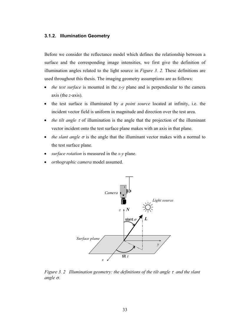
3.1.2. Illumination Geometry

Before we consider the reflectance model which defines the relationship between a

surface and the corresponding image intensities, we first give the definition of

illumination angles related to the light source in Figure 3. 2. These definitions are

used throughout this thesis. The imaging geometry assumptions are as follows:

• the test surface is mounted in the x-y plane and is perpendicular to the camera

axis (the z-axis).

• the test surface is illuminated by a point source located at infinity, i.e. the

incident vector field is uniform in magnitude and direction over the test area.

• the tilt angle τ of illumination is the angle that the projection of the illuminant

vector incident onto the test surface plane makes with an axis in that plane.

• the slant angle σ is the angle that the illuminant vector makes with a normal to

the test surface plane.

• surface rotation is measured in the x-y plane.

• orthographic camera model assumed.

x

y

z

tilt τ

slant σ

Light source

Camera

Surface plane

L

N

Figure 3. 2 Illumination geometry: the definitions of the tilt angle τ and the slant angle σ.

33

3.1.3. Diffuse and Specular

Reflection from smooth surfaces such as mirrors or a still body of water results in a

type of reflection known specular reflection. Reflection from rough surfaces such as

clothing, paper and an asphalt roadway produces a type of reflection known as

diffuse reflection. In practice the reflection process may well be a combination of

both diffuse and specular components. An example of this is a spread reflection,

which has a dominant directional component that is partially diffused by surface

irregularities. Whether the surface is microscopically rough or smooth has a

tremendous impact upon the subsequent reflection of a beam of light. Figure 3. 3

depicts a beam of light incident upon a surface and the resultant reflection for

different types of surfaces. An example of diffuse and specular reflectance for a

sphere is shown in Figure 3. 4.

Specular Diffuse Spread

Figure 3. 3 Specular, diffuse and spread reflection from a surface.

(a) Diffuse (b) Specular

Figure 3. 4 An example of diffuse and specular reflectance.

Several models for the specular component have been proposed. Phong [Phong75]

models a reflection lobe which was spread out around the specular direction by using

a cosine function raised to a power. Blinn [Blinn77] proposed a model which

accounts for off-specular peaks that occur when the incident light is at a grazing

34

angle. These models are relatively simple with regard to calculation and give

reasonably realistic results.

In this thesis, we have to analyse both synthetic and real images, but only the diffuse

reflection is taken into account in general. The specular reflection is simply

disregarded as noise in most cases except for the method proposed in Chapter 9,

where a method based on photometric stereo is developed which is similar to the

approach by Coleman and Jain [Coleman82].

3.2. Reflection and Illumination modelling

The purpose of reflection models in computer vision is to enable the rendering of a

3D surface in 2D space, such that reality is mimicked to a reasonable level. An image

of the surface results from light source reflected from the surface in the direction of

the sensor. The intensity at any given point in the image is closely related to the

reflectance properties of the corresponding point on the surface. Therefore the

prediction or the interpretation of image intensities requires a sound understanding of

the various mechanisms involved in the reflection process.

3.2.1. Review of Related Work

Various reflectance models have been developed in the field of computer vision. In

general they can be classified into two categories: the physical models and the

geometrical models in [Nayar91]. The physicals model use electromagnetic wave

theory to analyse the reflection of incident light. This is more general than the

models based on geometrical optics in that it can describe reflection from smooth to

rough surfaces. However, physical models are often inappropriate for use in machine

vision as they have functional forms which are difficult to manipulate. On the other

hand, geometrical models are derived by analysing the surface and illumination

geometry and have simpler functional forms.

35

L N

V

x

y

Figure 3. 5 The geometry of light reflection.

The geometry of light reflection at a surface is illustrated in Figure 3. 5. Reflection

models are generally presented in terms of a Bidirectional Reflectance Distribution

Function (BRDF). The BRDF is a general model that relates the energy arriving at a

surface from the direction of illumination, to the reflected intensity in the direction of

the viewer:

( )rriiBRDF φθφθλ , , ,, (3. 5)

Where λ is the wavelength of the incident light, (θI , φi) is the direction of the

incoming light and (θr , φr) is the direction of the reflected light shown in Figure 3.

5. The BRDF can be divided into three components: (a) specular component, (b)

directional diffuse component and (c) uniform diffuse component demonstrated in

Figure 3. 6.

36

uniformdiffuse

directionaldiffuse

specular

incidentcone

Figure 3. 6 Three components of BRDF: (1). uniform diffuse component; (2). directional diffuse component and (3). specular component.

Over the past twenty years, a variety of BRDF models of increasing sophistication

have been proposed. He [He91] proposed a general light reflection model that

assumes Gaussian, isotropic rough surface. The model is based on wave optics and

accounts for diffraction and scattering effects. The model provides closed-form

analytical expressions for the specular, directional diffuse and uniform diffuse

components of the BRDF. One paper that does present a method for acquiring

BRDFs is [Ward92]. Ward built an imaging reflectometer that uses the two degrees

of freedom inherent in a camera imaging system to measure BRDFs and presented an

“elliptical Gaussian” model that is capable of modelling certain kinds of anisotropy.

The Lambertian BRDF has enjoyed widespread use for modelling smooth matte

surfaces. The Torrance-Sparrow model [Torrance67] for describing surface reflection

from rough surfaces has been used extensively in computer vision and graphics.

They have appended the Lambertian model to their reflectance model to account for

the internal scattering mechanism. The surface is modelled as a collection of planar

micro facets and the facet slopes are assumed to be normally distributed. Oren and

Nayar [Oren95] derived a reflectance model for matte surfaces which includes local

occlusions, shadowing and interreflections. Work by Wolff [Wolff96] developed a

simple modification of Lambert’s law which accurately accounts for all illumination

and viewing directions. Koenderink and van Doorn [Koenderink96] have measured

the BRDFs for a variety of surfaces. Their measurements indicate they are fairly well

37

behaved and can be represented using a relatively small (50 or less) number of basis

BRDFs.

The most commonly used model in computer vision is the Phong reflection model

[Phong75], which is a linear combination of specular and diffuse reflection. The

specular component is a lobe which spreads out around the specular direction and is

modelled by using a cosine function raised to a power. Phong’s model is usually

given in terms of unit vectors associated with the geometry of the point under

consideration:

( ) ( ) ( )nsidiaa kIkIkInI VRNL ⋅+⋅+=Φ, (3. 6)

where, Ia is the constant intensity of the ambient light;

ka is the coefficient of ambient reflection of the surface;

Ii is the intensity of the incident light;

kd is the coefficient of diffuse reflection for the material;

ks is the coefficient of specular reflection;

Φ is the angle between the mirror vector R and the viewing vector V highlight

shown in Figure 3. 7, and

n is an index that controls the tightness of the specular lobe.

Surface

Φ

Ν

L

V

R

θ θ

Η

Figure 3. 7 Vectors used in the Phong reflection model.

In Phong’s model, the light sources are usually considered as point sources situated

infinitely far away. Hence the angle θ between the incident light and the normal to a

planar surface is constant over the surface. The viewer is assumed to be positioned at

infinity and hence the angle Φ is constant over a planar surface as well. The diffuse

and specular terms are modelled as local components only. Shadows are not

38

considered. The colour of the specular term is assumed to be that of the light source.

Empirical results are used to model the distribution of the specular term around the

reflection vector. It is also important to note that, unlike Lambert’s law, this model

has no physical interpretation; it follows nature in an empirical way only.

Estimating the specular component involves the computation of the reflected vector

R. This is somewhat computationally expensive and hence this is often replaced by

the computation of H, a vector half-way between L and V. This is often called

Blinn’s method [Blinn77]. Therefore H is defined by

2

VLH += (3. 7)

The specular term in Phong’s model then becomes

( )nsispecular kII HN ⋅= (3. 8)

Cook and Torrance [Cook82] extended this model to account for the spectral

composition of highlights – their dependency on material type and the angle of

incidence of the light. These advances have a subtle effect on the size and colour of a

highlight compared to that obtained from the Phong’s model. This model is most

successful in rendering shiny metallic-like surfaces

In the next section, we will discuss the Lambertian illumination model which is used

in this thesis. The Lambertian illumination model is the simplest type of reflection. It

does reasonably well in approximating reflection for a matte surface that looks the

same from all directions. It is widely used in the field of computer vision as a simple

model.

3.2.2. Lambertian Illumination Model

First of all, consider diffuse – optically rough – surfaces reflecting a portion of the

incoming light with radiant intensity uniformly distributed in all directions. A

Lambertian surface will look equally bright from any direction for any illumination

39

direction. In other words, the reflected intensity is independent of the viewing

direction. Examples of such surfaces include cotton cloth, many carpets, matte paper

and matte paints.

However, the intensity does depend on the light source’s orientation relative to the

surface. Mathematically, this is represented as the dot product of the surface

derivative vector with the illuminant vector, and this forms Lambert’s Law.

( )1

cossinsinsincos ),(22 ++

+−=⋅=

qp q -pyxi σστστρλρλ LN (3. 9)

where

• i(x,y) is the image intensity;

• ⎟⎟

⎠

⎞

⎜⎜

⎝

⎛

++++++=

11,

1,

1 222222 qpqp-q

qp-pN is the unit vector normal

to the surface s(x,y) at the point (x,y);

• x

yxsp∂

∂=

),( and y

yxsq∂

∂=

),( are surface partial derivatives measured along

the x and y axes, respectively;

• L = (cosτ ·sinσ, sinσ ·sinτ, cosσ) is the unit vector towards the light source;

• σ and τ are the illuminant vector’s slant and tilt angles defined in Figure 3. 2;

• ρ is surface albedo, a material dependent coefficient;

• and λ is the strength of the light source.

To use Lambertian law we have to make the following assumptions:

1) The surface is ideally diffuse, where the incident light is equally re-distributed in

all directions, and its reflectance function is uniform. The situation where the

surface is non-uniform can be dealt with using ρ and λ.

2) The viewer is far away form the surface relative to the size of test surface, so that

orthographic projection in the image system can be assumed.

3) Light sources are supposed to be infinity from the surface, such that the light

source energy does not depend on the position of the surface. In other words, it

assumes that illumination is constant over the whole surface.

40

4) For a perfect Lambertian model, both self and cast shadows are ignored, as well

as inter-reflections.

5) We only consider the angle of incidence θ from 0 to 90 degrees. Greater angles

(where the N·L is negative) are blocked by the surface and the reflected energy is

0. The light is incident on the back of the surface, meaning it is blocked by the

object.

6) It is obvious that the Lambertian model cannot describe specular reflections, or

highlights, which occur at places where the direction of direct reflection equals

the viewing direction.

The Lambertian model has been shown to describe diffuse reflection reasonably

well. It was used by Woodham [Woodham80] to determine surface shape by using

the photometric stereo. Coleman and Jain [Coleman82] extend photometric stereo to

four light sources, where specular reflections are discarded and estimation of surface

shape can be performed by means of diffuse reflections and the Lambertian model.

Nayar, Ikeuchi and Kanade [Nayar90] developed the photometric approach which

uses a linear combination of Lambertian and an impulse specular component to

obtain the shape and reflectance information for a surface.

3.3. Kube-Pentland Surface Model

Kube and Pentland [Kube88] present a spectral model for the formation of the image

from an illuminated fractal surface. It is shown that the power spectral density is a

function of the illumination angles and therefore extrinsic in nature, while the fractal

dimension on the other hand is purely a function of the original surface and is

therefore an intrinsic texture measure. Therefore, Kube and Pentland’s surface model

will be used in this thesis.

3.3.1. Theory

41

• Assumptions

This theory assumes the following:

1) The surface reflectance is Lambertian;

2) An orthographic camera model;

3) A viewer-centred co-ordinate system, in which the reference plane of the surface

is perpendicular to the viewing direction;

4) Surface albedo is constant.

5) A constant illumination vector over the surface;

6) The illumination vector is not close to the viewing direction;

7) Shadows and specularities are two aspects of real illumination not predicted by

the model;

8) Inter-reflection is not predicted too.

9) The surface slope angles are small and the surface is smoothed sufficiently for it

to be differentiable.

• Kube’s linear reflectance model

Kube and Pentland’s model predicts that the intensity will approximate a linear

combination of the surface derivatives. Now we recall the Lambertian reflectance

model in equation (3. 9), where the image i(x,y) can then be expressed as a function

of the illuminant orientation (τ,σ) and the surface derivative fields, p(x,y) and q(x,y)

where ρλ=1. This results in a non-linear operation at each facet. Taking the

MacLaurin expansion of 1

1 22 ++ qp

in the equation (3. 9) and yields

( ) ( ) ( )⎥⎥⎦

⎤++⎢

⎣

⎡ +−+−−= ...

!49

!21cossinsinsincos,

22222 qpqpqpyxi σστστ (3. 10)

Using the first three terms forms a linear estimate

( ) σστστ cossinsinsincos, +−−= qpyxi (3. 11)

or

42

[ ]⎥⎥⎥

⎦

⎤

⎢⎢⎢

⎣

⎡−−=

1cossinsinsincos q

pI σστστ (3. 12)

where the approximation is reasonable at p>>p2 and q>>q2 (i.e. p and q are small)

so that the quadratic and higher order terms can be neglected. The form of Kube’s

model is optimal in the least squares sense [McGunnigle98]. Chantler reported that

the error introduced by this approximation for a slant angle of 15° is 3.5% in

[Chantler94a]. It is also noted that if the slant angle σ becomes small, sinσ ≈ 0 and

this means that the quadratic terms in equation (3. 10) cannot be neglected. Kube

therefore further assumes sinσ > 0.1, i.e. the illuminant vector L is not within 6° of

the z axis [Kube88].

3.3.2. Frequency Domain Responses

More specifically, an expression for the spectrum of the image is developed in terms

of the surface texture’s spectrum and illuminant vectors. We note that since

differentiation is a linear operation, equation (3. 11) can be transformed into the

frequency domain and expressed as a function of the surface magnitude spectrum

while discarding the constant term [Chantler94a] [McGunnigle98]:

( )I i Sm ( , ) . .sin .cos . ( , )mω θ ω σ θ τ ω θ= − (3. 13)

where

• Im(ω,θ) is the image magnitude spectrum;

• Sm(ω,θ) is the surface magnitude spectrum;

• ω is the angular frequency of the Fourier component;

• θ is its direction with respect to the x-axis;

• i represents a 90° phase shift; and

• σ and τ are the illuminant vector’s slant and tilt angles

This equation can be divided into three components:

1. the surface response ( ) ( )[ ]θω,Sωiθω,I mms ⋅⋅= ;

43

2. the tilt response ( ) ( )[ ]τθcosθ,ωImτ −= ; and

3. the slant response ( ) [ ]sinσθ,ωImσ = .

For the purposes of this thesis it is more helpful to express equation (3. 13) in terms

of the power spectrum:

),()cos(sin),( 222 θωτθσωθω ϕSI −= (3. 14)

where

• (ω,θ) is the polar form of spatial frequency with θ=0° being the direction

of the x-axis;

• I(ω,θ) is the image power spectrum, and

• Sϕ(ω,θ) is the surface power spectrum of a surface orientated at ϕ. Note

that surface orientation ϕ and direction of spectrum θ are on the same

plane x-y with respect to the x-axis.

This equation contains simple trigonometric terms, which enable the directional

effect of illumination to be more easily understood. Since we are interested in surface

rotation, we only deal with the effects of the ( ) 2cos τθ − term, which is a directional

filter and is independent of radial frequency ω.

3.3.3. Directional Filter

• Surface rotation vs. image rotation.

If we consider only the directional aspects of equation (3. 14) we can see that the

image directionality is a product of the illuminant tilt angle τ and the surface

directionality. In this way a surface rotation may not be equivalent to image rotation

if the illuminant is not also rotated. The directionality in the image of a directional

surface is the product of both the surface and illuminant directionalities.

If the surface is an isotopic one, then the surface rotation will have no significant

effect on the image directionality as long as the illuminant direction is held constant.

44

On the other hand, if the surface is a directional one, the surface rotation will alter

the imaged texture beyond simple rotation. This means that a rotated directional

surface is distinctly different in appearance compared to the unrotated surface. Both

of these effects can be seen in Figure 3. 9.

ϕ = 0° ϕ = 90°

ϕ = 0° ϕ = 90°

(a).isotropic

surface

(b).directional

surface

Figure 3. 8 Isotropic surface and directional surface with rotation ϕ=0° and 90° (indicated by the white arrows in the centre). The illuminant tilt is kept constant at τ=0° (indicated by the black arrows in white circles).

• Illumination directional filter.

In equation (3. 13), the most important feature of Kube’s model is the term

( ) ( )[ τθcosθ,ωImτ −= ], which predicts the effect of illumination directional filter in

Kube’s model. This can be understood by considering Figure 3. 8. We may see that,

for an isotropic surface, image directionality is only due to the directional effect of

the illuminant. Therefore, changing the illuminant directions causes a change in the

direction of energy in the corresponding power spectral density (PSD). Furthermore,

the highest texture energy lies in the direction of the illuminant tilt angle τ.

45

tilt angle τ = 0° tilt angle τ = 90°

(a)

(b)

Figure 3. 9 A fractal surface of “rock” rendered by Kube’s model (a). Surfaces at two different illumination directions (tilt angle of τ=0° and τ=90°, indicated by the black arrows in white circles); (b). the corresponding power spectral density.

• Image variance is not a surface rotation invariant feature for directional

surfaces

There is a problem in the case of directional surfaces, where the image variance will

vary with the rotation of the directional surface. Depending on the degree of

directionality, the variation in image variance may cause the classifier to fail. In this

case, the image variance is not a surface rotation invariant feature for directional

surfaces [Chantler94b] [McGunnigle99a].

With regard to the equation (3. 14), the image variance is the integral of the image

power spectrum, assuming the mean component to be equal to zero. The following

can therefore be obtained:

( )∫ ∫∞

⋅−⋅=0 0

2232 ),()(cos2sin)(π

ϕ ωθθωτθσωϕσ ddS (3. 15)

46

If we consider a new axis with the direction of the unidirectional surface texture

where θ* = θ − ϕ , and then equation (3. 15) becomes:

( )∫ ∫∞ −

−

⋅−+⋅=0

***2232 ),()(cos2sin)(ϕπ

ϕϕ ωθθωτϕθσωϕσ ddS (3. 16)

Now if the inner integral part of the equation (3. 16) is taken into account:

[ ]

( ) ( )[ ]∫

∫

∫∫

∫

∫

⋅−⋅+−⋅+

=

⋅−++=

⋅−++=

⋅−+−

−

π

ϕ

π

ϕ

π

ϕ

π

ϕ

π

ϕ

ϕπ

ϕϕ

θθωϕτθϕτθ

θθω

θθωτϕθθθω

θθωτϕθ

θθωτϕθ

0

0

0

***

0

**

0

***

***2

),(22sin2sin22cos2cos

),(

),()222cos( ),(

),()222cos(1

),()(cos2

dS

dS

dSdS

dS

dS

(3. 17)

Therefore equation (3. 15) can be simply expressed in the form of

[ ] [ ][ ])2cos(

)22sin()22cos()(2

φτϕτϕτϕσ

++=−+−+=

DACBA

(3. 18)

where

( )[ ] ϕφ

ωθθωθωσ

ωθθωθωσ

ωθθωωσ

π

ϕ

π

ϕ

π

ϕ

2/arctan

),(2sin)(sin

),(2cos)(sin

),()(sin

22

0 0

32

0 0

32

0 0

32

+=+=

⋅=

⋅=

=

∫ ∫

∫ ∫

∫ ∫

∞

∞

∞

BCCBD

ddSC

ddSB

ddSA

From equation (3. 18), we may note that

47

• for an isotropic surface, the term D will be equal to zero, and then the image

variance σ 2(ϕ) will be kept constant;

• on the other hand, for a directional surface, the term B will not be equal to zero

and therefore image variance σ 2(ϕ) will be a raised cosine function of surface

orientation.

Figure 3. 10 illustrates the variation of image intensity variance with surface rotation

for an isotropic surface “gr2” and a directional surface “wv2” (shown in Figure 3. 8

with the constant illumination tilt angle τ=0°). We may note that the variance of

image intensity for the directional surface “wv2” is certainly not invariant to surface

rotation and indeed it is following the cosine term predicted in the model. It is this

directional filter effect that makes the outputs of texture features vary with the

orientation of a directional surface.

0.0E+00

2.0E+03

4.0E+03

6.0E+03

8.0E+03

1.0E+04

1.2E+04

0° 20° 40° 60° 80° 100° 120° 140° 160° 180°

angle of surface rotation

imag

e va

rianc

e

w v2 (tilt = 0)

gr2 (tilt = 0)

Figure 3. 10 The variation of image intensity variance with surface rotation for an isotropic surface “gr2” and a directional surface “wv2” (illumination tilt angle τ=0°).

3.3.4. Non-linear Effects

In this section, we investigate the non-linear effects occurring in Kube’s image

model through the use of simulation. One of the reasons for this effect, is that the

48

quadratic and higher order terms in equation (3. 10) are neglected in developing the

linear image model in equation (3. 11). Furthermore, the linear image model is based

on the assumption that surface height variance is low (i.e. surface slope is less than

15 degrees) and that the slant angle does not approach 0 degrees. These assumptions

are necessary to allow the Lambertian model to be linearised [Chantler94].

• Surface amplitude variance

The linear image model assumes a linear relationship between the image variance

and surface variance (equation (3. 13)). Figure 3. 11 and Figure 3. 12 show the effect

of increasing the amplitude of a simple sinusoidal surface on images modelled with

perfect Lambertian reflection (equation (3. 9)) and linear Lambertian reflection given

by Kube’s model in equation (3. 11). In order to investigate the effect of the non-

linear components, we set the illumination slant angle σ=45°. This angle was chosen

because the reflection model assumes a cos2 relationship between slant angle σ and

the reflected intensity, and the model seems to be most linear for a slant angle of

around 45°.

49

-5

-4

-3

-2

-1

0

1

2

3

4

5

6

0 2 4 6 8 10 12

x-distance

mag

nitu

de/in

tens

it

14

y

surface Perfect Lambertian linear Lambertian

Surface amplitude = 2

Figure 3. 11 The non-linear effects of a sinusoidal corrugated surface intensity with amplitude=2, predicted by perfect Lambertian model and linear Lambertian model (σ=45°).

-5

-4

-3

-2

-1

0

1

2

3

4

5

6

0 2 4 6 8 10 12

x-distance

mag

nitu

de/in

tens

it

14

y

surface Perfect Lambertian linear Lambertian

Surface amplitude = 4

Figure 3. 12 The non-linear effects of a sinusoidal corrugated surface intensity with amplitude=4, predicted by perfect Lambertian model and linear Lambertian model (σ=45°).

In both Figure 3. 11 and Figure 3. 12, it can be seen that the difference or distortion

between perfect Lambertian surface and a linear Lambertian surface occurs at the

position where the non-linear effects are significant, i.e. where the surface slope

50

angles approach their maximum values. In addition, increasing the surface amplitude

from 2 to 4 accentuates these differences.

Next, we consider the situation where the illumination slant angle σ approaches the

extremes i.e. 0° and 90°, such that the non-linear effect can be investigated further.

• Frequency doubling

For an illumination slant angle close to 0°, where the source of illumination is

vertically above the surface, the equation (3. 10) becomes:

( ) ( )⎥⎥⎦

⎤++⎢

⎣

⎡ +−= ...

!49

!21cos,

22222 qpqpyxi σ (3. 19)

This shows that the effect of the linear term is reduced and the higher order and

quadratic terms now have a greater influence on the image intensity. An example of

the frequency doubling effect of a sinusoidal corrugated surface f(x,y)=sinωx is

shown in Figure 3. 13. It is illuminated at slant angle σ=0°, therefore the intensity

becomes dominated by the “q” term while the “p” term equals zero. This removes

some of the important linear terms and leaves the intensity dependent on the non-

linear term in equation (3. 20)

ωω 2cos1cos2 2 += (3. 20)

This shows the frequency doubling effect caused by increased distortion from the

saturation of the reflection law in the testing at a sinusoidal surface in Figure 3. 13.

• Clipping

On the other hand, if the slant angle σ is increased, the reflected intensity of the

surface becomes further saturated by distortion as it approaches 90°. This effect can

be seen in Figure 3. 14 where the surface is illuminated with the slant angles σ of

from 40° to 80°, respectively. We may see that the clipping effects apparently

become more severe with increasing the slant angle σ, demonstrating the non-

linearity in that region.

51

-5

-4

-3

-2

-1

0

1

2

3

4

5

6

0 2 4 6 8 10 12

x-distance

mag

nitu

de/in

tens

it

14

y

surface

Lambertian

Figure 3. 13 Frequency doubling effect of a sinusoidal corrugated surface illuminated at slant angle σ=0°.

-5

-4

-3

-2

-1

0

1

2

3

4

5

0 2 4 6 8 10 12

x-distance

mag

nitu

de/in

tens

it

14

y

surface Lambertian (slant=40)Lambertian (slant=60) Lambertian (slant=80)

Figure 3. 14 Clipping effect of a sinusoidal corrugated surface illuminated at slant angle σ=40°, 60° and 80°.

52

3.3.5. Effect of Shadowing

Another non-linear contribution to the model is shadowing. One assumption used in

our mathematical equation is Lambertian reflection where shadowing is ignored.

Unfortunately in the real world shadows occur. They account for strong

disagreement with the Lambertian model when real textures are used. This model is,

however, a reasonable approximation of real smooth diffuse reflection given certain

constraints. For a rough surface, it is acknowledged that there are significant

departures from Lambert’s law. Moreover, the departures are most marked for

specific viewer and light source directions. The Lambertian model breaks down

substantially when the angle between the view vector and the surface normal exceeds

60 degrees [Wollf98]. In this section, we will discuss the effect of shadowing on our

model.

• Self shadow and cast shadow

Shadows occur either at places where the path from the light source is blocked or at

surfaces which are oriented away from the light source. These effect known as cast

shadow and self shadow, respectively, and illustrated in Figure 3. 15. The two kinds

of shadows also have quite different properties.

1. The self shadow depends on the relation between the surface normal and the

lighting direction, and it is observed where the surface does not face the lighting

direction.

2. On the other hand, the cast shadow depends on the whole 3D shape of the

surface, and it is observed where the light is occluded by other objects.

53

Light

3D Surface

Self-shadow

Cast-shadow

Non-shadow

Non-shadow

Figure 3. 15 Illustrations of cast shadow and self shadow on a 3D surface.

• Kube’s model rendered by the effect of shadow

In Figure 3. 16, we simulate sinusoidal surfaces rendered by Kube’s model with the

effect of shadow. An approximation to shadowing can be simply modelled in the

following way: where the shadow occurs the reflected intensity is clipped and set to

0. We may clearly see that the distortions caused by the shadowing (either self or

cast shadow) become more distinctive compared to that without the shadowing

effect.

• Directional filtering effect reduces with a decrease in the slant angle σ in the

case of shadow.

As discussed in section 3.3.3 where we considered the directional filtering effect on

Kube’s model and equation (3. 19), we may note that for a slant angle σ decreasing

to near 0°, the effect of the linear term is reduced compared with that of the square or

higher terms. Furthermore the directional filtering effect will be attenuated. Figure 3.

17 shows the effect of decreasing the slant angle σ from 70° to 10°. It is apparent that

the directional filtering effect reduces as the slant angle σ approaches 0°. In addition,

if the surface is rendered with the effect of shadow in Figure 3. 18, the directional

filtering effect with the highest slant angle (i.e. σ =70°) is also be attenuated. In this

case, the heavy shadow effects the linear approximation of Kube’s model, and the

majority of the reflected intensity is clipped to 0.

54

(a)

(c)

(b)

Figure 3. 16 Sinusoidal surfaces rendered by Kube’s model (tilt angle τ=0° and slant angle σ=70°) with the effect of shadow. (a). without any shadow; (b). with self shadow only; (c). with both self and cast shadow.

55

0

0.2

0.4

0.6

0.8

1

0° 30° 60° 90° 120° 150° 180°

surface rotation angle

imag

e va

rianc

e (n

orm

alis

ed) slant10

slant30slant50

slant70

Figure 3. 17 The varation of image intensity variance with surface rotation rendered over a range of illuminant slant angels and without any shadow effect (the surface is sinusoidal one rendered by tilt angle τ=0°).

0

0.2

0.4

0.6

0.8

1

0° 30° 60° 90° 120° 150° 180°

surface rotation angle

imag

e va

rianc

e (n

orm

alis

ed) slant10

slant30slant50

slant70

Figure 3. 18 The varation of image intensity variance with surface rotation rendered over a range of illuminant slant angels and with shadow effect (the surface is sinusoidal one rendered by tilt angle τ=0°).

3.3.6. Summary of Kube-Pentland Model

In this section, we presented Kube and Pentland’s model which predicts that the

intensity approximates a linear combination of the surface derivatives. Furthermore a

frequency-domain model of the image of an illuminated three-dimensional texture is

56

developed in terms of the surface texture’s spectrum and illuminant vectors. Both its

assumptions and theory are summarised. The linear approximation is reasonable at

low surface slope angle.

Firstly, from this theory, the image directionality is a product of the illuminant

direction and surface directionality. As a result, a surface rotation is not equivalent to

an image rotation if the illuminant is not rotated. It also can be seen that the

directional filter characteristics of an image for an isotropic surface are described by

the term of cos(θ − τ). This predicts that the directionality of an image can be

described by a cosine function. In addition, for an isotropic surface, the image

variance will be kept constant; while for a directional surface, the image variance is a

raised power cosine function of surface rotation. Hence we note that image variance

is not a surface rotation invariant feature for a directional surface, which leads to

surface-based classification rather than image-based classification.

Secondly, the non-linear effects neglected by the Kube’s model are considered. Their

effect on surface amplitude variance, frequency doubling and intensity clipping is

investigated through the use of simulation. This confirms Kube’s linear model must

be used on the basis that surface height variance is low and that the slant angle does

not approach 0 degrees.

Lastly, the shadowing contribution to the model is shown, as shadowing can not be

ignored in the real world.

3.4. Descriptions of Synthetic Surface

In this section, we briefly introduce four models of rough synthetic surfaces, which

are used in the whole of this thesis for the purpose of simulation.

If we consider a texture to be a realisation of a two dimensional random process the

texture can be described by its mean and its phase. For a structured surface, there is

57

important information in its phase spectrum. However for unstructured surfaces the

phase spectrum is assumed to be equally distributed. In this thesis, we only deal with

unstructured synthetic surfaces so that the phase spectrum is neglected.

In texture analysis, the fractal model is one of the most commonly used: the texture

is viewed as the realisation of a random process. To characterise the texture, the

fractal dimension has to be estimated. A fractal function is good for modelling 3D

real surfaces because many physical processes produce a fractal surface shape.

Indeed fractals are widely used as a graphics tool for generating natural-looking

shapes. A survey of natural imagery has shown that the 3D fractal surface model

furnishes an accurate description of both texture and shaded image regions

[Pentland88].

Four surface models have been proposed that are defined in terms of the power

spectrum. They are the 2D forms of the fractal [Pentland88], Mulvanney

[Mulvanney89], Ogilvey [Sayles78] and sand ripple [Linnett91], where the fractal

and Mulvanney surface are isotropic, while the Ogilvey and sand ripple are

directional ones. They are defined as follow:

• Fractal

( ) 3ωω rock

FractalkS = (3. 21)

where S(ω) is two dimensional power spectrum; ω is the radial frequency and krock is

a constant.

• Mulvanney

( )

2/3

2

2

1−

⎟⎟⎠

⎞⎜⎜⎝

⎛+=

cmalvMulvanney kS

ωωω (3. 22)

where ωc is the cut-off frequency and kmalv is a constant.

• Ogilvey

( ) ( )( )2222,

vvuuk

vuScc

ogilOgilvey ++

= (3. 23)

where u and v are Cartesian frequency coordinates; uc and vc are cut-off frequencies

in the x and y directions and kogil is a constant.

58

• Sand ripple

( )( ) ( )

322

,

⎥⎦⎤

⎢⎣⎡ −+−

=

dc

sandsand

vu

kvuSωω

(3. 24)

where u and v are Cartesian frequency coordinates; ωc and ωd are cut-off frequencies

in the x and y directions and ksand is a constant.

Images of these surfaces rendered with the Lambertian model are shown in Figure 3.

19. Note that in the rest of this thesis, we denote fractal surface as “rock”,

Mulvanney surface as “malv”, Ogilvey surface as “ogil” and sand ripple as “sand”.

(a). Fractal

(d). Sand ripple

(c). Ogilvey

(b). Mulvanney

Rendered surface PSD

Figure 3. 19 Four synthetic textures rendered with a Lambertian model and their corresponding surface height PSD.

59

3.5. Image-based Classification vs. Surface-based Classification

Many texture classification schemes have been presented that are invariant to image

rotation [Port97a] [Cohen91] [Mao92]. They normally derive their features directly

from a single image and are tested using rotated images. If the image texture results

solely from albedo variation rather that surface relief or if the illumination is not

directional or immediately overhead, then these schemes are surface-rotation

invariant as well. However, in many cases rotation of a textured surface produces

images that differ radically from those provided by pure image rotation (an example

can be seen in Figure 3. 8). This is mainly due to the directional filtering effect of

imaging using side-lighting, described by Kube’s frequency model in equation (3.

13). Therefore, a distinction between classifying a surface using measured pixel

intensities and classifying on the basis of the reflectance function is apparent.

Kube and Pentland [Kube84] identified and verified a frequency domain model of

the image formation process for 3D surface texture. This has shown that the imaging

process acts as a directional filter of texture and that changes in illuminant direction

can cause catastrophic failure of classifiers [Chantler94b] [McGunnigle98]. Chantler

[Chantler94] has used Kube’s model to remove the directional effect associated with

illumination in his scheme which estimates a quantity that is independent of the

orientation of the surface and relative to the illuminant. However, there are two main

weaknesses that stem from the linearization of Kube’s model. The scheme is firstly

unable to deal with the situation where the surface normal is perpendicular to

illuminant direction. Secondly, only some classes of surfaces are suitable to the use

of a linear model. Based on these reasons, this theme is not sufficiently robust with

regard to the rotation of texture. However a new methodology [McGunnigle00] was

developed for texture classification based on the direct use of surface gradient and

surface reflectance information which used photometric stereo to extract and separate

surface relief and albedo information. This enables classification to be performed by

comparing texture features computed directly from surface properties rather than

image intensity values.

60

An example of classification accuracy for image rotation and surface rotation is

given in Figure 3. 20. The statistical classifier is used on a set of isotropic Gabor

filters where the features contain no information about the directionality of the

texture so that they are rotation insensitive features. The detailed structure of the

rotation insensitive classifier can be found in [McGunnigle99a]. The four synthetic

test textures used in this experiment are described in the previous section of this

chapter. First of all, the image is rotated and then the conventional rotation invariant

algorithms are tested. Secondly, the surface is rotated and rendered by Kube’s model

under the same illuminant condition. From the classification accuracy in Figure 3.

20, we may see that the conventional rotation invariant algorithms are not able to

deal with the surface rotation compared to those utilising image rotation. In our

experiments with data sets at surface rotation ϕ=0°, the prominent directionality of

the surface is perpendicular to the illuminant direction. Therefore at surface rotation

ϕ=90°, surface directionality and illuminant direction are the same. This effect

makes the discrimination more difficult and the classification accuracy was found to

decrease significantly. This again demonstrates that surface rotation is not equivalent

to image rotation for 3D surfaces.

40

50

60

70

80

90

100

0° 30° 60° 90° 120° 150° 180°

angle of rotation

clas

sific

atio

n ac

cura

cy (%

)

Image RotationSurface Rotation

Figure 3. 20 Classification accuracy for image rotation and surface rotation.

61

3.6. Summary

In this chapter, the process from surface to image is reviewed. First of all, the surface

roughness models were discussed, illumination geometry defined and diffuse and

specular reflectance were considered. A review of related work on reflection and

illumination modelling was given. Afterwards, a simple Lambertian illumination

model was selected. It is proven to describe diffuse reflection reasonably well.

We presented Kube’s model, a linear Lambertian model, which assumes fixed

illumination and viewing geometry and expresses observed intensity as a linear

function of surface partial derivatives. We model all the surfaces as Lambertian.

Most of the surfaces have moderate slopes and can be accurately rendered using a

linear approximation. From this model, one characteristic of rough surface textures is

that the appearance of the surface is a function of the illuminant direction as well as

of the surface topography. Furthermore, Kube’s model functions as a directional

filter. In addition, the non-linear effects neglected by the model were investigated.

With regard to surface amplitude variance, they are frequency doubling and intensity

clipping. Finally the shadowing contribution to the model was also shown.

We briefly introduced four models of rough synthetic surfaces, which are used in the

throughout this thesis for the purpose of simulation. They are the 2D forms of the

fractal, Mulvanney, Ogilvey and sand ripple.

We demonstrated that the rotation of a directional surface is not equivalent to the

rotation of its image. Therefore a surface rotation invariant classifier must take this

effect into account. One approach is to classify using the properties of the surface

rather than those of the image. If the properties of the surface can be estimated, it

may be possible to improve the performance of the classifier. We will introduce the

photometric stereo technique in the next chapter, which will enable us to directly

estimate surface properties from several images illuminated under different lighting

sources.

62