Embed Size (px)
Citation preview

Affected Environment
Chapter 3
3.1 Introduction 3.2 Land Ownership and Use 3.3 Air Quality 3.4 Geology, Soils, and Erosional
Processes 3.5 Water Resources 3.6 Vegetation 3.7 Riparian and Wetland Processes 3.8 Fish and Fish Habitat 3.9 Amphibians and Amphibian
Habitat 3.10 Birds, Mammals, Other Wildlife,
and Their Habitats 3.11 Recreation 3.12 Visual Resources 3.13 Archaeological, Historical,
Cultural and Indian Trust Resources
3.14 Social and Economic Environment


Final EIS Introduction
Chapter 3
3-1
3. AFFECTED ENVIRONMENT 1
2
3.AFFECTED ENVIRONMENT ............................................................................................. 3-1 3 3.1 INTRODUCTION ...................................................................................................... 3-2 4 3.2 LAND OWNERSHIP AND USE................................................................................ 3-5 5
3.2.1 Introduction .................................................................................................. 3-5 6 3.2.2 Existing Habitat Conservation Plans............................................................ 3-9 7 3.2.3 Land Ownership and Use by Region ........................................................... 3-9 8 3.2.4 Timber Harvest for Western and Eastern Washington .............................. 3-13 9 3.2.5 Forestland Conversion............................................................................... 3-19 10
3.3 AIR QUALITY ......................................................................................................... 3-25 11 3.4 GEOLOGY, SOILS, AND EROSIONAL PROCESSES.......................................... 3-27 12
3.4.1 Geology and Soils...................................................................................... 3-27 13 3.4.2 Erosion ....................................................................................................... 3-30 14
3.5 WATER RESOURCES........................................................................................... 3-39 15 3.5.1 Surface Water Quality................................................................................ 3-39 16 3.5.2 Surface Water Quantity.............................................................................. 3-45 17 3.5.3 Groundwater Quantity and Quality ............................................................ 3-53 18
3.6 VEGETATION......................................................................................................... 3-55 19 3.6.1 Forest Vegetation....................................................................................... 3-55 20 3.6.2 Riparian Vegetation ................................................................................... 3-60 21 3.6.3 Disturbance Agents.................................................................................... 3-61 22 3.6.4 Threatened and Endangered Plants.......................................................... 3-65 23 3.6.5 Invasive Plants........................................................................................... 3-65 24
3.7 RIPARIAN AND WETLAND PROCESSES............................................................ 3-67 25 3.7.1 Riparian Areas ........................................................................................... 3-67 26 3.7.2 Wetlands .................................................................................................... 3-73 27
3.8 FISH AND FISH HABITAT...................................................................................... 3-79 28 3.8.1 Introduction ................................................................................................ 3-79 29 3.8.2 Fish Status in Washington ......................................................................... 3-79 30 3.8.3 Life History of Covered and Affected Fish Species ................................... 3-80 31 3.8.4 The Freshwater Aquatic Ecosystem .......................................................... 3-96 32 3.8.5 Fish and Fish Habitat by Analysis Region ............................................... 3-104 33
3.9 AMPHIBIANS AND AMPHIBIAN HABITAT.......................................................... 3-113 34 3.9.1 Introduction .............................................................................................. 3-113 35 3.9.2 Amphibian Distribution, Status, and Habitat ............................................ 3-114 36 3.9.3 Review of Timber Harvest Effects on Amphibians................................... 3-120 37
3.10 BIRDS, MAMMALS, OTHER WILDLIFE AND THEIR HABITATS....................... 3-125 38 3.10.1 Introduction .............................................................................................. 3-125 39 3.10.2 Federally Threatened or Endangered Wildlife Species ........................... 3-127 40 3.10.3 Importance of Riparian Habitats to Wildlife.............................................. 3-135 41 3.10.4 Wildlife in Upland Forested Habitats........................................................ 3-137 42

Introduction Final EIS
Chapter 3
3-2
3.11 RECREATION.......................................................................................................3-141 1 3.11.1 Introduction ...............................................................................................3-141 2 3.11.2 Estimates of Future Recreational Needs..................................................3-142 3 3.11.3 Private Lands and Recreation ..................................................................3-143 4 3.11.4 Forest Road-related Recreation ...............................................................3-143 5
3.12 VISUAL RESOURCES..........................................................................................3-145 6 3.12.1 Introduction ...............................................................................................3-145 7 3.12.2 Visual Resources and the Current Washington Forest Practices Rules ..3-147 8
3.13 ARCHAEOLOGICAL, HISTORICAL, CULTURAL AND INDIAN TRUST 9 RESOURCES........................................................................................................3-149 10 3.13.1 Introduction ...............................................................................................3-149 11 3.13.2 Archaeological Overview ..........................................................................3-149 12 3.13.3 Cultural and Trust Resources of Native American Tribes ........................3-152 13 3.13.4 Overview of Regional History ...................................................................3-154 14 3.13.5 Washington State Protective Structure.....................................................3-155 15
3.14 SOCIAL AND ECONOMIC ENVIRONMENT ........................................................3-157 16 3.14.1 Introduction ...............................................................................................3-157 17 3.14.2 Population.................................................................................................3-157 18 3.14.3 Employment and the Economy.................................................................3-158 19 3.14.4 Environmental Justice ..............................................................................3-165 20
21
3.1 INTRODUCTION 22 This chapter describes the affected environment to provide background for the assessment 23 of the environmental effects of the alternatives in Chapter 4 (Environmental Effects) and 24 Chapter 5 (Cumulative Effects). The affected environment sections describe the resources 25 and their current conditions against which the anticipated environmental effects of the 26 alternatives described in Chapter 2 (Alternatives) are evaluated. The first section describes 27 land ownership and use within the State, to provide context for the description of the other 28 sections. The remaining sections present the physical environment first, followed by the 29 biological environment, and then the social environment. The specific order of the sections 30 is as follows: 31
• Land Ownership and Use (subsection 3.2) 32 • Air Quality (subsection 3.3) 33 • Geology, Soils, and Erosional Processes (subsection 3.4) 34 • Water Resources (subsection 3.5) 35 • Vegetation (subsection 3.6) 36 • Riparian and Wetland Processes (subsection 3.7) 37 • Fish and Fish Habitat (subsection 3.8) 38 • Amphibians and Amphibian Habitat (subsection 3.9) 39 • Birds, Mammals, Other Wildlife and Their Habitats (subsection 3.10) 40 • Recreation (subsection 3.11) 41 • Visual Resources (subsection 3.12) 42 • Cultural Resources and Indian Trust Resources (subsection 3.13) 43 • Socioeconomic Conditions (subsection 3.14) 44

Final EIS Introduction
Chapter 3
3-3
The study area that defines the affected environment includes the majority of the State of 1 Washington. The proposed action and the alternatives would directly affect the forested 2 lands that are covered by the Washington Forest Practices Rules. These lands include the 3 non-Federal and non-tribal forestlands of the State (Figure 3-1). These lands are referred 4 to as the “covered lands” or the lands subject to Washington Forest Practices Rules in this 5 EIS (See also the SEPA Final EIS on Alternatives for Forest Practices Rules for: Aquatic 6 and Riparian Resources dated April 2001, Washington Forest Practices Board). 7
In addition to displaying the covered lands, Figure 3-1 displays 12 analysis regions, which 8 are similar to the 10 regions identified in the Forest Practices Alternatives SEPA EIS Rules 9 for Aquatic and Riparian Resources (Washington Forest Practices Board 2001c, 2002). 10 However, to more fully capture the diverse landscape of the Puget Sound Region, this 11 Region was divided into three smaller regions in this document. Detailed maps of each 12 analysis region that illustrate rivers, lakes, highways, and more local place names are 13 provided in the Regional Summaries (DEIS Appendix A). 14
The 12 analysis regions are referenced in this EIS to describe some of the regional aspects 15 of the affected environment. This information is used in Chapters 4 and 5 to assess the 16 indirect effects of the alternatives described in Chapter 2 (Alternatives). The regions were 17 defined based on three factors: the distribution of threatened and endangered salmonids, 18 Water Resource Inventory Area (WRIA) boundaries, and the physiographic regions of the 19 State. The 12 analysis regions consist of 7 western Washington regions and 5 in eastern 20 Washington as follows: 21
Western Washington Analysis Regions 22
• North Puget Sound 23 • South Puget Sound 24 • West Puget Sound 25 • Islands 26 • Olympic Coast 27 • Southwest 28 • Lower Columbia 29 Eastern Washington Analysis Regions 30
• Middle Columbia 31 • Upper Columbia – Downstream of Grand Coulee Dam 32 • Upper Columbia – Upstream of Grand Coulee Dam 33 • Snake River 34 • Columbia Basin 35 To provide further background and detail for the affected environment descriptions and the 36 evaluation of effects, detailed summaries of land ownership and use and physical and 37 biological factors were developed for each of the analysis regions. These descriptions are 38 provided in DEIS Appendix A. 39
40

Introduction Final EIS
Chapter 3
3-4
Figure 3-1. Analysis Regions and Covered Lands in Washington.
Figure 3-1. Analysis Regions and Covered Lands in Washington1
1Lands managed under existing HCPs are shown along with covered lands. These lands are not part of the FPHCP. See FPHCP Section 1-5 for a detailed description of HPHCP covered lands.
Final EIS Land Ownership and Use
Chapter 3
3-5
3.2 LAND OWNERSHIP AND USE 1
3.2.1 Introduction 2 The State of Washington is approximately 43,272,000 acres in size. Federal lands 3 comprise approximately 30 percent of the State, with slightly more than one-third of these 4 lands (11 percent of the State) classified as wilderness, national parks, or wildlife refuges. 5 State and tribal lands comprise approximately 9 percent and 7 percent of the State, 6 respectively, with county and city lands accounting for approximately 1 percent. The 7 remaining 53 percent of the lands in Washington are in private ownership (Table 3-1). 8
Slightly more than half of Washington State (53 percent) is forested (Table 3-2). 9 Forestland accounts for 83 percent of western Washington and just 36 percent of eastern 10 Washington. Eastern Washington is, however, considerably larger than western 11 Washington, accounting for 64 percent of the State. Approximately 9 million acres in 12 eastern Washington are forested, compared to 13 million acres in western Washington. 13 Shrubland and grassland comprise approximately 23 percent of the State, with the majority 14 of these lands (97 percent) located in eastern Washington. Agricultural lands account for 15 approximately 18 percent of the State. Freshwater and wetlands account for 2 percent of 16 the State; ice, snow, and bare rock account for another 2 percent; with residential and 17 commercial lands covering the remaining 2 percent (Table 3-2). 18
Approximately 28 percent of forestlands in the State are Federal and State lands not 19 managed for timber production. Federal and tribal lands available for timber management 20 comprise approximately 22 percent of the forestland in the State. The remaining 50 21 percent are State, county, city, and private lands that are potentially available for timber 22 management under the Washington Forest Practices Rules (Table 3-3). These State, 23 county, city, and private lands account for approximately 26 percent of total State lands. 24 State, county, city, and private lands potentially available for timber management under the 25 Washington Forest Practices Rules account for approximately 62 percent of forestlands in 26 western Washington and 34 percent in eastern Washington (Table 3-3). 27
Land ownership and use across Washington State is heavily affected by the distribution 28 and size of the human population. Approximately 5.9 million people resided in 29 Washington State in 2000, an increase of approximately 21 percent or one million people 30 since 1990 (U.S. Census Bureau 2000). Population projections anticipate continued 31 population growth in the State, with the total population projected to reach 7.5 million by 32 2020 (Washington Office of Financial Management 2002a). As the population of the State 33 continues to increase, land ownership and land use are affected, and development in the 34 form of urban growth and low-density residential areas is likely to continue to encroach on 35 the State’s forestlands, farmlands, and fish and wildlife habitat. Population trends are 36 discussed further in subsection 3.14 (Social and Economic Environment). 37
The remainder of this section is divided into four subsections that address existing Habitat 38 Conservation Plans (HCPs), land ownership and use by region, timber harvest rates, and 39 forestland conversion, respectively. 40

Land Ownership and Use Final EIS
Chapter 3
3-6
Table 3-1. Land Ownership Acreage in Washington State by Analysis Region.
Analysis Region
Federal Wildernesses,
National Parks, and Wildlife Refuges
Other Federal Lands
State Parks and Wildlife
Areas
Washington DNR and
Other State Lands
County and City Lands Tribal Lands Private Lands Total
Western Washington North Puget Sound 1,323,585 987,699 20,707 493,568 31,761 40,785 1,499,857 4,397,962 South Puget Sound 200,046 279,906 8,003 161,563 122,175 23,351 1,383,184 2,178,228 West Puget Sound 454,466 235,362 13,154 176,166 9,194 15,349 831,597 1,735,288 Islands 1,990 8,425 11,417 12,895 1,321 0 210,775 246,822 Olympic Coast 529,794 196,674 1,673 309,147 7,752 234,990 476,837 1,756,868 Southwest 12,132 124,872 12,582 304,062 40,062 4,623 1,814,921 2,313,254 Lower Columbia 327,355 750,238 14,033 325,013 2,512 95 1,653,166 3,072,412 Western Washington Total 2,849,368 2,583,176 81,569 1,782,414 214,777 319,193 7,870,337 15,700,834 Percent of Western Washington Total 18% 16% 1% 11% 1% 2% 50% 100%
Eastern Washington Middle Columbia 355,338 1,302,933 178,826 464,006 1,388 1,255,467 2,939,158 6,497,115 Upper Columbia - Downstream of Grand Coulee 1,203,796 2,043,164 183,062 573,642 1,237 431,539 1,964,137 6,400,577 Upper Columbia - Upstream of Grand Coulee 82,706 1,477,635 33,649 345,066 10,293 1,084,900 2,713,551 5,747,801 Snake River 125,263 338,433 44,592 231,230 795 0 3,835,556 4,575,868 Columbia Basin 34,358 353,942 65,990 254,332 214 0 3,641,362 4,350,198 Eastern Washington Total 1,801,461 5,516,107 506,119 1,868,276 13,927 2,771,906 15,093,764 27,571,559 Percent of Eastern Washington Total 7% 20% 2% 7% 0% 10% 55% 100% STATE TOTAL 4,650,830 8,099,284 587,687 3,650,689 228,705 3,091,098 22,964,102 43,272,394 State Total Percent 11% 19% 1% 8% 1% 7% 53% 100% Source: Washington DNR Major Public Lands and WRIA GIS layers 2004.

Final EIS Land Ownership and Use
Chapter 3
3-7
Table 3-2. Acreage of Washington State in General Land Cover/Use Categories by Analysis Region. THE FOLLOWING TABLE REFLECTS SLIGHT CORRECTIONS TO THE NUMBERS
Region Forestland Shrubland Grassland Water and Wetlands
Ice, Snow, and Bare Rock
Residential and Commercial Agricultural Total
Western Washington North Puget Sound 3,427,389 106,174 133,094 70,315 273,175 84,006 303,810 4,397,962 South Puget Sound 1,532,444 32,300 30,042 58,902 47,483 362,597 114,460 2,178,228 West Puget Sound 1,522,197 19,653 22,516 20,668 32,629 71,238 46,387 1,735,288 Islands 180,280 4,246 2,120 2,625 1,809 14,405 41,338 246,822 Olympic Coast 1,671,071 11,469 6,991 33,691 27,081 2,023 4,542 1,756,869 Southwest 2,057,847 16,384 8,708 17,393 37,705 30,949 144,267 2,313,254 Lower Columbia 2,615,716 45,965 24,033 90,245 58,791 65,890 171,772 3,072,412 Western Washington Total 13,006,945 236,191 227,504 293,838 478,673 631,108 826,576 15,700,835 Percent of Western Washington Total 83% 2% 1% 2% 3% 4% 5% 100%
Eastern Washington Middle Columbia 2,691,428 1,828,019 620,489 92,672 52,850 76,321 1,135,336 6,497,115 Upper Columbia-Downstream of Grand Coulee 2,773,963 1,633,425 1,113,611 125,284 153,691 30,129 570,474 6,400,577 Upper Columbia-Upstream of Grand Coulee 4,084,042 360,940 386,508 131,279 3,354 81,353 700,325 5,747,801 Snake River 376,314 1,343,586 369,788 63,443 913 30,921 2,390,903 4,575,868 Columbia Basin 12,843 1,696,447 175,867 111,579 874 46,574 2,306,015 4,350,198 Eastern Washington Total 9,938,590 6,862,417 2,666,262 524,257 211,682 265,298 7,103,053 27,571,559 Percent of Eastern Washington Total 36% 25% 10% 2% 1% 1% 26% 100% STATE TOTAL 22,945,535 7,098,609 2,893,766 818,095 690,355 896,406 7,929,629 43,272,394 Percent of State Total 53% 16% 7% 2% 2% 2% 18% 100% Source: U.S. Geological Survey Land Use/Land Cover and WRIA GIS layers 2004.

Land Ownership and Use Final EIS
Chapter 3
3-8
Table 3-3. Ownership and Management of Forestlands in Washington State by Analysis Region. Forestlands Available for Timber Management and
Subject to Washington Forest Practices Rules
Region
Federal and State Protected Lands Not Managed for
Timber Production1/
Federal and Tribal Lands Available
for Timber Management2/
Washington DNR and Other State Lands3/
Private, County, and City Lands Total
Total Forested
Lands Western Washington
North Puget Sound 1,644,519 235,028 472,932 1,074,910 1,547,842 3,427,389 South Puget Sound 291,193 122,903 148,349 970,000 1,118,349 1,532,444 West Puget Sound 631,196 22,105 168,691 700,204 868,896 1,522,198 Islands 11,706 3,607 10,562 154,405 164,967 180,280 Olympic Coast 684,287 228,828 307,170 450,786 757,957 1,671,071 Southwest 140,690 3,933 294,684 1,618,539 1,913,223 2,057,847 Lower Columbia 719,253 262,482 313,523 1,320,459 1,633,982 2,615,716 Western Washington Total 4,122,844 878,886 1,715,911 6,289,303 8,005,216 13,006,945 Percent of Western Washington Total 32% 7% 13% 48% 62% 100%
Eastern Washington Middle Columbia 879,862 867,469 231,650 712,447 944,097 2,691,428 Upper Columbia-Downstream of Grand Coulee 1,267,217 1,034,605 214,305 257,835 472,140 2,773,963 Upper Columbia-Upstream of Grand Coulee 102,588 2,177,129 284,808 1,519,518 1,804,326 4,084,043 Snake River 95,725 149,067 12,791 118,730 131,522 376,314 Columbia Basin 36 120 1,481 11,205 12,687 12,843 Eastern Washington Total 2,345,428 4,228,390 745,035 2,619,735 3,364,772 9,938,591 Percent of Eastern Washington Total 24% 43% 7% 26% 34% 100% STATE TOTAL 6,468,273 5,107,277 2,460,947 8,909,039 11,369,986 22,945,536 Percent of State Total 28% 22% 11% 39% 50% 100% 1/ Federal and State Protected Lands not Managed for Timber Production includes forestlands set aside for wilderness, late successional reserves, managed late successional reserves, adaptive management
areas, national wildlife refuges, national parks, Washington State parks, and Washington Department of Fish and Wildlife lands. 2/ Federal and Tribal Lands Available for Timber Management include U.S. Forest Service Matrix lands, other National Forest Service lands, BLM lands, Department of Defense lands, and all tribal lands. 3/ Washington DNR and Other State Lands include all Washington DNR, Department of Corrections, and University lands.
Source: U.S. Geological Survey Land Use/Land Cover and WRIA GIS layers 2004

Final EIS Land Ownership and Use
Chapter 3
3-9
3.2.2 Existing Habitat Conservation Plans 1 As of June 2004, there were 11 HCPs in the State of Washington that had been approved 2 by the Services (Table 3-4). Although the specific activities covered and the mitigation 3 requirements vary under each plan depending on the interests of the landowners, most were 4 developed for forest management activities. The only exception to this is the Daybreak 5 Mine HCP, which covers floodplain-adjacent mining. The largest HCP, completed in 6 1997, covers approximately 1.6 million acres of State trust lands managed by Washington 7 DNR. 8
3.2.3 Land Ownership and Use by Region 9 The amount of forestland by region ranges from approximately 13,000 acres in the 10 Columbia River Basin analysis region to just over 4 million acres in the Upper Columbia – 11 Upstream of Grand Coulee Region (Table 3-2). Land ownership and use is summarized by 12 analysis region in Tables 3-1, 3-2, and 3-3 and discussed in the following subsections. 13 More detailed descriptions are found in the Region Descriptions in DEIS Appendix A. The 14
Table 3-4. Completed Habitat Conservation Plans in Washington State (as of 15 October 2004). 16
Name Species Approximate
HCP Start Date1/ Status Acres2/ West Fork Timber 3/ Spotted Owl 1992 Completed 1993 53,500 West Fork Timber All Species 1994 Completed 1995 See Above Scofield Spotted Owl 1996 Completed 1996 4/ 40 Plum Creek (Cascades) All Vertebrates 1993 Completed 1996 170,000 Port Blakely (Robert B. Eddy)
All Species 1994 Completed 1996 7,500
Washington DNR State Trust Lands
All Species6/ 1993 Completed 1997 1,600,0006/
Seattle Public Utilities Multiple Species 1994 Completed 2000 91,000 Green Diamond Resource Co.5/
Multiple Species 1997 Completed 2000 262,000
City of Tacoma/Tacoma Water
Multiple Species 1997 Completed 2001 15,000
Boise Cascade Spotted Owl 2001 Completed 2001 620 Day Break Mine (Storehdahl)
Aquatic Species 1999 Completed 2004 300
1/ Start dates are approximate. Applicants often prepare in advance of initiating active involvement with the Services. 2/ Acres presented here are rounded from acres reported in the original HCP documents. In some cases, lands have been added to
or subtracted from that reported in the original documents, and actual acres managed presently under the HCPs may be slightly different.
3/ Previously known as the Murray-Pacific Corporation; name was changed to the original company name. 4/ The original documents were completed in 1996. However, unlike the other completed HCPs, this resulted in a short-term (1
year) permit, which has since expired. The mitigation continues in the form of a perpetual deed restriction. 5/ Previously known as the Simpson Resource Company. 6/ Aquatic species are not covered on approximately 228,000 acres of State lands on the eastside of the Cascade Crest. Source: USFWS 2004a.

Land Ownership and Use Final EIS
Chapter 3
3-10
analysis regions are shown in Figure 3-1, which also identifies those forestlands that are 1 subject to the Washington Forest Practices Rules. 2
3.2.3.1 Western Washington 3 North Puget Sound 4 The North Puget Sound Region is approximately 4,398,000 acres in size. Approximately 5 3,427,000 acres, or 78 percent, of this area is forestland. Agricultural lands make up 7 6 percent of the Region, and residential and commercial land uses make up 2 percent. 7 Ice/snow and bare rock makes up 6 percent. Other land use/land cover types each make up 8 3 percent or less (Table 3-2). 9
Approximately 48 percent of the forestlands in this Region are managed under a Federal or 10 State protected status that generally does not allow timber production. Approximately 7 11 percent of the forestlands are under other Federal or tribal management and are potentially 12 available for timber production; the remaining 45 percent of the forestlands are State, 13 county, city, and private lands that are potentially available for timber management under 14 the Washington Forest Practices Rules (Table 3-3). 15
South Puget Sound 16 The South Puget Sound Region is approximately 2,178,000 acres in size. Approximately 17 1,532,000 acres, or 70 percent, of this area is forestland. Developed residential and 18 commercial lands make up 17 percent of the Region (primarily the Seattle-Tacoma area), 19 and agricultural lands make up 5 percent. Other land use/land cover types each make up 3 20 percent or less (Table 3-2). 21
Approximately 19 percent of the forestlands in the Region are managed under a Federal or 22 State protected status that generally does not allow timber production. Approximately 8 23 percent of the forestlands are under other Federal or tribal management and are potentially 24 available for timber production; the remaining 73 percent of the forestlands are State, 25 county, city, and private lands that are potentially available for timber management under 26 the Washington Forest Practices Rules (Table 3-3). 27
West Puget Sound 28 The West Puget Sound Region is approximately 1,735,000 acres in size. Approximately 29 1,522,000 acres, or 88 percent, of this area is forestland. Developed residential and 30 commercial lands make up 4 percent of the Region, and agricultural lands make up 3 31 percent. Other land use/land cover types each make up 2 percent or less (Table 3-2). 32
Approximately 41 percent of the forestlands in the Region are managed under a Federal or 33 State protected status that generally does not allow timber production. Approximately 1 34 percent of the forestlands are under other Federal or tribal management and are potentially 35 available for timber production; the remaining 57 percent of the forestlands are State, 36 county, city, and private lands that are available for timber management under the 37 Washington Forest Practices Rules (Table 3-3). 38

Final EIS Land Ownership and Use
Chapter 3
3-11
Islands 1 The Islands Region is approximately 247,000 acres in size. Approximately 180,000 acres, 2 or 73 percent, of this area is forestland. Agricultural lands make up 17 percent of the 3 Region, and developed residential and commercial lands make up 6 percent. Other land 4 use/land cover types each make up 2 percent or less (Table 3-2). 5
Approximately 6 percent of the forestlands in this Region are managed under a Federal or 6 State protected status that generally does not allow timber production. Approximately 2 7 percent of the forestlands are under other Federal or tribal management and are potentially 8 available for timber production; the remaining 92 percent of the forestlands are State, 9 county, city, and private lands that are available for timber management under the 10 Washington Forest Practices Rules (Table 3-3). 11
Olympic Coast 12 The Olympic Coast Region is approximately 1,757,000 acres in size. Approximately 13 1,671,000 acres, or 95 percent, of this area is forestland. All other land use/land cover 14 types each make up 2 percent of the area or less (Table 3-2). 15
Approximately 41 percent of the forestlands in this Region are managed under a Federal or 16 State protected status that generally does not allow timber production. Approximately 14 17 percent of the forestlands are under other Federal or tribal management and are potentially 18 available for timber production; the remaining 45 percent of the forestlands are State, 19 county, city, and private lands that are available for timber management under the 20 Washington Forest Practices Rules (Table 3-3). 21
Southwest 22 The Southwest Region is approximately 2,313,000 acres in size. Approximately 2,058,000 23 acres, or 89 percent, of this area is forestland. Agricultural lands make up 6 percent of the 24 Region, and all other land use/land cover types each make up 2 percent of the area or less 25 (Table 3-2). 26
Approximately 7 percent of the forestlands in this Region are managed under a Federal or 27 State protected status that generally does not allow timber production. Less than 1 percent 28 of the forestlands are under other Federal or tribal management and are potentially 29 available for timber production; the remaining 93 percent of the forestlands are State, 30 county, city, and private lands that are potentially available for timber management under 31 the Washington Forest Practices Rules (Table 3-3). 32
Lower Columbia 33 The Lower Columbia Region is approximately 3,072,000 acres in size. Approximately 34 2,616,000 acres, or 85 percent, of this area is forestland. Agricultural lands make up 6 35 percent of the Region, residential and commercial lands make up 2 percent and water and 36 wetlands make up 3 percent. Other land use/land cover types each make up 2 percent or 37 less (Table 3-2). 38
Approximately 27 percent of the forestlands in this Region are managed under a Federal or 39 State protected status that generally does not allow timber production. Approximately 10 40

Land Ownership and Use Final EIS
Chapter 3
3-12
percent of the forestlands are under other Federal or tribal management and are potentially 1 available for timber production; the remaining 62 percent of the forestlands are State, 2 county, city, and private lands that are potentially available for timber management under 3 the Washington Forest Practices Rules (Table 3-3). 4
3.2.3.2 Eastern Washington 5 Middle Columbia 6 The Middle Columbia Region is approximately 6,497,000 acres in size. Approximately 7 2,691,000 acres, or 41 percent, of this area is forestland. Shrubland and grassland 8 combined make up 38 percent of the Region, and agricultural lands make up 17 percent. 9 Other land use/land cover types each make up 1 percent or less (Table 3-2). 10
Approximately 33 percent of the forestlands in this Region are managed under a Federal or 11 State protected status that generally does not allow timber production. Approximately 32 12 percent of the forestlands are under other Federal or tribal management and are potentially 13 available for timber production; the remaining 35 percent of the forestlands are State, 14 county, city, and private lands that are potentially available for timber management under 15 the Washington Forest Practices Rules (Table 3-3). 16
Upper Columbia River Downstream of Grand Coulee 17 The Upper Columbia – Downstream of Grand Coulee Dam Region is approximately 18 6,401,000 acres in size. Approximately 2,774,000 acres, or 43 percent, of this area is 19 forestland. Shrubland and grassland combined make up 43 percent of the Region, and 20 agricultural lands make up 9 percent. Other land use/land cover types each make up 2 21 percent or less (Table 3-2). 22
Approximately 46 percent of the forestlands in this Region are managed under a Federal or 23 State protected status that generally does not allow timber production. Approximately 37 24 percent of the forestlands are under other Federal or tribal management and are potentially 25 available for timber production; the remaining 17 percent of the forestlands are State, 26 county, city, and private lands that are potentially available for timber management under 27 the Washington Forest Practices Rules (Table 3-3). 28
Upper Columbia River Upstream of Grand Coulee 29 The Upper Columbia – Upstream of Grand Coulee Dam Region is approximately 30 5,748,000 acres in size. Approximately 4,084,000 acres, or 71 percent, of this area is 31 forestland. Shrubland and grassland combined make up 13 percent of the Region, and 32 agricultural lands make up 12 percent. Other land use/land cover types each make up 2 33 percent or less (Table 3-2). 34
Approximately 3 percent of the forestlands in this Region are managed under a Federal or 35 State protected status that generally does not allow timber production. Approximately 53 36 percent of the forestlands are under other Federal or tribal management and are potentially 37 available for timber production; the remaining 44 percent of the forestlands are State, 38 county, city, and private lands that are potentially available for timber management under 39 the Washington Forest Practices Rules (Table 3-3). 40

Final EIS Land Ownership and Use
Chapter 3
3-13
Snake River 1 The Snake River Region is approximately 4,576,000 acres in size. Approximately 376,000 2 acres, or 8 percent, of this area is forestland. Shrubland and grassland combined make up 3 37 percent of the Region, and agricultural lands make up 52 percent. Other land use/land 4 cover types each make up 1 percent or less (Table 3-2). 5
Approximately 25 percent of the forestlands in this Region are managed under a Federal or 6 State protected status that generally does not allow timber production. Approximately 40 7 percent of the forestlands are under other Federal or tribal management and are potentially 8 available for timber production; the remaining 35 percent of the forestlands are State, 9 county, city, and private lands that are potentially available for timber management under 10 the Washington Forest Practices Rules (Table 3-3). 11
Columbia Basin 12 The Columbia Basin Region is approximately 4,350,000 acres in size. Approximately 13 13,000 acres, or less than 1 percent, of this area is forestland. Shrubland and grassland 14 combined make up 43 percent of the Region, and agricultural lands make up 53 percent. 15 Open water and wetlands make up 3 percent and other land use/land cover types each make 16 up 1 percent or less (Table 3-2). 17
Less than 1 percent of the forestlands in this Region are managed under a Federal or State 18 protected status that generally does not allow timber production. Approximately 1 percent 19 of the forestlands are under other Federal or tribal management and are potentially 20 available for timber production; the remaining 99 percent of the forestlands are State, 21 county, city, and private lands that are potentially available for timber management under 22 the Washington Forest Practices Rules (Table 3-3). 23
3.2.3.3 Summary 24 The distribution of lands potentially available for timber management under the 25 Washington Forest Practices Rules is shown graphically in Figure 3-1. Approximately 70 26 percent of these lands are located in western Washington. Four of the 12 analysis regions 27 each account for more than 10 percent of these lands. The Southwest, Upper Columbia-28 Upstream of Grand Coulee Dam, Lower Columbia, and North Puget Sound Regions 29 accounted for 17 percent, 16 percent, 14 percent, and 14 percent of the statewide total, 30 respectively (Figure 3-1). 31
Lands potentially available for timber management under the Washington Forest Practices 32 Rules comprise a relatively large share of total forestlands in the Southwest (79 percent), 33 South Puget Sound (63 percent), Lower Columbia (50 percent), and Upper Columbia-34 Upstream of Grand Coulee Dam (44 percent) Regions. 35
3.2.4 Timber Harvest Rates for Western and Eastern Washington 36 As discussed in subsection 3.6.1 (Forest Vegetation), forest stand conditions in western and 37 eastern Washington vary in terms of levels of precipitation, stand composition, densities, 38 and disturbance regimes. As a result, different harvest strategies and harvest levels, as well 39

Land Ownership and Use Final EIS
Chapter 3
3-14
as different land uses are typically seen in each half of the State. The following 1 subsections address western and eastern Washington in turn. 2
3.2.4.1 Western Washington 3 Approximately 13 million acres or 83 percent of the land base in western Washington is 4 forestland. Approximately 4.1 million acres, or 32 percent, of the total forested acres are 5 generally unavailable for harvest due to some form of protected status leaving 8.9 million 6 acres (68 percent) potentially available for timber harvest (Table 3-3). Forestlands in 7 western Washington account for about 57 percent of the forestland in the State (Table 3-2), 8 but have historically provided over 80 percent of the total timber harvest (Adams et al. 9 1992). Annual harvest levels for 1990 through 2002 are displayed by ownership in 10 subsection 3.14 (Social and Economic Environment). These data indicate that 75 percent 11 of the statewide harvest occurred in western Washington in 2002, with the remaining 25 12 percent taking place in eastern Washington (Washington DNR 2004b). 13
Private landowners (including both large and small forest landowners) account for roughly 14 6.1 million acres or about 47 percent of the total westside forestland base. Historically, 15 private landowners have accounted for a large share of the overall westside timber harvest, 16 with rates between 1949 and 2002 averaging around 72 percent of the total westside 17 harvests (Table 3-5), and 59 percent of the total statewide harvest (Table 3-6). Private 18 landowners accounted for 84 percent of the total westside harvest in 2002, as well as 84 19 percent of total statewide harvest (Washington DNR 2004b). 20
3.2.4.2 Eastern Washington 21 Forestlands comprise a much smaller portion of the total land base in eastern Washington 22 than they do in western Washington. This is primarily due to a combination of drier 23 growing conditions and relatively high percentages of agricultural lands and naturally 24
Table 3-5. Western Washington Timber Harvests by Ownerships, 1949-2002. 25
Owner Class
Total Harvest in MBF for
1985-2002
Percent of Total
Harvest for 1985-2002 (%)
Total Harvest in MBF for
1949-1984
Percent of Total
Harvest for 1949-1984
(%)
Total Harvest in MBF for
1949-2002
Percent of Total
Harvest for 1949-2002
(%) Native American 691,098 1.0 4,625,909 2.7 5,317,007 2.2 Forest Industry 33,744,611 47.2 102,038,423 60.5 135,783,034 56.5 Private, Large 10,878,685 15.2 5,033,071 3.0 15,911,756 6.6 Private, Small 9,430,217 13.2 7,151,184 4.2 16,581,401 6.9 Total Private 54,744,611 76.5 118,848,587 70.4 173,593,198 72.2 State 10,073,411 14.1 16,460,816 9.8 26,534,227 11.0 Other Non-Federal 406,856 0.6 690,527 0.4 1,097,383 0.5 National Forest 6,130,203 8.6 32,147,529 19.1 38,277,732 15.9 Other Federal 193,927 0.3 631,276 0.4 825,203 0.3 Total Public 16,804,397 23.5 49,930,148 29.6 66,734,545 27.8 Total All Ownerships
71,549,008 -- 168,778,735 -- 240,327,743 --
Source: Washington DNR’s Washington Timber Harvest 2002 report published in 2004.
Final EIS Land Ownership and Use
Chapter 3
3-15
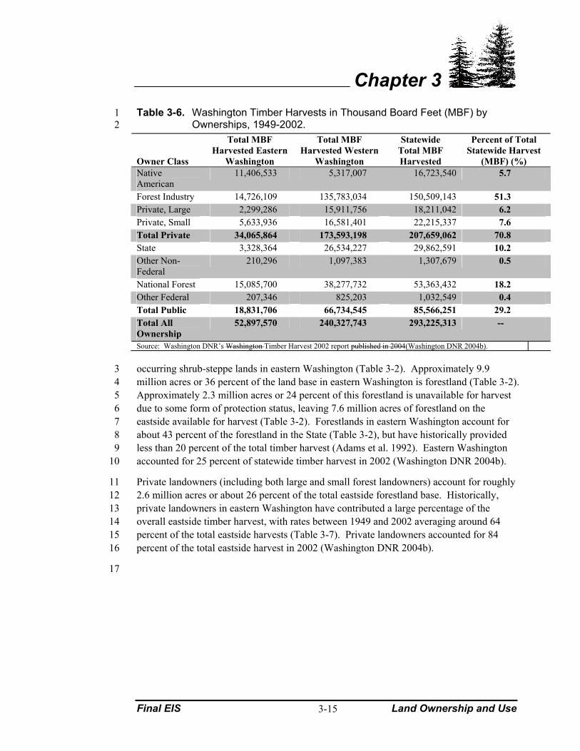
Table 3-6. Washington Timber Harvests in Thousand Board Feet (MBF) by 1 Ownerships, 1949-2002. 2
Owner Class
Total MBF Harvested Eastern
Washington
Total MBF Harvested Western
Washington
Statewide Total MBF Harvested
Percent of Total Statewide Harvest
(MBF) (%) Native American
11,406,533 5,317,007 16,723,540 5.7
Forest Industry 14,726,109 135,783,034 150,509,143 51.3 Private, Large 2,299,286 15,911,756 18,211,042 6.2 Private, Small 5,633,936 16,581,401 22,215,337 7.6 Total Private 34,065,864 173,593,198 207,659,062 70.8 State 3,328,364 26,534,227 29,862,591 10.2 Other Non-Federal
210,296 1,097,383 1,307,679 0.5
National Forest 15,085,700 38,277,732 53,363,432 18.2 Other Federal 207,346 825,203 1,032,549 0.4 Total Public 18,831,706 66,734,545 85,566,251 29.2 Total All Ownership
52,897,570 240,327,743 293,225,313 --
Source: Washington DNR’s Washington Timber Harvest 2002 report published in 2004(Washington DNR 2004b).
occurring shrub-steppe lands in eastern Washington (Table 3-2). Approximately 9.9 3 million acres or 36 percent of the land base in eastern Washington is forestland (Table 3-2). 4 Approximately 2.3 million acres or 24 percent of this forestland is unavailable for harvest 5 due to some form of protection status, leaving 7.6 million acres of forestland on the 6 eastside available for harvest (Table 3-2). Forestlands in eastern Washington account for 7 about 43 percent of the forestland in the State (Table 3-2), but have historically provided 8 less than 20 percent of the total timber harvest (Adams et al. 1992). Eastern Washington 9 accounted for 25 percent of statewide timber harvest in 2002 (Washington DNR 2004b). 10
Private landowners (including both large and small forest landowners) account for roughly 11 2.6 million acres or about 26 percent of the total eastside forestland base. Historically, 12 private landowners in eastern Washington have contributed a large percentage of the 13 overall eastside timber harvest, with rates between 1949 and 2002 averaging around 64 14 percent of the total eastside harvests (Table 3-7). Private landowners accounted for 84 15 percent of the total eastside harvest in 2002 (Washington DNR 2004b). 16
17

Land Ownership and Use Final EIS
Chapter 3
3-16
Table 3-7. Eastern Washington Timber Harvests by Ownerships, 1949-2002. 1
Owner Class
Total Harvest in MBF for
1985-2002
Percent of Total
Harvest for
1985-2002 (%)
Total Harvest in MBF for
1949-1984
Percent of Total Harvest for 1949-1984 (%)
Total Harvest in MBF for
1949-2002
Percent of Total
Harvest for 1949-2002 (%)
Native American
3,793,798 19.7 7,612,735 22.6 11,406,533 21.6
Forest Industry
5,256,791 27.3 9,469,318 28.1 14,726,109 27.8
Private, Large
1,277,501 6.6 1,021,785 3.0 2,299,286 4.4
Private, Small
3,538,796 18.4 2,095,140 6.2 5,633,936 10.7
Total Private
13,866,886 72.1 20,198,978 60.0 34,065,864 64.4
State 1,556,742 8.1 1,771,622 5.3 3,328,364 6.3 Other Non-Federal
61,035 0.3 149,261 0.4 210,296 0.4
National Forest
3,730,678 19.4 11,355,022 33.7 15,085,700 28.5
Other Federal
27,972 0.2 179,374 0.5 207,346, 0.4
Total Public
5,376,427 27.9 13,455,279 40.0 18,831,706 35.6
Total All Ownership
19,243,313 -- 33,654,257 -- 52,897,570 --
Source: Washington DNR’s Washington Timber Harvest 2002 report published in 2004. 2
THE FOLLOWING NEW TEXT REFLECTS PUBLIC COMMENTS ON THE DEIS 3
3.2.4.3 Timber Harvest Rates 4 Rate of harvest information from Washington DNR indicates that for a three-year period 5 from 1988 through 1991, statewide harvests amounted to 3.5 percent of the total available 6 timber supply in Washington State for both partial and even aged harvests combined 7 (Washington DNR 1996). This averages to 1.2 percent per year. This rate slowed slightly 8 between 1991 and 1993 to an average of 1.1 percent per year statewide for both partial and 9 even aged harvests combined (Washington DNR 1997) (Table 3-7a). 10

Final EIS Land Ownership and Use
Chapter 3
3-17
Table 3-7a. Timber Harvest Rates in Washington State, 1988 – 1993. 1 (Rates based on commercial forestland) 2
Time Period
Even Aged Harvest Acres
(Avg/Yr)
Rate of Even Aged Harvest
(Avg/Yr)
Partial Cut Acres Harvested (Avg/Yr)
Rate of Partial Cut Harvest
(Avg/Yr) Western Washington 1988 to 1991 134,970 1.3% 10,653 0.1% 1991 to 1993 109,820 1.0% 12,778 0.1% Eastern Washington 1988 to 1991 48,011 0.5% 43,747 0.5% 1991 to 1993 32,610 0.3% 75,272 0.8% Statewide 1988 to 1991 182,982 0.9% 54,400 0.3% 1991 to 1993 142,430 0.7% 88,050 0.4% Source: Table modified from Washington DNR 1997. Rate of Timber Harvest in Washington State: 1991-1993, Report 2.
3.2.4.4 Timber Supply 3 In 1990, the Washington Legislature commissioned reports from the University of 4 Washington to analyze public and private timber supplies in Washington State. These 5 independent reports, titled Future Prospects for Western Washington’s Timber Supply and 6 Eastern Washington Timber Supply Study Analysis, were produced by the College of 7 Forest Resources in 1992 and 1995, respectively, and described standardized inventories of 8 the timberland base in western and eastern Washington from historic conditions to the 9 early 1990s. 10
Between 1952 and 1990, western Washington’s timberland base had declined by 11 approximately 1 million acres, or about 10 percent of the 1952 level. Approximately half 12 of this decline came from private forestland owners (Adams et al. 1992). Further, the 13 University of Washington reported changes in forestland ownership and cubic feet of 14 growing stock by ownership between 1965 and 1990 (Tables 3-7b and c). These data 15 showed that private forestlands, including both industrial and non-industrial uses, 16 decreased by approximately 4 percent in western Washington between 1965 and 1990. 17 Future projections indicate that by 2089 the acreage of industrial private forestlands will 18 decrease by an estimated 9 percent from initial study conditions and non-industrial private 19 forestlands will decrease by approximately 22 percent (Adams et al. 1992). 20
Land Ownership and Use Final EIS
Chapter 3
3-18
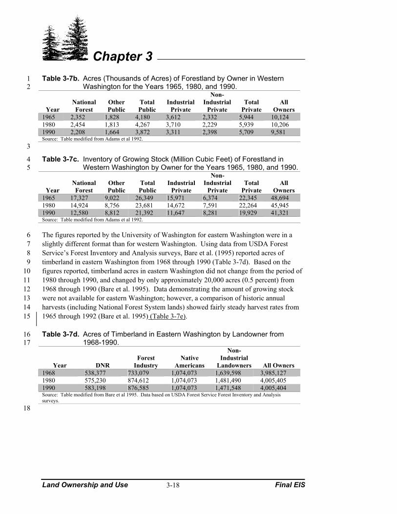
Table 3-7b. Acres (Thousands of Acres) of Forestland by Owner in Western 1 Washington for the Years 1965, 1980, and 1990. 2
Year National Forest
Other Public
Total Public
Industrial Private
Non-Industrial
Private Total
Private All
Owners 1965 2,352 1,828 4,180 3,612 2,332 5,944 10,124 1980 2,454 1,813 4,267 3,710 2,229 5,939 10,206 1990 2,208 1,664 3,872 3,311 2,398 5,709 9,581 Source: Table modified from Adams et al 1992.
3
Table 3-7c. Inventory of Growing Stock (Million Cubic Feet) of Forestland in 4 Western Washington by Owner for the Years 1965, 1980, and 1990. 5
Year National Forest
Other Public
Total Public
Industrial Private
Non-Industrial
Private Total
Private All
Owners 1965 17,327 9,022 26,349 15,971 6,374 22,345 48,694 1980 14,924 8,756 23,681 14,672 7,591 22,264 45,945 1990 12,580 8,812 21,392 11,647 8,281 19,929 41,321 Source: Table modified from Adams et al 1992.
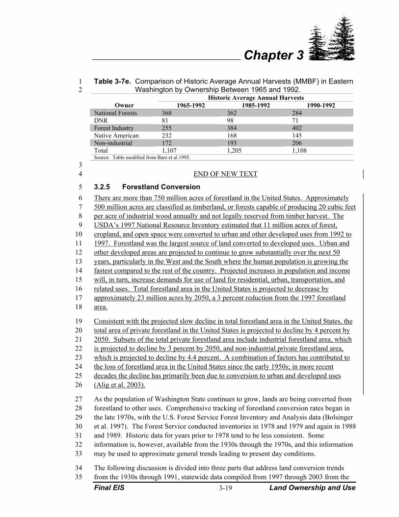
The figures reported by the University of Washington for eastern Washington were in a 6 slightly different format than for western Washington. Using data from USDA Forest 7 Service’s Forest Inventory and Analysis surveys, Bare et al. (1995) reported acres of 8 timberland in eastern Washington from 1968 through 1990 (Table 3-7d). Based on the 9 figures reported, timberland acres in eastern Washington did not change from the period of 10 1980 through 1990, and changed by only approximately 20,000 acres (0.5 percent) from 11 1968 through 1990 (Bare et al. 1995). Data demonstrating the amount of growing stock 12 were not available for eastern Washington; however, a comparison of historic annual 13 harvests (including National Forest System lands) showed fairly steady harvest rates from 14 1965 through 1992 (Bare et al. 1995) (Table 3-7e). 15
Table 3-7d. Acres of Timberland in Eastern Washington by Landowner from 16 1968-1990. 17
Year DNR Forest
Industry Native
Americans
Non-Industrial
Landowners All Owners 1968 538,377 733,079 1,074,073 1,639,598 3,985,127 1980 575,230 874,612 1,074,073 1,481,490 4,005,405 1990 583,198 876,585 1,074,073 1,471,548 4,005,404 Source: Table modified from Bare et al 1995. Data based on USDA Forest Service Forest Inventory and Analysis surveys.
18
Final EIS Land Ownership and Use
Chapter 3
3-19
Table 3-7e. Comparison of Historic Average Annual Harvests (MMBF) in Eastern 1 Washington by Ownership Between 1965 and 1992. 2
Historic Average Annual Harvests Owner 1965-1992 1985-1992 1990-1992
National Forests 368 362 284 DNR 81 98 71 Forest Industry 255 384 402 Native American 232 168 145 Non-industrial 172 193 206 Total 1,107 1,205 1,108 Source: Table modified from Bare et al 1995. 3
END OF NEW TEXT 4
3.2.5 Forestland Conversion 5 There are more than 750 million acres of forestland in the United States. Approximately 6 500 million acres are classified as timberland, or forests capable of producing 20 cubic feet 7 per acre of industrial wood annually and not legally reserved from timber harvest. The 8 USDA’s 1997 National Resource Inventory estimated that 11 million acres of forest, 9 cropland, and open space were converted to urban and other developed uses from 1992 to 10 1997. Forestland was the largest source of land converted to developed uses. Urban and 11 other developed areas are projected to continue to grow substantially over the next 50 12 years, particularly in the West and the South where the human population is growing the 13 fastest compared to the rest of the country. Projected increases in population and income 14 will, in turn, increase demands for use of land for residential, urban, transportation, and 15 related uses. Total forestland area in the United States is projected to decrease by 16 approximately 23 million acres by 2050, a 3 percent reduction from the 1997 forestland 17 area. 18
Consistent with the projected slow decline in total forestland area in the United States, the 19 total area of private forestland in the United States is projected to decline by 4 percent by 20 2050. Subsets of the total private forestland area include industrial forestland area, which 21 is projected to decline by 3 percent by 2050, and non-industrial private forestland area, 22 which is projected to decline by 4.4 percent. A combination of factors has contributed to 23 the loss of forestland area in the United States since the early 1950s; in more recent 24 decades the decline has primarily been due to conversion to urban and developed uses 25 (Alig et al. 2003). 26
As the population of Washington State continues to grow, lands are being converted from 27 forestland to other uses. Comprehensive tracking of forestland conversion rates began in 28 the late 1970s, with the U.S. Forest Service Forest Inventory and Analysis data (Bolsinger 29 et al. 1997). The Forest Service conducted inventories in 1978 and 1979 and again in 1988 30 and 1989. Historic data for years prior to 1978 tend to be less consistent. Some 31 information is, however, available from the 1930s through the 1970s, and this information 32 may be used to approximate general trends leading to present day conditions. 33
The following discussion is divided into three parts that address land conversion trends 34 from the 1930s through 1991, statewide data compiled from 1997 through 2003 from the 35

Land Ownership and Use Final EIS
Chapter 3
3-20
Washington DNR Forest Practices Application Review System, and data compiled for 1 King County since 1982. 2
3.2.5.1 Forestland Conversion from the 1930s to 1991 3 This subsection is divided into three parts: Washington forestlands in the 1930s, forestland 4 conversion from 1945 to 1970, and forestland conversion from 1978 to 1991. 5
Washington Forestlands in the 1930s 6 Data compiled from early forest inventory surveys conducted in the 1930s indicate there 7 were approximately 26.5 million acres of forestlands in Washington State at that time 8 (Table 3-8). These data were collected using a combination of methods including field 9 surveys, analyses of aerial photos, assessment of tax information followed up by field 10 verification, and review of county records and stocking classification of previously logged 11 areas. Approximately 12.5 million acres or 47 percent of forestlands in the State were in 12 private ownership, with 9.1 million acres or 73 percent of private forestlands located in 13 western Washington (Table 3-8). Private forestlands made up 54 percent and 32 percent of 14 forested lands in western and eastern Washington, respectively. 15
The total acres of forestlands available for harvest statewide in all ownerships was 16 approximately 25.2 million acres, of which 15.2 million acres (60 percent) occurred in the 17 western half of the State, and 10.0 million (40 percent) occurred in the eastern half. 18 Federal and State forested reserve lands accounted for 804,848 acres statewide or 3 percent 19 of the total acres of forestland. Of this, 341,178 acres (42 percent) were in western 20 Washington, and 463,670 acres (58 percent) were in eastern Washington (Table 3-8). 21
Table 3-8. Acres of Forestland in Washington State by Ownership in the early 22 1930s. 23
Land Ownership
Western Washington
(Acres)
Eastern Washington
(Acres) Total (Acres) Private 9,055,874 3,432,730 12,488,604 State- Available for harvest 865,346 617,910 1,483,256
State Reserved 11,882 1,680 13,562 County/City 344,882 347,995 692,877 Tribal- Available for harvest 250,648 1,516,490 1,767,138
Federal-Available for harvest 4,652,531 4,075,220 8,727,751
Federal, Other Forestland1/ 356,330 190,685 547,015
Federal Reserved 329,296 461,990 791,286 Total 15,849,289 10,644,700 26,493,989 1/ Includes railroad lands, tribal land grants, and miscellaneous lands. Source: Table modified from Harrington 2003. 24

Final EIS Land Ownership and Use
Chapter 3
3-21
Comparison between these data and estimated forestlands in Washington in 2004 (Tables 1 3-2 and 3-3) suggests that there has been a net loss of approximately 3.5 million acres of 2 forestland since the 1930s, with the majority of this loss (80 percent or 2.8 million acres) 3 occurring in western Washington. These data also suggest that reductions in the amount of 4 privately owned forestland accounted for the majority of this loss. 5
Forestland Conversion from 1945 to 1970 6 As the population of Washington State continues to grow, lands are being converted from 7 forestland to other uses. Comprehensive tracking of forestland conversion rates began in 8 the late 1970s with the U.S. Forest Service Inventory and Analysis data (also known as 9 FIA), which are available in the Forest Service Resource Bulletin PNW-RB-46 (Bolsinger 10 et al. 1997). Data presented in the bulletin estimates that 630,000 acres of commercial 11 forestlands were converted to non-forest uses in Washington over this period, with 12 conversion to urban-industrial, agricultural, and road use (Table 3-9). By 1970 there were 13 an estimated 23.1 million acres of forestland in Washington State, with approximately 4.7 14 million acres in some kind of reserve status (1.6 million acres) or considered not capable of 15 growing commercial timber (3.1 million acres) (Table 3-10). 16
Table 3-9. Conversion of Commercial Forestland in Washington State by 17 Ownership and Land Use, 1945-1970 (In Thousand Acres). 18
Ownership Roads Reservoirs Powerlines Farms1/Urban-
Industrial Miscellaneous Total National Forest 33 10 3 0 0 0 46 Other Public 22 1 33 -182 35 0 73 Forest Industry 50 0 38 13 8 0 109 Farm and Miscellaneous Private
27 9 16 135 214 1 402
Total 132 20 90 130 257 1 630 1/ Farms include lands converted to both agricultural farming and Christmas tree farms. 2/ Minus indicates a gain of forestland. Source: Table modified from Bolsinger 1973.
Table 3-10. Acres of Forestland by Land Class in Washington State, 1970 19 (In Thousand Acres). 20
Land Class Acres of Forestland Commercial Forest 18,401 Commercial Reserved Forest 1,446 Noncommercial Forest1 3,108 Deferred Forest2 143 Total 23,098 1/ This report defined Noncommercial forest to mean forestland that is not capable of growing 20 cubic feet
of industrial wood per year, or is too steep and rocky for harvesting and growing timber crops. 2/ This report defined Deferred forest to mean commercial forestland within National Forests that was being
considered for wilderness designation in 1973. Source: Table modified from Bolsinger 1973.

Land Ownership and Use Final EIS
Chapter 3
3-22
Forestland Conversion from 1978 to 1991 1 Between 1978 and 1991, Bolsinger et al. (1997) estimated that lands available for timber 2 production in Washington outside of the National Forests decreased by 488,000 acres. 3 This figure includes approximately 117,000 net acres of private timberlands that were 4 transferred to the National Forest System, and an additional 92,000 acres (mostly tribal) 5 that were reclassified to reserve status, meaning that they were not available for timber 6 harvest but were still forested lands. Conversions to another use accounted for 7 approximately 279,000 acres. Clearing for rights-of-way for roads, pipelines, and other 8 uses accounted for 155,000 acres or 56 percent of this total (Table 3-11). Most lands 9 converted to rights-of-way were for construction of roads or landings used for logging and 10 forest access, or in the case of other private lands, for connection of private properties, or 11 construction of new or expanding highways or freeways (Bolsinger et al. 1997). 12 Conversions to urban development accounted for 89,000 acres, with the majority of this 13 type of conversion (92 percent) occurring on private, non-industrial forestlands 14 (Table 3-11). 15
Bolsinger et al. (1997) also considered changes over this period in the “primary forest 16 zone,” which they defined as large tracts of forestlands with no more than one development 17 per 640 acres and containing roads that are used primarily for resource extraction and are at 18 least one-quarter mile apart. Uses of this land are primarily restricted to timber production, 19 grazing, watershed, and wildlife protection. Forestlands within this zone were estimated in 20 the 1978 to 1980 inventory to be 7,143,000 acres in western Washington and 6,397,000 21 acres in eastern Washington. Approximately 10 years later, the 1988 to 1991 inventory 22 estimated approximately 6,729,000 acres in this zone in western Washington (a loss of 23 414,000 acres or 6 percent) and 6,384,000 acres in eastern Washington (a loss of 13,000 24 acres or 0.2 percent) (Bolsinger et al. 1997). 25
Adams et al. (1992) found that between 1980 and 1990 all ownership groups had a net loss 26 of forest acres except for non-industrial private landowners, which reported a net gain of 27 169,000 acres. However, it was not clear if this gain was from lands converted back into 28 forest production or if it was simply land purchases. Adams et al. (1992) attributed 90 29 percent of the total acreage of forestland conversions to non-forest uses between 1980 and 30
Table 3-11. Changes in Forestland Area by Ownership and Land Use in 31 Washington State from 1978-1991. 32
Other Public1/ Forest Industry2/ Other Private3/ Total Rights-of-way -12,000 -95,000 -48,000 -155,000 Urban 0 -7,000 -82,000 -89,000 Agriculture4/ 0 0 -53,000 -53,000 Reclaimed Forest 0 6,000 12,000 18,000 Total -12,000 -96,000 -171,000 -279,000 1/ Lands administered by public agencies other than the USDA Forest Service. 2/ Lands owned by companies that grow timber for industrial uses. 3/ Private lands not owned by the forest industry, but including tribal lands, farmer-owned lands, and miscellaneous other private
lands. 4/ Agricultural lands, including Christmas tree farms, converted to forestland. Source: Bolsinger et al. 1997

Final EIS Land Ownership and Use
Chapter 3
3-23
1990 to development such as urban uses (130,000 acres) or rights-of-way development 1 (50,000 acres). 2
3.2.5.2 Washington Department of Natural Resources Data 3 Four classes of forest practices have been established based on the potential of planned 4 activities to adversely impact public resources. Forest practices are classed as I, II, III, or 5 IV, with Class I having no potential of damaging public resources and Class IV having the 6 greatest potential. Class IV forest practices are further distinguished as Class IV-Special or 7 Class IV-General by rule of the Washington Forest Practices Board. Class IV-Special 8 forest practices are those that have been determined to have potential for a substantial 9 impact on the environment. Class IV-General are forest practices on lands platted after 10 January 1, 1960, or on lands being converted to another use, or that will not be reforested 11 because of a likelihood of future conversion to urban development. 12
Conversion information available from Washington DNR’s Forest Practices Application 13 Review System database indicate that 53,821 acres of forestland were converted to other 14 uses between 1997 and 2003, with an average of 7,687 acres per year statewide (Table 15 3-12). These data are based on Class IV-General forest practices applications approved by 16 the Washington DNR. Some margin of error is expected due to the fact that not all 17 landowners report conversions of lands that were harvested under a different application 18 class, and not all landowners who apply to convert their lands actually follow through with 19 the land conversion. 20
Transfer of Authority for Class IV – General Applications 21 While the Forest Practices Board is the entity responsible for establishing forest practices 22 standards that serve as the basis for the Forest Practices Regulatory Program, and the 23 Washington DNR is the agency charged with managing Program implementation, some 24 local governments have authority over Class IV-General forest practices within their 25 jurisdiction. In accordance with the Revised Code of Washington (RCW) (RCW Chapter 26 76.09.240), the Washington DNR is in the process of working with local governments to 27 transfer jurisdiction of Class IV-General forest practices. 28
Table 3-12. Acres of Forestlands Converted to Other Uses by Year. 29
Year Total Acres Western
Washington Total Acres Eastern
Washington Total Acres Statewide
1997 4,059.2 3,095.6 7,154.8 1998 3,748.1 3,675.8 7,423.9 1999 3,320.7 3,351.1 6,702.2 2000 3,143.8 1,863.8 5,007.6 2001 7,374.2 1,258.6 8,632.8 2002 2,223.6 3,794.9 6,018.5 2003 10,083.5 2,797.3 12,880.8 Total 33,953 19,837 53,821
Source: Washington DNR FPARS Data Base, January 2004.

Land Ownership and Use Final EIS
Chapter 3
3-24
Each city and county in the State is required to adopt ordinances by December 31, 2005 to 1 regulate Class IV-General forest practices. The city or county’s ordinances or regulations 2 must meet or exceed the standards set forth in the current Washington Forest Practices 3 Rules. Washington DNR, in consultation with Washington Department of Ecology 4 (Ecology), may approve or disapprove the regulations in whole or in part (RCW Chapter 5 76.09.240(3). To date, Washington DNR has transferred authority to regulate Class IV-6 General forest practices to four counties: Thurston, King, Spokane, and Clark Counties. 7 Generally, forest practices inside designated urban growth areas are likely to be associated 8 with future conversion to another land use, while forest practices outside urban growth 9 areas are not. In high population growth areas, development pressures may result in more 10 Class IV-General conversions outside the urban growth area than in areas with lower 11 growth rates. 12
3.2.5.3 King County Data 13 King County, the most populated county in the State, has kept relatively complete data on 14 Class IV-General conversions of forestland since about 1982. The average conversion rate 15 from 1982 to 1987 was about 675 acres per year, which grew in the late 1980s to an 16 average of 1,500 acres per year (Personal Communication, Chandler Felt, King County 17 Department of Development and Environmental Studies, February 19, 2004). Conversion 18 rates in King County slowed to an average of about 600 acres per year after the adoption of 19 the 1990 Growth Management Act and because of economic slowdowns also experienced 20 at that time. In 1998, another short-lived conversion boom occurred (1,500 acres), after 21 which the average dropped back down to 490 acres per year (Personal Communication, 22 Chandler Felt, King County Department of Development and Environmental Studies, 23 February 19, 2004) (King County 2000) (Table 3-13). Additionally, in 1994, King County 24 designated Forest Production Districts under the Growth Management Act, which 25 established zoning restrictions and other regulations designed to encourage timber 26 production in those districts. 27
Table 3-13. Forest Practices Applications and Acres of Converted Forestland in 28 King County, 1990 through 1998. 29
Inside Forest Production Areas Outside Forest Production Areas
Year
Total Acres
Converted Forested Acres
Converted
Number of Conversion
Applications Forested Acres
Converted
Number of Conversion
Applications 1990 728 1 5 727 56 1991 426 71 12 355 17 1992 445 7 1 438 27 1993 1,131 13 4 1,118 96 1994 306 0 0 306 32 1995 674 0 0 674 41 1996 754 4 1 750 55 1997 541 58 3 483 34 1998 1,483 145 5 1,338 27 Total 6,488 299 31 6,189 385 Source: King County 2000 Annual Growth Report; Personal Communication, Chandler Felt, King County Department of Development
and Environmental Services, February 19, 2004.
30

Final EIS Air Quality
Chapter 3
3-25
3.3 AIR QUALITY 1 Air quality is regulated by the Federal Clean Air Act, which requires the Environmental 2 Protection Agency (EPA) to set national ambient air quality standards for pollutants 3 considered harmful to public health and the environment. “Ambient air” refers to that 4 portion of the atmosphere, external to buildings, to which the general public has access. 5 An air quality standard establishes values for maximum acceptable concentration, exposure 6 time, and frequency of occurrence of one or more air contaminants in the ambient air. 7 Ambient air quality standards have been set for six principal pollutants: carbon monoxide, 8 nitrogen dioxide, ozone, lead, particulate matter, and sulfur dioxide. The State of 9 Washington has an approved State Implementation Plan, which regulates, among other 10 pollutants and emissions from prescribed burning (Washington Department of Ecology 11 1999a). The State Implementation Plan also addresses particulate mater (including 12 “PM10”), visibility, and smoke management. 13
Prescribed burning on forestland is regulated by Washington DNR’s Resource Protection 14 Division, which requires a permit for burning. Washington DNR’s federally mandated 15 Smoke Management Plan (Washington Administrative Code [WAC] 173-425-120; State 16 adopted October 18, 1990, EPA effective January 15, 1993) ensures that forest 17 management-related burning activities comply with the Clean Air Act and provides 18 regulatory direction, operating procedures, and information regarding the management of 19 smoke and fuels on the forestlands of Washington (Washington DNR 1993). The plan 20 coordinates and facilitates the statewide regulation of prescribed burning on Federal and 21 non-Federal forestlands and participating tribal lands. Washington DNR follows the 22 guidelines set forth in this plan when issuing and regulating burning permits for open fire 23 when such fires are for the following: 24
1. Abating a forest fire hazard 25 2. Preventing a fire hazard in a forested area 26 3. Instructing public officials in methods of forest fire fighting 27 4. Any silvicultural operation to improve the forestlands of the State 28
In particular, three potential sources of particulate air pollution associated with forest 29 management activities are slash burning, wildfire, and road use. Managers of non-Federal 30 forestlands in Washington typically use slash burning as part of their site preparation 31 activities, usually by concentrating slash in piles and burning the piles (slash concentrated 32 burning) rather than by broadcast burning, as was more common in the past. Broadcast 33 burning is the practice of burning logging slash scattered throughout a recently harvested 34 unit to prepare the site for planting and/or to reduce dangerous fuel loads. Burning is 35 usually done in the spring or fall under wetter conditions when fewer particulates are 36 emitted than would be the case if the same fuels burned in a wildfire. Particulate emissions 37 from wildfires are, on average, three to four times higher than from prescribed burning 38 (Washington DNR 1996). 39
The use of logging roads during dry weather conditions generates air-borne dust. Air-40 borne dust is regulated through road maintenance standards of the Washington Forest 41 Practices Board (WAC 222-24) and safety standards of the Washington Department of 42

Air Quality Final EIS
Chapter 3
3-26
Labor and Industries (WAC 296-54). The amount of air-borne dust is a function of road 1 use and surfacing material. Gravel can reduce dust on dirt roads (Washington Department 2 of Ecology 2001) as can water and chemical dust suppressants. In general, the adverse 3 effects of air-borne dust are localized and short term (Washington DNR 1996). 4
The main sources of air pollution in western Washington include motor vehicles (55 5 percent), industrial (13 percent), and wood stoves (9 percent). Approximately 4 percent is 6 generated from outdoor burning, a portion of which comes from forest management 7 activities (Washington Department of Ecology 2003). Air quality in Washington is 8 generally good or moderate, although some areas do not meet Federal standards on some 9 days. Air quality has improved greatly since 1987, when Washington violated air quality 10 standards on 150 days. This figure dropped to 7 percent in 1999 (Washington Department 11 of Ecology 2003). 12
One of the ecological benefits of forested lands is the enhancement of air quality. Plants 13 enhance air quality by emitting oxygen and consuming carbon dioxide, the gas most 14 associated with global warming. In addition, trees retard the spread of air-borne 15 particulates by trapping the material on their leaf surfaces and by slowing the wind speed 16 to the point that particulates cannot remain suspended. Timber harvesting temporarily 17 removes the air quality benefits provided by trees (Washington DNR 1996). 18
19
Final EIS Geology, Soils, and Erosional Processes
Chapter 3
3-27
3.4 GEOLOGY, SOILS, AND EROSIONAL PROCESSES 1
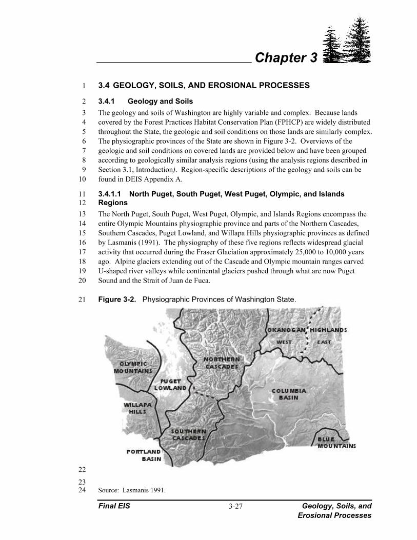
3.4.1 Geology and Soils 2 The geology and soils of Washington are highly variable and complex. Because lands 3 covered by the Forest Practices Habitat Conservation Plan (FPHCP) are widely distributed 4 throughout the State, the geologic and soil conditions on those lands are similarly complex. 5 The physiographic provinces of the State are shown in Figure 3-2. Overviews of the 6 geologic and soil conditions on covered lands are provided below and have been grouped 7 according to geologically similar analysis regions (using the analysis regions described in 8 Section 3.1, Introduction). Region-specific descriptions of the geology and soils can be 9 found in DEIS Appendix A. 10
3.4.1.1 North Puget, South Puget, West Puget, Olympic, and Islands 11 Regions 12 The North Puget, South Puget, West Puget, Olympic, and Islands Regions encompass the 13 entire Olympic Mountains physiographic province and parts of the Northern Cascades, 14 Southern Cascades, Puget Lowland, and Willapa Hills physiographic provinces as defined 15 by Lasmanis (1991). The physiography of these five regions reflects widespread glacial 16 activity that occurred during the Fraser Glaciation approximately 25,000 to 10,000 years 17 ago. Alpine glaciers extending out of the Cascade and Olympic mountain ranges carved 18 U-shaped river valleys while continental glaciers pushed through what are now Puget 19 Sound and the Strait of Juan de Fuca. 20
Figure 3-2. Physiographic Provinces of Washington State. 21
22
23 Source: Lasmanis 1991. 24
Geology, Soils, and Final EIS
Erosional Processes
Chapter 3
3-28
In addition to shaping the topography of the regions, glaciers blanketed large areas with 1 till, outwash, and lake sediments. These glacial deposits served as parent materials on 2 which many of the regions’ soils have developed. Glaciers left behind landforms that 3 range from nearly flat glacial plains in the Puget Lowland to very long, steep mountain 4 slopes in the Northern and Southern Cascades and Olympic Mountains physiographic 5 provinces. 6
While Quaternary glacial deposits dominate areas that lie within the Puget Lowland 7 physiographic province, other areas contain highly diverse rock types. The most common 8 geologic units in the Northern Cascades and Olympic Mountains include sedimentary and 9 volcanic rocks from the Lower Tertiary Period and Mesozoic Era and intrusive igneous 10 rocks from the Tertiary Period. 11
The relatively short time since deglaciation has limited the degree of soil development in 12 many parts of these regions. The glacial deposits and other parent materials remaining 13 after deglaciation have not undergone the higher levels of physical and chemical 14 weathering and related soil formation found in non-glaciated areas of the State. Soils 15 developed on glaciated terrain tend to have much lower levels of organic matter in their 16 surface horizons and less horizon development than older, more heavily weathered soils in 17 other parts of Washington. Soils developed from glacial parent materials are common at 18 low elevations, as are alluvial soils along major rivers and streams. The primary types of 19 glacial parent materials, in order of their relative coverage, are glacial till, glacial outwash, 20 and glacial lake sediments. At moderate to high elevations, soils are more commonly 21 formed from a mixture of colluvial bedrock materials, glacial drift deposits, and volcanic 22 ash (Washington DNR 1996). 23
3.4.1.2 Southwest and Lower Columbia Regions 24 The Southwest and Lower Columbia Regions encompass the Willapa Hills and Portland 25 Basin physiographic provinces and parts of the Olympic Mountains, Puget Lowland, and 26 Southern Cascades provinces as defined by Lasmanis (1991). Unlike analysis regions to 27 the north, many parts of the Southwest and Lower Columbia Regions were never glaciated. 28 As a result, highly weathered rocks that are relatively easily erodible remain widespread, 29 particularly in the Southwest Region and the western portions of the Lower Columbia 30 Region. Erosion of these rocks has produced hills and ridges that are rounded with short, 31 steep slopes and low gradient stream channels. 32
The eastern part of the Lower Columbia Region includes portions of the Southern 33 Cascades physiographic province that was subject to alpine glaciation during the 34 Pleistocene Epoch. This area is similar to the glaciated northern regions where broad, U-35 shaped valleys and long, steep slopes are common. Typical geologic units in the 36 Southwest and Lower Columbia Regions are Quaternary Period sediments (including 37 alluvial and coastal deposits), Tertiary Period sedimentary rocks, and Lower Tertiary 38 volcanic rocks. 39
Due to the limited influence of glacial activity in these regions, soils tend to be older, 40 deeper, finer in texture, and have a higher nutrient status relative to soils in the northern 41
Final EIS Geology, Soils, and Erosional Processes
Chapter 3
3-29
analysis regions described earlier. Due to these soil characteristics and the generally 1 favorable climatic conditions, the average potential productivity of covered lands in the 2 Southwest and Lower Columbia Regions tends to be higher than in other regions. 3
Most non-alluvial soils have formed on parent materials derived from the underlying 4 bedrock. Topography strongly influences the character and behavior of these soils. On 5 steeper slopes, soils tend to be shallower, have higher gravel contents and lower potential 6 productivities relative to soils on more gentle terrain. This is primarily due to the increased 7 potential for surface erosion and mass wasting on steeper slopes (Washington DNR 1996). 8
3.4.1.3 Middle and Upper Columbia (Downstream of Grand Coulee Dam) 9 Regions 10
The Middle and Upper Columbia (Downstream of Grand Coulee Dam) Regions include 11 portions of the Southern Cascades, Northern Cascades, and Columbia Basin physiographic 12 provinces as defined by Lasmanis (1991). These Regions largely consist of eastward 13 trending river valleys that are deeply dissected and separated by sharp ridge crests. 14 Volcanic rocks of the Columbia River Basalt Group and younger Quaternary volcanics, 15 including andesite and basalt flows, dominate the geology in the Middle Columbia Region. 16 Deposits of alpine glacial sediments are also scattered throughout the Region at higher 17 elevations. 18
Further north, the Upper Columbia Region (downstream of Grand Coulee Dam) lies within 19 the rugged Northern Cascades where the influence of glaciation is more apparent. All but 20 the highest peaks in the Region have been heavily glaciated and the valleys of Columbia 21 River tributaries have relatively flat bottoms and steep walls. Dominant geologic units 22 include Lower Tertiary Period and Mesozoic Era sedimentary and intrusive igneous rocks. 23 Both Regions transition into the Columbia Basin physiographic province near their eastern 24 boundaries where topographic relief decreases. Non-glacial Quaternary Period sediments 25 and rocks of the Columbia River Basalt Group dominate the geology of the Columbia 26 Basin. 27
Climatic differences between the analysis regions of western Washington described earlier 28 and those of eastern Washington have produced substantial differences in soils. The 29 Middle and Upper Columbia (downstream of Grand Coulee Dam) Regions lie in the rain 30 shadow of the Cascades and the low precipitation levels limit soil profile development and 31 forest productivity (Washington DNR 1996). 32
Areas closer to the eastern edges of the analysis regions have the lowest levels of soil 33 development and potential productivity because they have the lowest average annual 34 precipitation. Areas in the western portions of the analysis regions tend to have greater soil 35 development and higher productivity than in the eastern portions because of their higher 36 average annual precipitation. However, productivity is limited at higher elevations due to 37 the shorter growing season (Washington DNR 1996). 38

Geology, Soils, and Final EIS
Erosional Processes
Chapter 3
3-30
3.4.1.4 Upper Columbia (Upstream of Grand Coulee Dam) Region 1 The Upper Columbia (upstream of Grand Coulee Dam) Region roughly coincides with the 2 Okanogan Highlands physiographic province as defined by Lasmanis (1991). The Region 3 is characterized by rounded mountains and deep, narrow valleys. The eastern half of the 4 Region contains the oldest rocks in the State. Dominant geologic units include Paleozoic 5 Era and Precambrian sedimentary rocks and Mesozoic Era intrusive igneous rocks. The 6 western half of the Region was formed by offshore deposition of sediments and volcanic 7 rocks west of the continental margin during the Lower Tertiary Period, Glacial ice covered 8 the Region during the Quaternary Period, reshaping the landscape and forming lakes in the 9 Columbia and Pend Oreille River valleys. 10
Soil productivity in the Upper Columbia (upstream of Grand Coulee Dam) Region is tied 11 closely to annual precipitation. The areas with higher annual precipitation generally have 12 deeper, more productive soils than drier areas. 13
3.4.1.5 Snake River Region 14 The Snake River Region includes the entire Blue Mountains physiographic province and 15 part of the Columbia Basin province as defined by Lasmanis (1991). The Blue Mountains 16 are characterized by a broad geologic uplift reaching elevations of more than 6,000 feet 17 above sea level. Rocks of the Columbia River Basalt Group dominate the Region’s 18 geology. Quaternary sediments derived largely from glacial outburst floods and eolian 19 deposits are common at lower elevations in the Columbia Basin province. 20
Many soils in the Blue Mountains have developed from wind-deposited sediments known 21 as loess. These soils tend to be fine-textured and moderately productive. Soil productivity 22 is somewhat influenced by topography, with soils on steeper slopes tending to be more 23 shallow and less productive than soils on gentler terrain. 24
3.4.2 Erosion 25 Erosion is the detachment and movement of soil particles either individually, in small 26 aggregates, or in large masses (Brooks et al. 1991). The two dominant processes of 27 erosion on forestlands are surface erosion and mass wasting. Surface erosion is the 28 detachment and subsequent removal of soil particles and small aggregates from land 29 surfaces by wind or water. Mass wasting includes erosion in which cohesive masses of 30 soil are displaced. Debris avalanches, debris flows, and debris torrents are mass wasting 31 processes that transport material rapidly. Debris avalanches are shallow, rapid landslides 32 on steep hillslopes (Chatwin et al. 1991). If enough water is present, debris avalanches 33 become debris flows that rapidly transport soil, rocks, and organic material directly to the 34 valley floor and occasionally to stream channels (Chatwin et al. 1991). Where debris 35 avalanches and debris flows reach steep stream channels during peak flow periods, debris 36 torrents occur, involving the rapid movement of large volumes of water-charged soil, rock, 37 and debris (Chatwin et al. 1991). Rates of movement are very high (feet/second) and 38 damage can be extensive. Another class of mass wasting processes includes deep-seated 39 landslides that, unlike debris avalanches, debris flows, and debris torrents, tend to have 40 failure planes greater than 10 feet below the ground surface. Also, deep-seated landslides 41
Final EIS Geology, Soils, and Erosional Processes
Chapter 3
3-31
generally have slower rates of movement (i.e., feet/year to feet/day) although rapid 1 movement (i.e., feet/minute to feet/second) is possible. Under natural conditions, mass 2 wasting is the more common form of erosion on forestlands in the Pacific Northwest, 3 particularly in steep terrain (Sidle et al. 1985). 4
Dam break floods occur when water impounded behind material such as woody debris 5 and/or coarse sediment breaks through the “dam” releasing a large discharge of water 6 through the channel. These events can release sediment, scour and temporarily change 7 channel morphology. 8
The relative importance of different erosion processes on covered lands within the various 9 analysis regions is summarized below. This information largely reflects findings of the 10 approximately 60 watershed analyses completed in Washington since 1993. 11
3.4.2.1 Erosion Processes on Covered Lands 12 North Puget, South Puget, West Puget, Olympic, and Islands Regions 13 Mass wasting is the dominant form of erosion in these glaciated regions (Washington DNR 14 1993, 1994a, 1995a, and 1996b). Steep, mountainous terrain combined with high 15 precipitation levels produces high rates of mass wasting. Debris avalanches, debris flows, 16 debris torrents, and dam-break floods are common in most regions (the exception being the 17 Islands Region) and are most often associated with large magnitude rain or rain-on-snow 18 events that occur during the fall and winter months (Washington DNR 1998a). Debris 19 torrents and dam-break floods are usually associated with high-gradient, confined 20 headwater streams and may translate downstream for several miles (Coho and Burgess 21 1991). Deep-seated landslides are fairly common and occur most frequently in areas of 22 structurally weak bedrock or glacial lake deposits (Washington DNR 1998b). Even though 23 many soils are shallow, high organic matter contents generally produce high infiltration 24 capacities, so surface erosion is limited to disturbed and/or compacted soils. 25
Southwest and Lower Columbia Regions 26 The Southwest and Lower Columbia Regions are similar to those described above in that 27 mass wasting is the dominant form of erosion (Washington DNR 1994b, 1995b, and 28 1998c). While topographic relief is low relative to the more heavily glaciated regions to 29 the north, steep slopes and high precipitation levels produce high rates of mass wasting. 30 Debris avalanches and debris flows are very common; however, short slope lengths and 31 low channel gradients make debris torrents and dam-break floods less common. High 32 frequencies of deep-seated landslides occur in certain geologic units (Washington DNR 33 1998c). Soils generally have high infiltration capacities, so surface erosion is limited to 34 disturbed and compacted soils. 35
Middle and Upper Columbia and Snake River Regions 36 The lower annual precipitation and more moderate topography east of the Cascade crest 37 generally results in a lower incidence of mass wasting than on the westside; however, 38 debris avalanches, debris flows, debris torrents, and dam-break floods all occur to varying 39 degrees. On the east slopes of the Cascade Range and in the Columbia River Gorge, these 40 mass wasting processes are usually driven by rain or rain-on-snow events during the fall 41

Geology, Soils, and Final EIS
Erosional Processes
Chapter 3
3-32
and winter months (Washington DNR 1998d, 1998e). In the Okanogan Highlands of 1 northeastern Washington, rapid spring snowmelt and spring thunderstorms typically 2 initiate mass wasting (Personal Communication, Jack Powell, Washington DNR, March 3 2004). Deep-seated landslides are most often associated with interbeds of sediments 4 between basalt flows of the Columbia River Basalt Group throughout eastern Washington 5 and glacial lake sediments in the northeastern part of the State (Personal Communication, 6 Jack Powell, Washington DNR, March 2004). Many soils have low organic matter 7 contents, making infiltration capacities low relative to soils in western Washington. Also, 8 relatively low annual precipitation makes vegetation recovery slower than in western 9 Washington. Relatively low infiltration capacities and longer revegetation periods make 10 surface erosion fairly common, particularly in areas with disturbed and compacted soils 11 (Washington DNR 1995c, 1997d). 12
3.4.2.2 Forest Practices Effects on Erosion and Sedimentation 13 Forest practices such as timber harvesting and road construction have the potential to 14 accelerate the rate of erosion by disturbing soils, reducing infiltration and increasing 15 surface runoff (Swanson et al. 1987). Accelerated rates of erosion can lead to increased 16 sediment delivery to channel networks where it can negatively affect aquatic resources. 17 Increased sediment supply to streams can reduce the quantity and quality of habitat for 18 aquatic organisms such as fish, amphibians, and macroinvertebrates (Bisson et al. 1987). 19 The following discussion provides an overview of various forest practices activities and 20 their effects on erosion, sediment delivery, and aquatic resources. 21
Road-Related Surface Erosion 22 Road-related surface erosion is a function of the intensity of road use; road surfacing 23 materials, construction, and maintenance types; the intensity and amount of precipitation; 24 and other factors (Reid and Dunne 1984; Megahan and Kidd 1972). Road construction, 25 use, maintenance, abandonment, and drainage all play important roles in the production 26 and delivery of sediment to streams, ponds, lakes, wetlands, and marine areas. Surface 27 erosion from roads tends to be a chronic source of fine sediment to the drainage network. 28 Chronic sources of fine sediment can adversely impact the physical habitat of the aquatic 29 system and certain life stages of fish, aquatic insects and amphibians, and also degrade 30 water quality. 31
Road density can be used to help understand the potential for impacts from road surface 32 erosion, drainage, and sediment delivery to streams. As mentioned earlier, many factors 33 affect the degree of impact to aquatic resources from roads, and there can be a greater 34 possibility of adverse impacts as road density in a watershed increases. However, the body 35 of research on this subject indicates the relationship between the degree of impacts to 36 aquatic resources and road density is not simple and linear. Nonetheless, road density may 37 be used as an indicator variable. Road densities were estimated within the FPHCP covered 38 lands for the 12 analysis regions. DEIS Appendix D, Table D.1 shows the average road 39 density by region and by WRIA, as well as the overall average road density for covered 40 lands. Estimated average road density in the 12 regions ranged from 2.5 to 4.9 miles of 41 road per square mile of covered lands with an overall average road density of 3.4 miles per 42

Final EIS Geology, Soils, and Erosional Processes
Chapter 3
3-33
square mile. A description of the process to estimate road density is included with DEIS 1 Appendix D, Table D.1. 2
Studies of the hydrologic impacts of forest roads indicate that the dominant source of road 3 runoff is intercepted subsurface storm water flow, where permeable soil intercepts 4 relatively impermeable bedrock (LaMarche and Lettenmaier 2001; Bowling and 5 Lettenmaier 2001). Sediment delivery from road surfaces to streams is dependent on 6 connectivity between streams and road surfaces. Adequate road construction, 7 maintenance, and abandonment would accommodate most storm events, minimize road 8 erosion by traffic and precipitation events, and minimize delivery of road surface sediment 9 to the stream network. 10
Currently, Road Maintenance and Abandonment Plans (RMAPs) are required for large 11 landowners subject to the Washington Forest Practices Rules. The total road mileage 12 accounted for under RMAPs as of March 2004 is approximately 40,000 miles. 13 Approximately 11,000 miles of those are in eastern Washington, and 29,000 miles are in 14 western Washington. Under current rules, large landowners must have all of their roads 15 under approved RMAPs by 2006. Small landowners, other than 20-acre exempt 16 landowners, have the option to submit an RMAP checklist or RMAP when they submit a 17 forest practices application. The small landowner RMAP checklist submitted with the 18 forest practices application must cover the haul roads being used under the forest practices 19 application and does not have to cover other roads the landowners may own. The 20-acre 20 exempt landowner does not have to submit an RMAP or RMAP checklist. Correction of 21 all road problems for large landowners must occur by 2016. Correction of road problems 22 for small landowners generally occurs at the time a landowner files a forest practices 23 application that includes a road-related problem, and the Washington Forest Practices 24 Rules require them to maintain roads used for timber hauling in a condition that prevents 25 damage to public resources. Quantification of the risks of road-related sediment 26 production and delivery to streams is not completed. However, an adaptive management 27 research and effectiveness monitoring study is under development to evaluate road 28 sedimentation under the current Washington Forest Practices Rules. 29
Road-Related Mass Wasting 30 Debris avalanches, debris flows, and debris torrents are episodic sources of fine and coarse 31 sediment to the aquatic system. These erosion processes can be greatly accelerated by road 32 management practices. Many studies have shown that on a unit area basis, roads have the 33 greatest effect on mass wasting of all activities on forestlands (Sidle et al. 1985). 34 However, some research suggests that harvest-related mass wasting occurs with 35 approximately the same frequency as road-related landslides (Montgomery et al. 1998). 36 Road location, drainage, design, construction, and maintenance are all-important factors in 37 effective road design, but can be contributing factors to road-related failure. New road 38 construction and engineering design has reduced road-related mass wasting relative to 39 roads constructed more than 15 to 20 years ago (Toth 1991; Robison et al. 1999). 40

Geology, Soils, and Final EIS
Erosional Processes
Chapter 3
3-34
Orphan Roads 1 Orphan roads are roads constructed prior to 1974 that have not been used for forest 2 practices since that time (WAC 222-24-052*(4)). Such roads are typically not maintained, 3 and many were constructed without a requirement to consider public resource and channel 4 impacts. The mileage of orphan roads in Washington is unknown; however, the associated 5 hazards have been identified. The concern with orphan roads is the lack of knowledge 6 about their location and potential for failure and initiation of debris avalanches, debris 7 flows, and debris torrents. Large landowners are inventorying and assessing their orphan 8 roads and showing the orphan roads’ locations in their RMAPs. The goal of the orphan 9 roads inventory is to locate the roads and assess the condition of the roads to determine 10 what work needs to be done to protect resources from orphan road failures and how the 11 cost of that work might be funded. 12
Harvest-Related Surface Erosion 13 Surface erosion is dependent on many variables. The primary variables are slope, soil 14 texture, and vegetation cover (Benda et al. 1998). 15
Harvest activities such as ground skidding or cable yarding can cause some degree of soil 16 disturbance. Typically, ground-based systems compact and disturb more soils than non-17 ground-based harvest systems (Graham et al. 1991). The harvest systems most likely to 18 cause greater levels of disturbance (from greatest to lowest) are ground-based systems, 19 cable yarding, and aerial systems (Beschta and Boyle et al. 1995). Clearcuts tend to create 20 the greatest area of soil disturbance (Hermann 1978); however, disturbance from felling, 21 yarding, and skid trails in partial cuts can also cause ground disturbance and compaction. 22 Cromack et al. (1978) found levels of soil disturbance in clearcut and partial cut areas to be 23 comparable because of the need for equivalent access through a harvest unit. 24
Streamside buffers can substantially reduce fine sediment that is transported overland 25 (Rashin et al. 1999). The capacity of riparian buffers to control sediment inputs from 26 surface erosion depends on several site characteristics including the presence of vegetation 27 or organic litter, slope, soil type, and drainage characteristics. Additionally, the filtering 28 capacity is affected by timber harvest activities within the buffer. Although soil 29 disturbance generally increases the sediment delivery potential, the addition of obstructions 30 on the forest floor from tree limbs and boles (limb-free trunks) associated with partial 31 logging can offset diminished filtration (Burroughs and King 1989; Benoit 1979). These 32 factors influence the ability of buffers to trap sediment by controlling the infiltration rate of 33 water and the velocity of overland flow. 34
Riparian protection measures should also include practices for minimizing sediment 35 contributions from outside the riparian area. Timber harvest activities can disturb the 36 upper soil layers, exposing the subsoil to erosion. A study of sediment delivery from 37 timber harvest was conducted by Rashin et al. (1999) between 1992 and 1995, prior to the 38 current Washington Forest Practices Rules. This study evaluated specific harvest practices 39 on State and private lands across Washington. Harvest sites were evaluated for soil 40 exposed and sediment delivered, and was categorized by a number of parameters, including 41 harvest method and distance from streams. They found that in areas where there were no 42

Final EIS Geology, Soils, and Erosional Processes
Chapter 3
3-35
buffers, best management practices (BMPs) for timber harvest were not effective in 1 preventing soil disturbance or preventing sediment from reaching streams. They also 2 found that no-harvest buffers at least 30 feet wide were effective in filtering sediment, 3 although they caution use of these results because of low precipitation and storm events 4 during the study period. 5
Harvest-Related Mass Wasting 6 Debris Avalanches and Debris Flows 7 Debris avalanches and debris flows are the most common types of landslides in steep 8 forestlands. Still, only 2 percent of the landscape is affected at any given time (Ketcheson 9 and Froelich 1978; Ice 1985). Debris avalanches and debris flows are typically initiated by 10 high magnitude rain or rain-on-snow events during the fall and winter months (Swanson et 11 al. 1987). Sidle et al. (1985) summarized several studies (Swanston 1970, 1974; 12 O’Loughlin 1974; Ziemer and Swanston 1977; Burroughs and Thomas 1977; Gray and 13 Megahan 1981; Ziemer 1981) indicating that slope stability depends partly on 14 reinforcement from tree roots, especially when soils are partly or completely saturated. 15 Clearcut timber harvesting on unstable slopes or landforms decreases rooting strength, 16 increasing the potential frequency and magnitude of debris avalanches and debris flows 17 (Ziemer and Swanston 1977; Wu and McKinnell III 1978). 18
Debris Torrents 19 Debris avalanches and debris flows can turn into debris torrents. Debris torrents usually 20 transport more material than the initiating event, due to scouring action on the slope or in 21 the channel. Debris torrents stop moving when the channel gradient decreases 22 substantially or when the torrent encounters a sharp bend in the channel. Debris torrents 23 contain substantial amounts of wood and can travel varying distances, which can result in 24 variable degrees of impact depending upon channel gradient, confinement, layout of the 25 channel network, and other characteristics (Fannin and Rollerson 1993). Debris torrents 26 can have long-lasting effects on stream channels. The channel location and cross-section 27 can be radically altered in such a way that normal flows and normal peak flows cannot 28 reconfigure the channel easily (Lamberti et al. 1991). This is important because even 29 though mass wasting in general may affect only 1 percent of a watershed, debris torrents 30 can affect up to 10 percent of the stream system because of their mobility (Swanson et al. 31 1987). These channel alterations from debris torrents, however, are not always negative. 32 For example, Benda et al. (2003) found that channel morphology and habitat complexity 33 (e.g., pool density, substrate texture, and channel widths) increased in proximity to low-34 order (See Glossary) tributary confluences prone to debris flows. In addition to having 35 impacts on the stream channel, debris torrents can also affect riparian buffer functions and 36 streamside forests when bank scour is so great that streamside vegetation is removed. 37
Streambank Stability 38 The roots of riparian vegetation help bind soil together, making soils more resistant to 39 erosion and slope failure (Wu and Sidle 1995). The stability of streambanks is largely 40 determined by the size, type and cohesion of bank material, vegetation cover, and the 41 amount of bedload carried by the channel (Sullivan et al. 1987). Riparian vegetation can 42

Geology, Soils, and Final EIS
Erosional Processes
Chapter 3
3-36
also provide hydraulic roughness elements that dissipate stream energy during high or 1 overbank flows, which further reduces bank erosion. In most cases, vegetation 2 immediately adjacent to a stream channel is most important in maintaining bank integrity 3 (FEMAT 1993); however, in wide valleys with migrating channels, floodplain vegetation 4 may be important in minimizing bank erosion over longer time periods. 5
3.4.2.3 History of Forest Practices Affecting Erosion and Sedimentation 6 Prior to the adoption of the Washington Forest Practices Act in 1974, there were few rules 7 or regulations that governed timber management activities on State and private forestlands. 8 During the early years of logging in the Pacific Northwest, stream and river channels were 9 used to move logs downstream to accumulation sites. Most streams of sufficient size in 10 western Oregon and Washington were cleared of obstructions for log drives during high 11 water (Sedell et al. 1991). On streams too small for log drives, splash dams of stacked log 12 cribs were used to raise a head of water for sluicing (transporting with water) logs (Sedell 13 and Luchessa 1982). By about 1900, more than 300 major splash dams and many 14 undocumented small dams operated in Oregon and Washington. 15
During the first part of the 20th century, railroads were constructed along large channels, 16 and logs were yarded down the small tributaries to the rail bed. In this way, impacts 17 extended to headwater channels. Whole watersheds were logged as convenience, 18 beginning in the lower watershed and progressing upstream until all valuable timber was 19 extracted. Logs were yarded downhill, moving debris and sediment into stream channels. 20 Streams were protected from being used for yarding beginning in the 1950s, but clearcut 21 harvesting to the streambank was commonplace until the adoption of the Forest Practices 22 Act in 1974. 23
The construction of an extensive network of logging roads began with the advent of the log 24 truck. Beginning in the 1930s and continuing through the 1970s, many roads were 25 constructed across unstable slopes with little regard for mass wasting potential. Operators 26 typically employed cut-and-fill construction techniques that involved sidecasting of excess 27 fill material. Such approaches resulted in the construction of hundreds of miles of unstable 28 roads throughout Washington. Once constructed, few roads were properly maintained to 29 minimize surface erosion and mass wasting. 30
Like logging road construction, early timber harvest operations were conducted without 31 consideration of impacts to unstable slopes. In addition, the development of road networks 32 beginning in the 1950s allowed harvesting to occur in many areas that were formerly 33 inaccessible by rail. Clearcut harvesting of unstable landforms increased the rate of 34 management-related mass wasting in many areas prior to adoption of Washington Forest 35 Practices Rules protecting unstable slopes in 1987. 36
The Forest Practices Act of 1974 was the first comprehensive law aimed at minimizing the 37 effects of forest practices on aquatic resources in Washington. The Act established the 38 State’s Forest Practices Board and directed the agency to adopt operating standards and 39 rules for activities on State and private forestlands. These first rules focused on 40 minimizing sediment delivery and controlling stream temperature increases by requiring 41
Final EIS Geology, Soils, and Erosional Processes
Chapter 3
3-37
the retention of riparian buffers along large streams. In 1987, buffer requirements were 1 expanded in light of new information related to the importance of instream large woody 2 debris (LWD). The 1987 rules also granted the Washington DNR regulatory authority 3 over operations on unstable slopes and formally recognized the collaborative Timber, Fish, 4 and Wildlife (TFW) forum as the preferred approach to solving forest resource 5 management problems. Washington Forest Practices Rules related to aquatic resources 6 were again revised in 1992 when the Forest Practices Board endorsed Watershed Analysis 7 as a way of addressing cumulative watershed effects involving sediment, water, woody 8 debris, temperature, and hydrology. 9
The most recent revision of Washington Forest Practices Rules occurred in 2001 when the 10 Forest Practices Board adopted sweeping changes based on the 1999 Forests and Fish 11 Report (FFR) as the current Washington Forest Practices Rules. Compared to the 1974 12 rules, the current Washington Forests Practices Rules include several mechanisms to 13 further reduce sediment-related impacts to aquatic resources. These mechanisms include: 14 1) better screening and identification of unstable slopes and landforms during the forest 15 practices application review process, 2) more rigorous review of operations proposed on 16 unstable slopes and landforms (including review under the State Environmental Policy 17 Act), 3) expanded buffer requirements for fish-bearing waters, 4) Equipment Limitation 18 Zones adjacent to non-fish-bearing waters to minimize soil disturbance and sediment 19 delivery, and 5) increased road maintenance and abandonment planning and 20 implementation requirements. 21
Many of the sediment minimization prescriptions in the current Washington Forest 22 Practices Rules arose from information learned through watershed analyses conducted 23 across the State beginning in 1992. More than 60 watershed analyses have been conducted 24 in Washington; however, the majority of watersheds in the State have not undergone 25 analysis, partially because the current Washington Forest Practices Rules were derived 26 from effective Watershed Analysis prescriptions. Once the Washington Forest Practices 27 Rules were adopted, the need for new watershed analyses decreased. Nevertheless, two 28 modules within Watershed Analysis, mass wasting and surface erosion, provided 29 substantial landscape-scale data related to forest practices effects on landslide processes 30 and road and hillslope erosion. These data were gathered from more than 60 different 31 Watershed Administrative Units that include over 3,000 square miles of forestland. 32 Additional information related to the effectiveness of forestry BMPs in controlling 33 sediment delivery came from Rashin et al. (1999). In the study, the authors evaluated 34 timber harvesting, road construction, and road maintenance practices in light of water 35 quality standards. The report included recommendations for improvement where practices 36 were determined to be ineffective. 37
Current Washington Forest Practices Rules intended to reduce erosion and sedimentation 38 will be evaluated through adaptive management. Under the rules, monitoring projects are 39 currently being developed that will evaluate the effectiveness of unstable slopes protection 40 measures and implementation of RMAPs. In addition, two adaptive management projects 41 are already underway to identify and improve the detection of unstable slopes and 42

Geology, Soils, and Final EIS
Erosional Processes
Chapter 3
3-38
landforms (i.e., the Regional Landform Identification Project and the Landslide Hazard 1 Zonation Project) (CMER 2004b). 2
Under current Washington Forest Practices Rules, when harvest is proposed on potentially 3 unstable slopes, one of three outcomes usually occurs (Personal Communication, Jeff 4 Grizzel, Washington DNR, April 7, 2004). If the landowner recognizes he/she is 5 proposing harvest or construction on an unstable slope or landform before submitting the 6 forest practices application, then he/she hires a qualified (licensed) individual, as defined in 7 the Washington Forest Practices Rules, who conducts the assessment and writes a report. 8 The report is then submitted with the forest practices application. The report must include 9 an analysis of the risks and any mitigation involving the potentially unstable slope or 10 landform. Once the Washington DNR confirms the proposal includes harvest or 11 construction on an unstable slope/landform through field review, the forest practices 12 application is classified as Class IV-Special. If a landowner does not recognize he/she is 13 proposing harvest or construction on an unstable slope or landform and submits the forest 14 practices application to the Washington DNR, then the Washington DNR initially classifies 15 the forest practices application as a Class II or III. 16
The Washington DNR screens the forest practices application for unstable slope presence 17 using GIS-based screening tools. The Washington DNR forest practices forester relies on 18 his/her personal knowledge of the project area along with the results of the GIS-screen to 19 assess the need for field review. If a field review is conducted and the forester discovers an 20 unstable slope/landform, the forest practices application is disapproved, reclassified as a 21 Class IV-Special, and is sent back to the landowner letting him/her know that the forest 22 practices application would be a Class IV-Special if it is resubmitted without modification. 23 The Washington DNR also explains that a qualified (licensed) individual is required to 24 conduct a geotechnical assessment before resubmitting the forest practices application. In 25 some instances in this second scenario, the landowner will modify his/her proposal so the 26 operation avoids the unstable slope/landform, thereby eliminating the need for the 27 geotechnical assessment. For landowners, especially small landowners, the need to have a 28 geotechnical assessment and potentially design mitigation is generally a disincentive to 29 harvest on unstable landforms and potentially unstable slopes. 30
Therefore, the current Washington Forest Practices Rules provide a means for identifying 31 unstable landforms and potentially unstable slopes, and mitigating for those effects. The 32 process of identification may lead to elimination of potentially unstable areas from the 33 proposed harvest. In addition, the process of identification of unstable landforms and 34 potentially unstable slopes can be refined over time under adaptive management to be more 35 efficient and certain. 36
37

Final EIS Water Resources
Chapter 3
3-39
3.5 WATER RESOURCES 1 Wet Pacific weather systems combined with the rain shadow effect produced by the Cascade 2 Mountains, produce heavy rains on the western slopes of the Cascades and drier conditions 3 east of the Cascades. As a result, a myriad of surface water conditions occur in Washington 4 State. Literally all forested lands in Washington have distinct surface water features, 5 ranging from small, intermittent streams to the very large Columbia and Snake Rivers. Most 6 of these rivers and streams support complex aquatic ecosystems, including stocks of 7 endangered Pacific salmon and numerous other aquatic communities. Many of the major 8 rivers and streams on the westside of the Cascades and the eastside of the Olympics drain 9 into Puget Sound, a complex and valuable marine resource to Washington State. 10
This section is divided into three subsections: Surface Water Quality (subsection 3.5.1), 11 Surface Water Quantity (subsection 3.5.2), and Groundwater Quantity and Quality 12 (subsection 3.5.3). Specific information related to water resources by analysis region can 13 be found in DEIS Appendix A. 14
3.5.1 Surface Water Quality 15 3.5.1.1 Introduction 16 Water quality is measured by many parameters. The physical properties and chemical 17 constituents of water serve as the primary means for monitoring and evaluating water 18 quality. Forest practices have the greatest potential effect on the following water 19 parameters: 1) stream water temperature, 2) sediment-related water quality parameters 20 such as turbidity, 3) dissolved oxygen, 4) pesticides/herbicides, and 5) nutrients. The 21 Washington Forest Practices Rules must comply with the Clean Water Act to meet State 22 water quality standards for surface waters and groundwater. Moreover, they must provide 23 for adequate water quality protection for fish and wildlife habitat. This subsection briefly 24 describes the issue of water quality and the current water quality status of lands subject to 25 Washington Forest Practices Rules. 26
3.5.1.2 Water Quality Parameters for Surface Waters 27 Temperature 28 Stream temperature is influenced by many factors including latitude, altitude, season, time 29 of day, flow, channel width and depth, groundwater flow, stream shading from topography 30 or vegetation, and coastal fog (MacDonald et al. 1991). Temperature plays an integral role 31 in the biological productivity of streams. Aquatic life can be very sensitive to water 32 temperature fluctuations. Because salmonids and some amphibians are sensitive to water 33 temperatures, they are often used as indicator species regarding water temperature and 34 water quality. Salmonid temperature requirements can vary by species and life stage 35 (Bjornn and Reiser 1991; Hicks 2002; Environmental Protection Agency 2003). However, 36 in general, juvenile salmon and trout may be susceptible to sublethal adverse effects when 37 the average stream temperature is above about 59°F (15°C) (Hicks 2002). Bull trout, 38 especially juveniles, may be susceptible when average temperatures are greater than about 39 50°F (10°C). The upper lethal temperature for salmonids common in the Pacific 40 Northwest ranges from 73 to 79°F (23 to 26°C) (Bjornn and Reiser 1991). The preferred 41

Water Resources Final EIS
Chapter 3
3-40
range for most salmon and trout is 54 to 57°F (12 to 14°C) (Bjornn and Reiser 1991). 1 However, available information suggests that optimal temperatures for bull trout juvenile 2 growth and rearing are below 59°F (15°C) and probably closer to 50 to 54°F (10 to 12°C) 3 (Buchannan and Gregory 1997; Oregon Department of Environmental Quality 1995). 4
Stream water temperature is regulated by heat exchange between the stream water and the 5 aerial and subsurface conditions. Heat energy is transferred to and from streams by direct 6 solar radiation (short wave), long-wave radiation, convective mixing with air, evaporation, 7 conduction with the streambed, and advective mixing with inflow from groundwater or 8 tributary streams (Beschta et al. 1987; Sullivan et al. 1990). Streams exhibit a natural 9 warming trend as water flows from headwaters to the sea (Sullivan et al. 1990). However, 10 changes in environmental conditions along a reach can modify temperatures beyond the 11 normal trend (Johnson and Jones 2000). In small- to intermediate-size streams of forested 12 regions, incoming solar radiation represents the dominant form of energy input to streams 13 during the summer, with convection, conduction, evaporation, and advection playing 14 relatively minor roles (Brown 1980; Beschta et al. 1987; Sullivan et al. 1990). In larger 15 streams, the effects of riparian shading and advective mixing diminish and, as a result, 16 evaporative heat-loss processes increase. In small streams, groundwater discharge may 17 also be important where it provides a large percentage of the overall discharge, particularly 18 in the summer months during low flows. 19
Brosofske et al. (1997) suggested that groundwater and stream temperatures could increase 20 due to heating of upslope soils in clearcuts. In their study, stream temperatures were 21 correlated with shallow (4 inches) upslope soil temperatures. However, the Brosofske et 22 al. (1997) study was focused on microclimate gradients in riparian zones rather than water 23 heating and watershed hydrology; no measurements of interflow (horizontal movements of 24 water above the water table) and groundwater temperatures were taken. St-Hilaire et al. 25 (2000) incorporated interflow in their mechanistic stream-heating model. Their unverified 26 modeling predictions suggested that less than a 1°F (0.4°C) increase would occur during a 27 tropical (warm front) storm if 50 percent of the watershed was harvested. Overall, the 28 magnitude of effects of upslope clearcuts on stream temperatures, if any, is uncertain. 29 More detailed information pertaining to water temperature concerns by analysis region is 30 available in DEIS Appendix A. 31
Sediment 32 Two of the most common water quality parameters measured and monitored for sediment 33 are suspended sediment and turbidity. Both are related to sediment delivery and transport in 34 hydrologic systems. Streams that exceed water quality objectives for sediment would have 35 high suspended-sediment delivery rates and/or turbidity. Suspended sediment is the portion 36 of the sediment load suspended in the water column. The grain size of suspended sediment 37 is usually less than 1 mm in diameter (Sullivan et al. 1987). Turbidity refers to the amount 38 of light scattered or absorbed by a fluid and is measured in nephelometric turbidity units 39 (NTUs). In streams, turbidity is usually a result of suspended particles of silts and clay, but 40 also organic matter, colored organic compounds, plankton, and microorganisms. 41

Final EIS Water Resources
Chapter 3
3-41
Biological effects of increased turbidity may include a decrease in primary productivity of 1 algae and periphyton due to the decrease in light penetration. Declines in primary 2 productivity can adversely affect the productivity of higher trophic levels such as 3 macroinvertebrates and fish (Gregory et al. 1987). Siltation and turbidity have also been 4 shown to affect fish adversely at every stage in their life cycle (Iwamoto et al. 1978). 5 Deposited sediments tend to have a greater impact on fish than suspended sediment; 6 spawning and incubation habitats are most directly affected (Spence et al. 1996). 7 However, suspended sediment can settle out of suspension in the water column and 8 become part of the bedload (i.e., sediment carried along the bed of the stream). DEIS 9 Appendix A provides a summary of currently available information on sedimentation 10 impacts by analysis region. See also subsections 3.8.34.1 (Coarse Sediment) and 3.8.34.2 11 (Fine Sediment) for a discussion of the attributes of sediment relative to the aquatic 12 ecosystem. 13
Dissolved Oxygen 14 High water temperatures can contribute to low dissolved oxygen because warm water 15 cannot hold as much oxygen in solution as cold water can. Dissolved oxygen is often 16 lower in surface waters that have a large percentage of their volume coming from poorly 17 oxygenated groundwater, especially during summer low flows. Excess nutrients, 18 especially phosphorus, from sediments, fertilization or waste products, can stimulate algae 19 and aquatic plant growth in surface water. When dead plant material decays, and when 20 plants are taking up oxygen at night, dissolved oxygen levels decline. 21
Salmon (all life stages) and other aquatic life need sufficient levels of dissolved oxygen to 22 survive. As temperature increases, salmon metabolism increases and the demand for 23 oxygen also increases. For maintenance of the health of salmonids and many other aquatic 24 organisms, levels of dissolved oxygen concentrations in the water should approach 25 saturation (Deas and Orlob 1999). Water with dissolved oxygen in the range of 8 to 9 26 milligrams per liter is needed to ensure that the normal physiological functions of 27 salmonids are not impaired (Spence et al. 1996). 28
Pesticides 29 Pesticides used in forest management include a wide variety of chemicals introduced to the 30 forest environment with the intent of controlling or halting the proliferation of nuisance 31 organisms. Pesticides are commonly grouped according to one of three target organisms: 32 plants (herbicides), insects (insecticides), and fungi (fungicides). In general, pesticide 33 application rates on forested lands are fairly infrequent, with roughly one to two 34 applications every 40 to 60 years (Washington Department of Ecology 1993a). The active 35 ingredients usually determine the effects of individual pesticides. In addition, prior to 36 application, most pesticides are combined with a surfactant (i.e., a surface-active agent) or 37 other adjuvant (i.e., a pharmacological agent added to increase or aid the pesticide’s effect) 38 to control and improve the desired effect. Although these additives typically present lesser 39 threats to the environment than the active ingredients in the pesticides, their impacts can be 40 important, and in some cases the impacts are greater than those associated with the active 41 ingredients. 42

Water Resources Final EIS
Chapter 3
3-42
Pesticides used in the forest environment can become water contaminants if they are 1 transported to surface waters or groundwater. Transportation to surface waters would most 2 likely occur through wind drift; however, heavy rains can result in pesticide transport in 3 stormwater runoff or through contaminated soil erosion. Pesticides can also be directly 4 applied to surface waters by overspray and spills. Groundwater contamination can occur 5 through contaminated surface water recharge and through the direct transport of pesticides 6 from the soil surface by rainwater. Most pesticides that have been detected in streams and 7 groundwater are present at very low concentrations, usually well below regulatory drinking 8 water criteria (U.S. Geological Survey 1996a, 1996b, 1996c, 1997b). However, some 9 pesticides have been detected at concentrations that exceed the more restrictive guidelines 10 for the protection of aquatic life (freshwater chronic criteria) or health advisories for 11 drinking water (U.S. Geological Survey 1996c; Washington Department of Ecology 12 1993a). Although studies focused specifically on forestry applications have found 13 violations of applicable water quality standards resulting from chemical applications, these 14 violations usually resulted from the lack of spray buffers or from applications over dry or 15 ephemeral streams (Neary and Michael 1996; Washington Department of Ecology 1993a). 16 Finally, although low levels of pesticide contamination in surface water and groundwater 17 have been found throughout Washington State, the source of the contamination (e.g., forest 18 applications, agriculture, urban activity) is difficult to identify and cannot be linked 19 directly to forest applications, unless no other possible sources exist. 20
Bortleson and Ebbert (2000) reported the occurrence of pesticides in streams and 21 groundwater in the Puget Sound basin and found more detections and higher 22 concentrations of distinct compounds in surface water samples during storms than in 23 groundwater. Groundwater concentrations of pesticides decreased with increasing depth of 24 well, and compounds were linked to urban and agricultural land use. None of their 25 detections in groundwater exceeded water quality standards. 26
Nutrients 27 Inorganic nutrients commonly associated with forest practice activities, such as nitrogen or 28 phosphorus, may show moderate increases following timber harvest although levels are 29 typically limited to no more than 10 years following harvest (Hicks et al. 1991; Chamberlin 30 et al. 1991). Urea is a commonly used forest fertilizer in the Pacific Northwest and rapidly 31 hydrolyzes to ammonium, which gradually oxidizes to nitrate. The nitrate may leach out 32 of the soil into streams (Binkley et al. 1999). Water quality criteria for nitrogen are rarely 33 exceeded, but the criteria are based on human health (nitrates) and fish toxicity (ammonia) 34 rather than ecological disturbances (Anderson 2002). Forest fertilizers, especially when 35 combined with high water temperatures, have the potential to result in algal blooms 36 (Chamberlin et al. 1991). Algal response to additional nutrients could be greatest in 37 downstream reaches (Anderson 2002). Excessive algal growth can lead to high pH from 38 photosynthesis (Erickson 1999) and to low oxygen from decay of dead algae (Roberts et al. 39 2004). High pH and low dissolved oxygen can be harmful to salmon (Bell 1991). 40
3.5.1.3 Regulatory Background 41 The Washington Forest Practices Rules must comply with the Clean Water Act to meet 42 State water quality standards for surface waters and groundwater (Table 3-14). Water 43

Final EIS Water Resources
Chapter 3
3-43
quality standards are set to provide for the protection of beneficial uses such as public 1 water supplies, aquatic habitat, and recreation. The Forest Practices Act of 1974 authorizes 2 the adoption of regulations establishing water quality standards for forest practices, and 3 ESHB 2091 (1999) changed Ecology’s role; the Forest Practices Board must now reach 4 agreement with Ecology’s director (or designee) prior to adopting Washington Forest 5 Practices Rules related to water quality protection. 6
THE FOLLOWING TABLE REFLECTS PUBLIC COMMENTS ON THE DEIS 7
Table 3-14. Washington State Water Quality Standards for the Major 8 Non-Chemical Parameters of Concern.1/ 9
Water Quality
Parameter
Washington State Standard Char Category
Salmon and Trout Spawning, Core Rearing and Migration Category
Washington State Standard Salmon and Trout Spawning, Non-Core
Rearing and Migration Category Temperature Char: Shall not exceed a 7-day avg. daily
maximum of 12°C (or 9°C at the initiation of spawning and at fry emergence) due to human actions. Salmon and Trout Spawning, Core Rearing and Migration: Shall not exceed a 7-day avg. daily max. of 16°C (or 13°C at the initiation of salmon spawning and at fry emergence) due to human actions. When natural conditions exceed the criteria, human actions are not allowed to raise temperature by more than 0.3°C.
Shall not exceed a 7-day avg. daily maximum of 17.5°C (or 13°C at the initiation of salmon spawning and at fry emergence) due to human actions. When natural conditions exceed the criteria, human actions are not allowed to raise temperature by more than 0.3°C.
Sediment Per WAC 173-201A-260 and WAC 173-201A-510, BMPs shall be applied to protect water quality and to prevent an adverse affect on designated water uses. BMPs are described in Forest Practices Board Manual Section 3, Guidelines for Forest Roads.
Same as Char Category.
Turbidity2/ Shall not exceed 5 NTU (nephelometric turbidity units) over background when the background level is 50 NTU or less, nor increase 10% or more when the background level is more than 50 NTU.
Same as Char Category.
Dissolved Oxygen
Freshwater – DO shall not drop below 9.5 mg/L due to human actions. When natural conditions are below 9.5 mg/L, human actions are not allowed to decrease DO by more than 0.2 mg/L.
Freshwater – DO shall not drop below 8.0 mg/L due to human actions. When natural conditions are below 8.0 mg/L, human actions are not allowed to decrease DO by more than 0.2 mg/L.
Antidegrada-tion (All Parameters)
Whenever waters are of a higher quality than the assigned criteria, actions reducing water quality shall not be allowed except as described in WAC 173-201A-320(4).
Same as Char Category.
1/ The water quality standards in this table were adopted in 2003 and are awaiting approval by EPA. 2/ Nephelometric turbidity units are the measurement units of turbidity using a nephelometer (light reflected by particles in suspension at a
right angle to the original source). END OF NEW TABLE 10

Water Resources Final EIS
Chapter 3
3-44
3.5.1.4 Existing Water Quality 1 The primary water quality problem on forestlands throughout the State is temperature, 2 which also happens to be the most prominent water quality problem for the State’s water 3 bodies (DEIS Appendix A). There is no readily available specific information on the 4 number of impaired water bodies on forestlands throughout the State. Although Ecology 5 has compiled 303(d) listings for the State, land use associated with impairments are not 6 included with the information about water quality parameters in violation of State 7 standards. However, elevated water temperature generally occurs in areas where riparian 8 vegetation has been removed or reduced, thereby reducing shade levels, which can affect 9 water temperature. Other problems include erosion from road building, construction, and 10 agriculture, which increases sediment in streams. Increased heat and sediment and reduced 11 flow can also lower dissolved oxygen. 12
Ecology has prepared a draft Water Quality Assessment of Washington’s Surface Waters 13 (Washington Department of Ecology 2004). One category of the list is “polluted waters 14 that require a TMDL (Total Maximum Daily Load),” also known as the “303(d) list” after 15 Section 303(d) of the Federal Clean Water Act. As mentioned in Chapter 1 (Purpose and 16 Need), a TMDL is the maximum amount of pollution or “pollutant load” that a water body 17 can assimilate without violating water quality standards. The draft 303(d) list includes 18 over 700 freshwater segments that have been identified as impaired due to high 19 temperature on over 400 streams statewide. This is approximately a 30 percent increase 20 over the number of segments listed for temperature in 1998, probably due to additional 21 monitoring and reporting rather than an actual increase in the number of impaired waters 22 (http://www.ecy.wa.gov/programs/wq/303d/2002/overview.html). Some of these streams 23 may be naturally elevated for temperature; however, that determination will not be made 24 until a TMDL is developed for the stream. Even with this additional monitoring, Ecology 25 does not have data for the majority of streams in Washington. Ecology’s 303(d) list also 26 does not differentiate between land uses; therefore, it is difficult to determine how many of 27 the listings are related to forest management and how many are a result of other land uses, 28 such as urban development or agriculture, or due to natural conditions. 29
For other parameters, there are over 200 freshwater segments listed for dissolved oxygen, 30 and several listings each for turbidity and fine sediment. These numbers are similar to the 31 numbers of listings in 1998. An analysis of 303(d) 1998 data for forested watersheds with 32 greater than 5 percent State ownership or management indicated that dissolved oxygen and 33 fine sediment impacted far fewer such watersheds than did temperature. Many of the 34 elevated values for dissolved oxygen can be linked to temperature effects (dissolved 35 oxygen decreases with increasing temperature) (Washington Department of Ecology 2004). 36
Segments impaired due to low instream flow are included in a separate category, “impaired 37 by a non-pollutant,” and do not require TMDLs. The effect of nutrient input on surface 38 waters as a function of land use is illustrated by the findings of a U.S. Geological Survey 39 study of nutrient transport (U.S. Geological Survey 2000). This study reported that 40 forested watersheds in the Puget Sound Region have much smaller yields of organic 41 nitrogen and nutrients than do watersheds that are urbanized or have agricultural land uses, 42

Final EIS Water Resources
Chapter 3
3-45
due to higher inputs from these developed areas. Phosphorous yields were not related to 1 phosphorous inputs, however, because phosphorous adsorbs to soil particles. 2
3.5.1.5 Water Quality Conditions by Analysis Region 3 DEIS Appendix A provides a summary of physical conditions of streams within each 4 analysis region. Although causes of pollutants and impairments is unknown in many 5 instances, common factors such as temperature, turbidity, and dissolved oxygen, as well as 6 physical impairments to instream flow and fish habitat are commonly noted, to varying 7 degrees, in all of the regions analyzed. 8
A common factor for each analysis region is that past timber harvests generally have 9 resulted in too little riparian vegetation being retained along streams (Kuttel 2001, 2002; 10 Haring 2000; Correa 2002), thereby reducing down woody debris recruitment at least in 11 the near-term, as well as shade, which can affect water temperature. Temperature concerns 12 caused by loss of streamside vegetation are the greatest for medium width streams as 13 opposed to small or large streams. This is because recovery from past harvests tends to be 14 rapid in small stream channels, because small trees can provide adequate shade. Similarly, 15 temperature impacts from riparian harvest along large streams or rivers are less substantial, 16 because even under natural conditions, large streams or rivers are typically only partially 17 shaded by riparian trees. However, trees do make a difference on large streams and rivers; 18 thus, temperature recovery from riparian timber harvest takes longer on large streams 19 (Washington State Conservation Commission 1999a). Sullivan et al. (1990) found that a 20 loss of riparian trees will increase water temperature where the open channel is less than 21 108 feet (33 meters) wide. 22
Another factor attributable to historic timber harvest on western Washington forestlands is 23 that many riparian buffers have regenerated as hardwood-dominated stands (i.e., greater 24 than 70 percent hardwoods) (Marshall and Assoc. 2000), with most of this being red alder. 25 Because alder has a short life span (80 years), limited height (50 to 90 feet depending on 26 soil and climate) and size potential, and lacks the foliage density of conifers, it is less 27 effective in providing LWD or shading to wider channels. Also, alder generally has less 28 longevity as LWD in streams than coniferous LWD (Marshall and Assoc. 2000). 29
3.5.2 Surface Water Quantity 30 Three primary factors affect surface water quantity in forested watersheds: 31
• Climate: Precipitation amount and form (snow or rain) determine the rates of delivery 32 of water to a watershed. These processes are largely controlled by climate. 33
• Vegetation: Interception, condensation, evapotranspiration, and canopy snowmelt 34 influence delivery of water to the forest floor. These processes are controlled mainly 35 by vegetation. 36
• Transport Pathways: Surface and subsurface pathways transport runoff from the forest 37 floor to the streams. These pathways are controlled by the interaction of condensation, 38 precipitation, evapotranspiration, interception, snowmelt, and other physical and 39 biological factors. 40

Water Resources Final EIS
Chapter 3
3-46
The hydrologic functions of a watershed are dependent upon these processes. When these 1 processes are individually or cumulatively altered by road construction, harvesting, or 2 other forest practices, the hydrologic continuity of the watershed is altered (Montgomery 3 1994; Rashin et al. 1999; USDA Forest Service 2001). Three major areas of hydrologic 4 concern-annual water yields, low flows, and peak flows-are discussed in this subsection. 5
3.5.2.1 Areas of Concern–Surface Water Quantity 6 Water Yield (Annual) 7 Water yield is the amount of water that is transported from a watershed. Various studies 8 (Helvey 1980; Bosch and Hewlett 1982; Harr 1983; Kattlemann et al. 1983; Troendle 9 1983; King and Tennyson 1984; Trimble and Weirich 1987; Keppeler and Ziemer 1990) 10 have shown short-term increases in water yields following timber harvest. However, the 11 increase in water yield is usually beneficial to the aquatic system (unless it results in 12 increased peak flows - see below) and will not be addressed further in this subsection. 13 Although in general, forests act to lower average stream flows, forests may also reduce 14 peak flows and increase flows during dry seasons. This is because forested lands tend to 15 have better infiltration capacity and a high capacity to retain water than nonforested lands 16 (Jones and Grant 1996; Intergovernmental Panel on Climate Change 2003). 17
Low Flows 18 Low flows are often referred to as base flows, dry-weather flows, and groundwater flows. 19 Low flows are the flows provided by groundwater to the streams during the lowest 20 precipitation months of the year in the summer. In western Oregon, increases in low flow 21 are generally short-term (5 years) following clearcut timber harvest (Rothacher 1970; Harr 22 et al. 1982). In a northern California study, summer low flows were increased following 23 selection harvest and then declined irregularly for 5 years until they were indistinguishable 24 from low flows prior to harvest (Keppeler and Ziemer 1990). Because an increase in low 25 flows (i.e., more water in the stream) for summer months generally does not adversely 26 affect aquatic life, it will not be discussed further. Small volumetric increases may provide 27 improved habitat conditions (lower stream temperature, increased instream wetted area and 28 volume) and survivability of aquatic species. 29
Peak Flows 30 Peak flow is the maximum instantaneous discharge measured in stream channels during 31 high flow periods. Management activities can affect peak flows based upon their site-32 specific effect, elevational location within a watershed, and proportion of basin forest that 33 has been altered by timber-related activities, such as roads and timber harvest (Bauer and 34 Mastin 1997). Peak flows are addressed in greater detail throughout the remainder of this 35 section. 36
3.5.2.2 Existing Hydrologic Conditions 37 For general perspective, Table 3-15 provides a breakdown of the number of stream miles in 38 Washington by analysis region and ownership category. The mileage of streams on all 39 forestlands in the State, and on the forestlands potentially affected by the FPHCP are 40 presented by analysis region in Table 3-16. 41

Final EIS Water Resources
Chapter 3
3-47
Table 3-15. Stream Miles by Analysis Region and Ownership in Washington State. Federal1/ Tribal1/ State County City Private Total
North Puget Sound 13,072 230 4,263 164 163 10,761 28,653
South Puget Sound 3,004 121 1,486 81 983 8,157 13,832
West Puget Sound 2,921 100 1,115 3 67 4,908 9,114
Islands 47 - 98 5 4 855 1,009
Olympic Coast 5,154 1,797 3,158 60 - 4,792 14,959
Southwest 1,011 45 3,790 358 127 23,274 28,607
Lower Columbia 7,846 0 3,819 32 - 17,948 29,645
Middle Columbia 8,586 5,567 3,602 10 6 15,109 32,878
Upper Columbia-Downstream of Grand Coulee
19,693 2,618 4,175 11 - 12,372 38,869
Upper Columbia-Upstream of Grand Coulee 9,346 8,302 1,984 57 12 14,215 33,917
Snake River 3,533 - 1,176 3 4 14,773 19,488
Columbia Basin 1,787 - 1,065 - 1 11,304 14,157
Total 76,000 18,779 29,732 783 1,367 138,467 265,129 1/Note that stream miles on Federal and tribal ownership are likely underrepresented. Source: Washington DNR GIS Hydrography layer, 2004, and Major Public Lands layer, 2004.

Water Resources Final EIS
Chapter 3
3-48
Table 3-16. Total and Forested Stream Miles and Stream Miles on Lands Subject to Washington Forest Practices Rules by Analysis Region in Washington State.
Streams on Lands Subject to Washington Forest Practices Rules (FPRs)
Analysis Region Total Stream
Miles
Forested Stream Miles
FPR-Regulated Stream Miles Percent of Total (%)
Percent of Forested (%)
North Puget Sound 28,653 21,534 11,283 39 52
South Puget Sound 13,832 11,039 8,535 62 77
West Puget Sound 9,114 7,669 4,879 54 64
Islands 1,009 549 497 49 91
Olympic Coast 14,959 13,629 7,480 50 55
Southwest 28,607 25,726 24,654 86 96
Lower Columbia 29,645 25,407 18,647 63 73
Middle Columbia 32,878 15,567 6,490 20 42
Upper Columbia-Downstream of Grand Coulee 38,869 19,321 4,389 11 23
Upper Columbia-Upstream of Grand Coulee 33,917 25,302 10,474 31 41
Snake River 19,488 3,156 1,035 5 33
Columbia Basin 14,157 73 70 <1 97
Total 265,129 168,972 98,433 37 58 Note: < = less than
Sources: Washington DNR GIS Hydrography GIS layer, 2004, and Major Public Lands GIS layer, 2004; U.S. Geological Survey National Land Cover Data GIS Layer, 2004.

Final EIS Water Resources
Chapter 3
3-49
Based on the Washington DNR’s statewide stream mapping, the State has approximately 1 265,000 miles of streams (Table 3-15). This estimate, and all estimates in this paragraph, 2 should be considered approximate since the State’s stream mapping has not been 3 completed at a consistent level of detail across the State and in all land ownerships. Based 4 on this mapping, about 47 percent of the stream miles are in western Washington and 53 5 percent are in eastern Washington. Approximately 169,000 miles (or 64 percent) of the 6 total stream miles are on forestlands; about 84 percent of the western Washington streams 7 are on forestland compared to about 46 percent of the eastern Washington streams (Table 8 3-16). Approximately 98,000 (or 40 percent) of the total stream miles are on forestlands 9 subject to Washington Forest Practices Rules; about 60 percent of the western Washington 10 streams and 16 percent of the eastern Washington streams are on forestlands subject to 11 Washington Forest Practices Rules (Table 3-16). 12
3.5.2.3 Western Washington Peak Flows 13 Western Washington (and much of eastern Washington) receives moderate to high 14 precipitation and is influenced by rain-on-snow events. The significance of rain-on-snow 15 events is the increase in water delivered to the stream system during these events compared 16 to rainfall alone. When warm air and rain occur on areas with a snowpack, rapid melting 17 of the snow can occur, resulting in a pulse of water into the drainage network. Rain-on-18 snow events can occur on mountain slopes in the transient snow zone, which extends from 19 altitudes of approximately 1,000 feet to 3,000 feet above sea level (Harr 1986), but can 20 shift upward or downward during any given storm due to varying meteorological 21 conditions. 22
Peak flow events associated with rain-on-snow can be of greater magnitude than rain-only 23 events because the rainfall is augmented by snowmelt. The direct effects of peak flows 24 include stream channel alteration, bank erosion, redistribution of sediment and large 25 organic debris, and flooding. In addition to the direct effect of peak flows, rain-on-snow 26 events generate large inputs of water to the soils and can generate unstable conditions on 27 hillslopes by increasing the pore-water pressure, which decreases the strength of the soil 28 (Sidle et al. 1985); a reduction in soil strength increases the potential for slope failure. 29
3.5.2.4 Eastern Washington Peak Flows 30 In eastern Washington, the buildup of snowpack over winter contributes to large amounts 31 of spring runoff. Rain-on-snow events are less common. In forested areas east of the 32 Cascades, snowmelt is the dominant mechanism for producing peak flows, most commonly 33 in February to July depending upon location and elevation. Snowpack depths are often 34 greater in forest openings in eastern Washington forests, as conducted in similar studies 35 (Kattlemann et al. 1983; Troendle 1983). Peak flows are predominantly generated by 36 snowmelt and may account for most of the 2- to 10-year peak flows. The timing of 37 snowmelt runoff is important for many eastern Washington watersheds because this runoff 38 is vital for irrigation supplies and fish habitat. 39

Water Resources Final EIS
Chapter 3
3-50
3.5.2.5 Management Influences on Peak Flows 1 Roads 2 The design, construction, and maintenance of roads interact with watershed characteristics 3 of soil, topography, and geology and natural disturbances (such as large storms) to 4 determine the effects of roads on the hydrology of a particular watershed. The interception 5 of surface runoff during storms and interception of shallow groundwater flow by a road 6 prism can affect the routing of surface water, extend the channel network (Wemple et al. 7 1996), increase the potential for higher peak flows, and increase the potential for mass 8 wasting (Montgomery 1994). In a general sense, roads can act as extensions of the 9 drainage network if the roads drain to streams. Road-influenced peak flows have been 10 demonstrated in small watersheds (Ziemer and Lisle 1998); however, the effects of roads 11 on a river basin scale are less understood (Jones and Grant 1996; Beschta and Boyle et al. 12 1995). 13
The FFR (1999) set an objective to “maintain surface and groundwater hydrologic regimes 14 (magnitude, frequency, timing, and routing of stream flows) by disconnecting road 15 drainage from the stream network, preventing increases in peak flows from causing scour, 16 and maintaining hydrologic continuity of wetlands.” Two summaries of recent research 17 studies on roads in forested areas demonstrate that roads can have significant effects on 18 peak flows if roads are improperly constructed and if their drainage networks are allowed 19 to become connected to the stream network through improper construction or inadequate 20 maintenance or abandonment procedures (USDA Forest Service 2001; CMER 2004). 21
CMER (2004) has issued a draft review of published literature that suggests that roads alter 22 runoff processes by the production of overland flow, by interception of subsurface 23 stormwater flow, and by piracy of streams by road ditches. Road runoff may create 24 additional channels in the stream network by incision (Montgomery 1994), potentially 25 leading to adverse consequences for both hydrology and slope stability, depending on the 26 road location. 27
A road maintenance survey conducted by the Washington DNR (1999) indicated that in 36 28 subbasins surveyed, the majority were out of compliance with road maintenance objectives 29 for road surface drainage, ditch drainage, and water crossing structures. The authors stated 30 that the rules in effect on January 1, 1999 were “subjective and inadequate,” and 31 recommended that outsloping or water dips would be the first priority in improving 32 performance of road drainage on forest roads. Based on recent research and modeling 33 studies, the U.S. USDA Forest Service (2001) made the following recommendations on a 34 national scale: that forest road locations should be carefully chosen based on a geologic 35 study; that road design should minimize interception, diversion and concentration of water 36 using outsloping and drainage structures; that crossings should be designed to pass all 37 stream materials (including water, fish, debris and sediment); that design and removal of 38 roads should take into account the sensitivity and orientation of the road; and that roads 39 should be designed with failure in mind. 40
Rashin et al. (1999) recommended a variety of improvements to road BMPs. Those that 41 apply to reduction of peak flows and direct input of road runoff to streams include: 42

Final EIS Water Resources
Chapter 3
3-51
minimization of road location within 485 feet (150 meters) of streams, revised spacing of 1 relief culverts, adequate sediment traps, and spreading or dissipation measures to prevent 2 incision from runoff. They also recommended against the use of ambiguous language in 3 BMPs. 4
Timber Harvest 5 The best understood effect of timber harvest is its influence on stream flow relating to 6 altering snow accumulation and melt rate. Increased peak flows can occur in the winter, 7 when a warm wet storm brings rain after a cold storm deposits substantial amounts of 8 snow. Many floods in Washington, mostly on the westside of the Cascades, have occurred 9 as a result of rain-on-snow events. While rain-on-snow events are a natural occurrence, 10 their effects can be exacerbated when a watershed has been logged in a short amount of 11 time (25 to 30 years) (Coffin and Harr 1992; Troendle and Leaf 1981). 12
The two most important watershed variables that affect rain-on-snow events are elevation 13 and extent of timber harvest. Timber harvest has the potential to alter snow accumulation 14 and melt rates in any portion of a watershed, but predominantly in the “rain-on-snow” 15 zone. The rain-on-snow zone in western Washington typically occurs between 1,200 and 16 4,000 feet in elevation (Washington DNR 1997a). Forest openings are conducive to 17 increased snow pack accumulations because more snow reaches the ground as a result of 18 less snow interception by the tree canopy. Once rainfall associated with a storm occurs, 19 the forest openings are more conducive to higher rates of convection and condensation to 20 the snow pack than the surrounding forest. The combination of greater snow accumulation 21 and increased melt rates can lead to a greater rate of moisture available at the soil surface 22 in forest openings during a rain-on-snow event than occurs in the adjacent forest (Coffin 23 and Harr 1992). The net result is that an increase in runoff is expected from forest 24 clearcuts in areas where rain-on-snow is prevalent. 25
Although not as well understood, timber harvest may increase snowmelt peak flows 26 (Benda et al. 1998). Because timber harvest can cause increased snow accumulation in 27 openings, areas where runoff is dominated by snowmelt can theoretically experience 28 increased peak flows. However, research in the Pacific Northwest has not consistently 29 demonstrated this effect. While Cheng (1989) found as much as a 35 percent increase in 30 peak flows with 30 percent clearcuts in British Columbia, Fowler et al. (1987) found no 31 effect in small watersheds in Oregon. In perhaps the most comprehensive study, Anderson 32 and Hobba (1959) found an 11 percent increase in spring peak flows across 21 watersheds 33 in eastern Oregon. This area is analogous to eastern Washington. 34
Rain-dominated watersheds, such as along the coast, may also be subject to increased peak 35 flows, but for different reasons. Studies that have shown peak flow increases in rain-36 dominated watersheds (Harr et al. 1975; Harr 1986) have correlated the increases with soil 37 compaction, rather than timber harvest. Yet other studies indicate no change in peak flow 38 after harvest (Benda et al. 1998). If a peak flow following harvest occurs, small basins 39 seem to be more likely to experience effects than large basins. From a mass balance 40 perspective the contribution to the total discharge should be more significant in smaller 41 basins. 42

Water Resources Final EIS
Chapter 3
3-52
Most recent research suggests that peak flow changes due to forest practices are difficult to 1 detect on large river systems; effects of peak flow changes due to forest practices in small 2 basins are highly variable, but small peaks are apparently affected more than large peaks 3 (e.g., Thomas and Megahan 1998; Beschta et al. 2000). 4
Roads in Riparian Areas 5 Historic road routing and construction practices have, at times, led to substantial impacts 6 on riparian systems. Roads were often built along flat floodplains, which resulted in the 7 removal of riparian vegetation. In narrow canyons with limited floodplains, roads were 8 commonly located on the sideslope within the riparian zone or encroached on the stream 9 channel; some roads even used the actual stream channels. Even in the absence of these 10 longitudinal impacts, the continuity of the riparian corridor has been interrupted at each 11 bridge and culvert crossing (Kondolph et al. 1996). Consequently, roads built in riparian 12 areas have changed riparian forest structure and composition and caused permanent land 13 disturbance. 14
Stream-adjacent roads can cause the loss of some or all riparian functions within riparian 15 lands depending on where road construction has occurred. One example is the loss of 16 LWD recruitment potential from trees on the upland side of roads within riparian areas. 17 Most of the trees on the upland side are not be recruited as LWD because they are typically 18 removed when the tree falls onto the road. Major changes to the aquatic system have also 19 occurred from riparian land modifications due to road development, including the 20 straightening or simplification of the stream channel system (Knutson and Naef 1997; 21 Oregon Department of Forestry 1999a). 22
Currently, limited information on statewide road density or distribution of roads in riparian 23 areas is available. However, for a general perspective, the U.S. Forest Service has 24 quantified the number of roads built on National Forest System lands in Washington. By 25 1907, only 147 miles of road had been built in all of Washington’s National Forest System 26 lands. By 1962, the length of roads on National Forest System lands in Oregon and 27 Washington had risen to 22,000-24,000 miles, and to over 90,000 miles in 1990. In the 28 late 1990s, it was estimated that about 3,000 miles of new roads were being constructed 29 annually in the western-forested area of the United States (Knutson and Naef 1997). 30
In eastern Washington, increased roading has allowed greater access for forest 31 management and some types of recreation, and has contributed to the protection of the 32 forest from the spread of fires and catastrophic outbreaks of insects. Railroads were also 33 built into some areas, and eventually many railroad grades were converted to roads. The 34 decision of where and when to build roads has always hinged on the logistics of timber 35 harvesting (Oliver et al. 1994). As the density of roads increases, road impacts on riparian 36 areas will inevitably increase the potential for adverse effects to riparian areas and aquatic 37 systems from roads increases (Knutson and Naef 1997; Baxter et al. 1999; Gucinski et al. 38 2001; Ripley et al. 2005). 39
Final EIS Water Resources
Chapter 3
3-53
3.5.3 Groundwater Quantity and Quality 1 As a fundamental component of the hydrologic cycle, groundwater plays a critical role in 2 maintaining the health of riparian and wetland ecosystems. Groundwater sustains stream 3 and river baseflows and influences the thermal regime of many surface waters in 4 Washington. From a human perspective, groundwater supplies more than one-quarter of 5 the State’s water demand and is estimated to provide at least 65 percent of the drinking 6 water for the State’s residents (Washington Department of Ecology 2002b). In large areas 7 east of the Cascade Range, 80 to 100 percent of available drinking water is obtained from 8 groundwater resources. In addition, some areas of the State, including most of Island and 9 San Juan Counties, rely solely on groundwater sources for potable water. Of the total 10 number of public water supply systems in Washington, over 95 percent use groundwater as 11 their primary water source (U.S. Environmental Protection Agency 1999). 12
Washington has three principal groundwater aquifers (Washington Department of Ecology 13 2002b). They include: 1) the basalts and overlying unconsolidated deposits of the Central 14 Columbia Plateau in southeastern Washington, 2) the unconsolidated glacial deposits of the 15 Puget Sound Lowland, and 3) the glacial outwash deposits of the Spokane-Rathdrum 16 Prairie Aquifer in northeast Washington. These larger aquifer systems are typically 17 composed of multiple water-bearing units that underlie the surface, often extending many 18 hundreds of feet below ground. A number of smaller aquifer systems also exist throughout 19 the State, commonly located within river valleys. 20
When used for consumptive purposes, groundwater is usually accessed by shallow wells 21 drilled into unconsolidated-deposit aquifers that consist primarily of sand and gravel but 22 contain variable quantities of clay and silt (U.S. Geological Survey 1994). Many high-23 yield public supply and irrigation wells and thousands of domestic wells are completed in 24 these types of aquifers and most are located on privately owned lands. In many places, 25 deeper wells produce water from underlying volcanic rocks such as basalt. 26
Groundwater is often connected directly or indirectly to rivers, streams, lakes, and other 27 surface water bodies, with exchange and mixing occurring between the sources. 28 Contaminants entering groundwater can therefore affect surface waters (and vice versa) 29 and associated aquatic organisms. Depending on the geologic and hydrologic conditions of 30 the aquifer, contaminated groundwater may reach surface waters within days or may take 31 hundreds or even thousands of years (U.S. Environmental Protection Agency 1986). 32
Currently, there is no comprehensive, statewide groundwater monitoring program in 33 Washington. Groundwater monitoring efforts cover only a small portion of the primary 34 aquifers in the State and vary in parameters measured, methods of measurement, data 35 quality, and degree of long-term commitment (Washington Department of Ecology 2002b). 36 As a result, it is difficult to assess the general status of groundwater in Washington. 37 Nevertheless, issues concerning the potential effects of forest practices on groundwater, 38 including changes in quantity and quality, are addressed in Chapter 4 (Environmental 39 Effects). 40

Water Resources Final EIS
Chapter 3
3-54
This page is intentionally left blank. 1
2

Final EIS Vegetation
Chapter 3
3-55
3.6 VEGETATION 1
3.6.1 Forest Vegetation 2 About half (22.9 million acres) of the 43.3 million acres that make up Washington State are 3 mapped as forestland (Table 3-2). In terms of broad categories of land cover, the State 4 consists of 53 percent forestland, 16 percent shrubland, 7 percent grassland, 18 percent 5 agricultural lands, 2 percent freshwater and wetlands, 2 percent perennial ice/snow and 6 rock, and 2 percent developed residential and commercial lands (Table 3-2). Of the 7 forestlands, approximately 50 percent are covered by the Washington Forest Practices 8 Rules; these primarily include privately owned and state-managed forestlands, although 9 forestlands managed by local governments are also covered by the rules. The spatial 10 distribution of covered lands is shown along with the analysis regions in Figure 3-1. Table 11 3-3 lists the estimated acreage of covered lands and other forestlands in the State by 12 analysis region and ownership category. 13
Due to their wide distribution throughout the State, covered lands vary markedly in terms 14 of their physical characteristics. Franklin and Dyrness (1973) mapped six forested 15 vegetation zones in Washington (Figure 3-3). Covered lands are present in each of the six 16 zones. The six zones include: 1) the Sitka spruce (Picea sitchensis) zone, 2) the western 17 hemlock (Tsuga heterophylla) zone, 3) the ponderosa pine (Pinus ponderosa) zone, 4) the 18 grand fir (Abies grandis) and Douglas-fir (Pseudotsuga menziesii) zones, 5) the subalpine 19 forest zones [including the Pacific silver fir (Abies amabilis), mountain hemlock (Tsuga 20 mertensiana), and subalpine fir (A. lasiocarpa) zones], and 6) the Willamette Valley zone. 21 An overview of the vegetative and climatological characteristics of each zone is provided 22 below, based on Franklin and Dyrness (1973). 23
Sitka Spruce Zone – The Sitka spruce zone stretches the length of the Washington coast 24 and is generally only a few miles wide except where it extends up river valleys 25 (Figure 3-3). The zone is much broader along the westside of the Olympic Peninsula 26 where an extensive coastal plain exists. The zone typically lies below 500 feet in 27 elevation, although it may be found up to 2,000 feet in elevation where mountains are 28 adjacent to the ocean. Approximately 1.3 million acres of covered lands (12 percent of all 29 covered lands) lie within the Sitka spruce zone. 30
The Sitka spruce zone has the mildest climate of any forest region in Washington. 31 Extremes in moisture and temperature are minimal due to the proximity to the ocean. 32 Annual precipitation is high, averaging between 80 and 120 inches; most of this falls as 33 rain during the fall and winter months. Frequent fog and low clouds during the relatively 34 dry summer months are probably important in reducing moisture stresses on trees and other 35 vegetation. 36
Dominant tree species include Sitka spruce (Picea sitchensis), western hemlock (Tsuga 37 heterophylla), western redcedar (Thuja plicata), Douglas-fir (Pseudotsuga menziesii), 38 grand fir (Abies grandis), and Pacific silver fir (Abies amabilis). Red alder (Alnus rubra) is 39 common on disturbed sites and shore pine (Pinus contorta) is common along the ocean. 40

Vegetation Final EIS
Chapter 3
3-56
Western Hemlock Zone – The western hemlock zone is the most extensive forest region 1 in western Washington. The region is famous for its sub-climax forests of Douglas-fir and 2 climax forests of western hemlock and western redcedar. The zone extends from British 3 Columbia south through the Olympic Peninsula, Coast Ranges, Puget Trough, and Cascade 4 physiographic provinces (Figure 3-3). In the Cascades, the western hemlock zone is found 5 from sea level to 2,200 feet in the north and from 400 to 3,000 feet in the south. The zone 6 lies between 500 and 1,800 feet on the western slopes of the Olympic Mountains but 7 ranges from sea level to 3,700 feet on the drier eastern slopes. The western hemlock zone 8 encompasses the largest proportion of covered lands at 6.3 million acres (55 percent of all 9 covered lands). 10
The western hemlock zone has a wet, mild marine climate. Because the zone lies further 11 from the ocean, temperature and moisture extremes are greater than in the Sitka spruce 12 zone. Within the zone, climatic variation is high due to differences in latitude, elevation, 13 and location with respect to mountain ranges. Annual precipitation ranges from 60 to 14 120 inches, most of which falls as rain during the fall and winter months. Between 6 and 9 15 percent of annual precipitation occurs during the summer. 16
Douglas-fir, western hemlock, and western redcedar are the dominant tree species. Pacific 17 silver fir is common near the upper elevation limits and even well within the western 18 hemlock zone in the North Cascades and Olympic Mountains. Grand fir, Sitka spruce, and 19 western white pine (Pinus monticola) occur sporadically. Red alder, bigleaf maple (Acer 20 macrophyllum), and black cottonwood (Populus balsamifera spp. trichocarpa) are 21 common in riparian areas. Red alder is also common on disturbed sites. 22
Willamette Valley Zone – The Willamette Valley zone is part of the Interior Valley zone 23 or Pine-Oak-Douglas-fir zone of Franklin and Dyrness (1973), and barely extends into 24 southwest Washington around Vancouver (Figure 3-3). It consists mostly of the 25 Willamette River valley bottom and adjacent lowlands, enclosed by the Cascade Range on 26 the east and the Coast Ranges on the west. It is generally warmer and drier than the 27 western hemlock zone and consists of a vegetational mosaic resulting from a long history 28 of human influences. The mosaic includes Oregon white oak (Quercus garryana) 29 woodlands, coniferous forests, grasslands, shrub communities, and riparian forests. 30 Approximately 28,000 acres of covered lands (less than 1 percent of all covered lands) lie 31 within the Willamette Valley zone. 32
Subalpine Forests – Subalpine forests in Washington include the Pacific silver fir, 33 mountain hemlock, and subalpine fir zones (Figure 3-3). The Pacific silver fir zone is the 34 lowest of the three zones and occupies the western slopes of the Cascade Range and all but 35 the drier northeastern slopes of the Olympic Mountains at elevations ranging from 2,000 to 36 4,300 feet. The mountain hemlock zone is the highest forest zone along the western slopes 37 and crest of the Cascades and Olympics and generally lies between 4,100 and 6,000 feet 38 elevation. This zone extends varying distances east across the Cascade crest until it is 39 gradually replaced by the subalpine fir zone. The subalpine fir zone is common on 40 secondary ranges that extend east from the Cascade crest, in the Okanogan Highlands of 41 north-central Washington, and in the Blue Mountains of southeastern Washington. Its 42
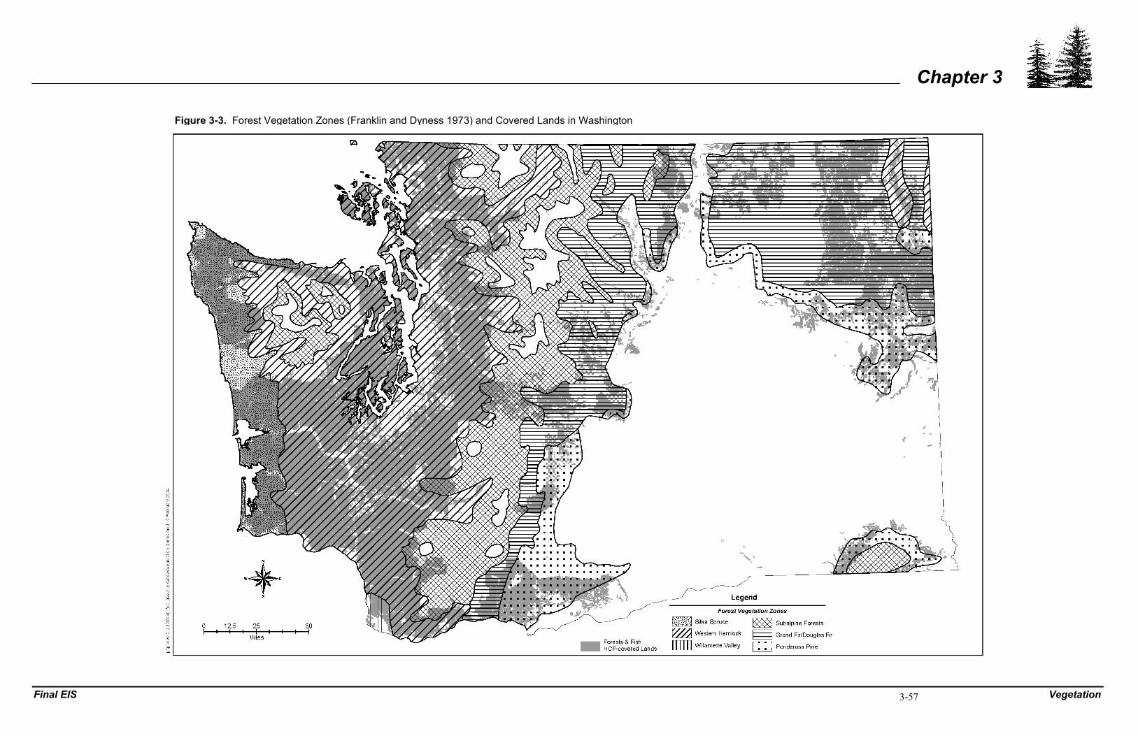
Final EIS Vegetation
Chapter 3
3-57
Figure 3-3. Forest Vegetation Zones
Figure 3-3
Figure 3-3. Forest Vegetation Zones (Franklin and Dyness 1973) and Covered Lands in Washington

This page is intentionally left blank.

Final EIS Vegetation
Chapter 3
3-59
lower elevation boundary is generally 4,900 feet in the Cascades and 4,200 to 5,600 feet in 1 other areas. Because covered lands generally lie at lower elevations, the subalpine forest 2 region encompasses a relatively small proportion of covered lands (626,000 acres or 3 6 percent of all covered lands). 4
Subalpine forests in Washington have wet, cool climatic regimes. Annual precipitation 5 averages between 55 and 110 inches and is strongly influenced by elevation. Much of the 6 precipitation falls as snow during the fall and winter months. Summers are cool and 7 winters are cold with snow cover persisting for up to 6 months, particularly in the 8 mountain hemlock zone. 9
Typical tree species in the Pacific silver fir zone include Pacific silver fir, western 10 hemlock, noble fir (Abies procera), Douglas-fir, western red-cedar, and western white pine. 11 The mountain hemlock zone is dominated by mountain hemlock, subalpine fir, and 12 lodgepole pine (Pinus contorta), while subalpine fir, Engelmann spruce (Picea 13 engelmannii), and lodgepole pine comprise the major tree species in the subalpine fir zone. 14
Douglas-Fir/Grand Fir Zones – The Douglas-fir and grand fir zones are found in eastern 15 Washington and generally lie above the drier ponderosa pine zone and below the subalpine 16 forests. These zones extend north from the Oregon-Washington border along the eastern 17 slopes of the Cascades and across north-central and northeastern Washington (Figure 3-3). 18 The Douglas-fir zone is typically found between 2,000 and 4,300 feet in northeastern 19 Washington. This zone is more mesic than the lower elevation ponderosa pine zone, with 20 cooler temperatures and higher annual precipitation. Douglas-fir, ponderosa pine, 21 lodgepole pine, and western larch (Larix occidentalis) comprise the major tree species in 22 the zone. Together, the Douglas-fir and grand fir zones encompass 2.1 million acres of 23 covered lands (19 percent of all covered lands). 24
The grand fir zone usually lies above the Douglas-fir zone and has the most moderate 25 environmental regime of any eastern Washington forest zone. Neither moisture nor 26 temperature conditions are extreme. Precipitation is generally higher and temperatures 27 lower than in lower elevation forest zones. Major tree species in the grand fir zone include 28 grand fir, ponderosa pine, lodgepole pine, western larch, and Douglas-fir. 29
Ponderosa Pine Zone – The ponderosa pine zone occupies three areas in Washington: 1) 30 a narrow band (10 to 20 miles wide) along the eastern flanks of the Cascade Range, 2) the 31 Blue Mountains, and 3) the Okanogan Highlands (Figure 3-3). The zone lies between 32 2,000 and 4,000 feet in elevation along the eastern flanks of the Cascades and between 33 3,000 and 5,000 feet in the Blue Mountains. Covered lands occur sporadically throughout 34 the ponderosa pine zone, encompassing 795,000 acres or 7 percent of all covered lands. 35
The ponderosa pine zone is characterized by a short growing season and minimal summer 36 precipitation. Average annual precipitation ranges from 14 to 30 inches, much of which 37 falls as snow during the winter months. Diurnal summer temperatures fluctuate widely, 38 with hot days and cold nights. Winter temperatures are generally low and snow often 39 accumulates to considerable depths. 40
Vegetation Final EIS
Chapter 3
3-60
Ponderosa pine is the climax species and is commonly associated with quaking aspen 1 (Populus tremuloides) and lodgepole pine throughout the zone. In the Okanogan 2 Highlands, grand fir, Douglas-fir, western larch, and western white pine are common 3 associates, while in south-central Washington, Oregon white oak is often present. 4
3.6.2 Riparian Vegetation 5 The vegetative communities that are commonly associated with riparian areas can be 6 divided into three general areas of Washington: forested areas in western Washington, 7 forested areas in eastern Washington, and the non-forested shrub-steppe region in eastern 8 Washington (Knutson and Naef 1997). For the purpose of this FEIS only forested riparian 9 areas are generally described. The species, sizes, and density of vegetation occupying a 10 riparian site are dependent upon soil moisture conditions and disturbance history. 11
Western Washington riparian habitats are associated with wet environmental conditions. 12 Although considerable site-specific variability occurs, general vegetative characteristics 13 include the presence of a mixture of conifer and hardwood trees (hardwoods are more 14 abundant where natural and human disturbance is frequent). Common conifers found in 15 riparian areas are western hemlock, western red-cedar, and Sitka spruce – species that are 16 tolerant of shade and periodically saturated soils. Red alder is nearly always found in 17 young and disturbed stands. Upland conifers (e.g., Douglas-fir) and hardwoods (e.g., 18 bigleaf maple) are dominant along small streams, which have narrow riparian areas. 19 Lowland rivers and forested swamps with frequent flooding or gravelly soils often include 20 black cottonwood, willow (Salix spp.), and red alder. Swampy areas may also have vine 21 maple (Acer circinatum), cascara (Rhamnus purshiana), willow, western red-cedar, Sitka 22 spruce, and western hemlock (Knutson and Naef 1997). Some of these species also are 23 common components of riparian areas on drier sites. 24
Forested riparian areas of eastern Washington are typically located in deeply incised 25 ravines in mountainous terrain (Carlson et al. 1990 in Knutson and Naef 1997). Lower 26 elevations with moist soils and temperate microclimates support cedar, western hemlock, 27 bigleaf maple, quaking aspen, and other hardwood trees. Large trees, snags, and downed 28 wood can be abundant in areas depending on disturbance history. These relatively moist 29 riparian areas also include a variety of understory shrubs and herbs including willow, red-30 osier dogwood (Cornus stolonifera), mountain alder (Alnus incana tenuifolia), devil’s club 31 (Oplopanax horridum), and other species. Drier sites are characterized by ponderosa pine 32 in the uplands while trees in riparian areas include Douglas-fir, paper birch (Betula 33 papyrifera), black cottonwood, and quaking aspen. High elevation riparian sites often have 34 saturated soils that are dominated by understory species rather than by tree species. Where 35 trees exist, they are commonly subalpine fir or Engelmann spruce and down wood is 36 abundant because cold temperatures slow decomposition. Shrubs and herbs at high 37 elevations are relatively diverse, but generally stunted due to the more severe 38 environmental conditions (Knutson and Naef 1997). 39

Final EIS Vegetation
Chapter 3
3-61
3.6.3 Disturbance Agents 1 Stand disturbance has long been a factor in Pacific Northwest forests. Disturbance factors 2 include fire, wind, insects, and pathogens. 3
3.6.3.1 Fire 4 Fire has been an integral part of the forest environment for thousands of years. The 5 likelihood of a fire initiation and the extent and severity of the resulting fire are affected by 6 the vegetation and other fuels on the site. The most common natural cause of forest fires is 7 lightning. Areas east of the Cascade crest average 10 to 15 thunderstorms per year, while 8 areas west of the Cascades average five per year. Most of the forested areas of Washington 9 experience between one and six lightning fires per 100,000 acres each year. Lightning 10 fires, which usually start as the result of lightning strikes in large trees or snags, account 11 for approximately 37 percent of the forest fires in Washington. Less than 1 percent is 12 caused by spontaneous combustion or other natural causes (Agee 1993). The remaining 13 fires are caused by humans, and are due to campfire escapes, industrial activity, other 14 accidents, or are intentionally set. When conditions are dry and fuel is abundant, fires can 15 burn large areas. One lightning fire in Chelan County, the 1994 Tyee Fire, burned more 16 than 140,000 acres. 17
In the cool, moist climate of western Washington, climatic conditions, fuel accumulation, 18 and lightning ignition historically have combined to result in infrequent extensive stand-19 replacement fires (fires that kill virtually all vegetation). These fires were generally more 20 intense than fires in eastern Washington and often resulted in a 50- to 100-year time span 21 before the burn area became fully restocked with native conifers (Franklin et al. 1981). 22 The historical natural fire return interval for cedar, spruce, and hemlock stands of western 23 Washington is about 937 years and about 217 years for Douglas-fir stands (Agee 1993). 24 Higher moisture levels found in riparian areas can increase fire return intervals in those 25 areas (Agee 1993). The return interval (cycle or turnover time) is the mean time between 26 disturbances on a given site. 27
Historically, fires in eastern Washington have been more frequent and less intense than 28 fires in western Washington, with ponderosa pine forests experiencing extensive fires 29 every 15 years on average, mixed conifer forests an average of every 50 years, and the 30 moister, high elevation forests experiencing fire only about once every 500 years (Agee 31 1993). Often the more frequent fires in eastern Washington represented understory burns 32 that maintained the canopy, or at least a portion of the canopy and were not stand 33 replacement fires where all vegetation would have been killed. These frequent lighter fires 34 in the ponderosa pine and Douglas-fir zones were instrumental in maintaining the open 35 pine forests noted by 19th century settlers. Natural disturbance from fire on the eastside is 36 an important factor defining stand seral stage characteristics under unmanaged condition 37 (Washington Forest Practices Board 2001a). 38
Fire control practices during the last century, in all areas of Washington, have increased the 39 fire intervals throughout the State (i.e., fires occur less frequently) (Agee 1993). These 40 increased fire intervals cause buildup of unnatural levels of dead and dying materials that 41 can fuel fires. This fuel buildup may results in more intense and frequent stand-42
Vegetation Final EIS
Chapter 3
3-62
replacement fires, particularly in eastern Washington. Currently, fuel levels are high in 1 many parts of eastern Washington because the frequent understory fires that once burned 2 these areas and kept fuel levels in check have been aggressively suppressed. These 3 frequent understory fires that historically occurred in eastern Washington helped maintain 4 natural ponderosa pine forests that were open and park-like because ponderosa pine is a 5 species that relies on high heat for natural regeneration of the species. The heat of forest 6 fires facilitates the opening of ponderosa pine cones allowing the seeds to disperse and 7 germinate. The reduction in forest fires in eastern Washington could be linked to a 8 reduction in the quantity of ponderosa pine forests. Management of a disturbance agent 9 such as fire, can itself cause a disturbance effect by altering types of vegetation present 10 (Washington Forest Practices Board 2001a). 11
3.6.3.2 Wind 12 Historically, windstorms have had a larger effect on westside forests than on eastside 13 forests, and fire has had a larger effect on eastside forests than on westside forests. Wind 14 has been especially potent in coastal Sitka spruce and high elevation Pacific silver fir and 15 alpine forests, where the moist conditions generally limited fire spread (Agee 1993). The 16 historic return intervals for windstorms in western Washington are approximately 119 to 17 384 years for small-scale to large-scale storms (Washington Forest Practices Board 2001a; 18 Harcombe 1986 as cited in Agee 1993). The 1921 windstorm and the Columbus Day 1962 19 windstorm blew down thousands of acres of mature trees in the western Olympic Peninsula 20 and other areas of western Washington (Washington DNR 2003). In addition to major 21 regional wind storms, locally intense winds are an important cause of small-scale 22 disturbance, which occurs across the landscape on an annual basis. 23
3.6.3.3 Insects and Pathogens 24 Insects and pathogens (fungi, viruses, dwarf mistletoe) are an important part of forest 25 ecosystems. They have many, complex biological roles and interactions. Insects and 26 pathogens may weaken or kill trees; stimulate altered tree growth forms such as forked 27 tops, galls, and bushy growths; affect light and heat reaching streams or the forest floor; 28 and cause a fertilization effect with feces. Insects act as pollinators, but also consume 29 seeds and fruit. Insects, fungi, and dwarf mistletoe plants are prey or food resources for 30 fish (Dodge 2001) and wildlife. The presence or absence of some insect species can give 31 indications of water quality characteristics. Mychorrhizal fungi enhance the uptake of 32 water and nutrients by roots. Saprophytic insects and fungi consume dead plant and animal 33 material, affecting the softness and longevity of snags, increasing soil quality, releasing 34 nutrients. 35
The effects of native insects and pathogens are considered to be part of how ecosystems 36 function. Damaged trees become nest sites for birds and salamanders and make space for 37 other trees and plants to grow. A root rot pocket may not grow Douglas-fir for the next 38 60 years, but the openings, scattered mortality, and increased volume of LWD may provide 39 big game forage, small animal habitat sources, increased diversity in plant communities, 40 and enhanced visual quality at the landscape scale (Theis and Sturrock 1995). Humans 41 may judge the activity of insects and pathogens in relation to their long- and short-term 42

Final EIS Vegetation
Chapter 3
3-63
management objectives for the land. Humans intervene or affect these interactions by 1 conducting management activities that control the trees species, structure, and vigor on a 2 site. Non-native insects and diseases, introduced by human activities, have the potential to 3 disrupt ecosystem balance and processes. Some examples of insect/pathogen and forest 4 interactions are described below. 5
Exotic Pest Species and Native Hosts Natural Defenses 6 The white pine blister rust fungus was introduced accidentally in the early 20th century. It 7 has killed vast numbers of native western white pine that produce heavy seed crops for 8 wildlife, once abundant and widespread in eastern and western Washington. This fungus 9 has now reached alpine areas where high losses to whitebark pine (Pinus albicaulis), a 10 critical food and habitat tree in this harsh environment, are expected (Baskin 1998; Goheen 11 et al. 2002). The balsam woolly adelgid, an introduced insect, is making grand fir more 12 susceptible to drought and insect defoliators, and will likely reduce the range of subalpine 13 fir (which die at low elevations, but survive in higher sites where it is too cold for the 14 insect to complete its lifecycle) (Mitchell 2001). The exotic defoliator, larch casebearer, 15 causes some damage to western larch, but has come somewhat into balance because 16 intentionally-introduced exotic predatory insects control it (Ryan 1997). The exotic 17 cinnabar moth was intentionally released in Washington and has successfully suppressed 18 populations of the tansy ragwort, a noxious weed that invades grassland habitats and is 19 toxic to animals that eat it (Washington State Noxious Weed Control Board 2004). 20
Fire Suppression and Insects/Pathogens 21 Humans have succeeded at suppressing almost all but the most severe and extreme forest 22 fires. Therefore, particularly in eastern Washington where light fires were more common, 23 without the thinning, clearing and diversity enhancing effects of fire, forests are more 24 dense, dominated by shade-tolerant species (Douglas-fir and grand fir replacing pine and 25 larch), and more uniform in structure than in the past. Weak, crowded trees are more 26 susceptible to being killed by bark beetles, particularly during times of drought 27 (Edmonds et al. 2000). Crowded trees in dense stands are excellent habitat for defoliating 28 caterpillars such as the western spruce budworm and Douglas-fir tussock moth (that feed 29 on Douglas-fir and true firs). Insect defoliator outbreaks are more frequent, last longer, 30 and cause more damage to affected trees than prior to European settlement (Hessburg et al. 31 1994). The dense forests are also more susceptible to root diseases and dwarf mistletoe 32 infection because close proximity of weak trees facilitates transmission of the pathogens. 33 Alternatively, the insect defoliators of mature pine trees have been less numerous, and 34 insect and wildlife species (such as the mardon skipper butterfly, an endangered butterfly 35 in Washington) that use the grasses and openings beneath pine trees have been reduced 36 (Hessburg et al. 1994; Potter et al. 1999). 37
Forest Fragmentation 38 Fire suppression and logging have affected the continuity of forests. While fire 39 suppression has made forests more uniform; logging has tended to break forest stands into 40 discrete units (although the uniformity within a stand may be increased as it is planted to 41 only one species with a relatively uniform spacing). The native defoliators, western spruce 42
Vegetation Final EIS
Chapter 3
3-64
budworm and Douglas-fir tussock moth, have benefited by the increase in forest density 1 and continuity that fire suppression has brought (Hessburg et al. 1994). 2
Forest Management and Pathogens 3 Native tent caterpillars benefit from edge habitat and hardwood-favoring disturbances that 4 logging and settlement have brought to Puget Sound. The white pine weevil thrives when 5 Sitka spruce are grown in large openings or plantations, in contrast to the partial shade they 6 probably grew in following fire or windthrow disturbances (Oregon Department of 7 Forestry 1999b; Hamid et al. 1995). Moreover, creation of stumps enhances many root 8 diseases. Root disease fungi persist in decaying underground root material and stumps 9 long after the infected tree has died or been removed. If the tree is cut, the root rot fungi 10 can persist in the buried portions of the stump for decades. If the tree tips over, then most 11 of the roots and stump are levered out of the ground and dry out, reducing fungus 12 inoculums on the site. Annosum root and butt rot invades trees when spores land on 13 wounds or cut stumps. Levels of Annosum root and butt rot were reduced when forest 14 managers initially removed very old, infected trees, but will increase with increasing 15 management activities that create stumps and basal wounds and maintain trees for longer 16 rotation ages (Schmitt et al. 2000). 17
Species Composition 18 Insects and pathogens have generally evolved to feed on a single or few closely-related 19 host tree species. Their activity levels are affected by the abundance of their host tree. For 20 example, the native foliar pathogen Swiss needle cast causes premature needle loss in 21 Douglas-fir (Southwest Oregon Forest Insect and Disease Service Center 2004). It is most 22 severe near coastal areas because the spores are protected by moist, foggy weather. Where 23 humans have replaced coastal hemlock forests with Douglas-fir plantations, the intensity of 24 Swiss needle cast disease has risen (Southwest Oregon Forest Insect and Disease Service 25 Center 2004). In contrast, the hemlock looper (caterpillar) feeds on the foliage of western 26 hemlock and associated conifers. It reaches high outbreak populations in old growth 27 hemlock forests with abundant moss and lichen for egg laying sites. 28
Snag and Downed Log Abundance 29 Snags and dead portions of trees are important nesting sites for woodpeckers and carpenter 30 ants, predators of bark beetles, and defoliating caterpillars. In many managed forests, 31 timber harvest, salvage logging (i.e., commercial harvest of dead, downed logs) and 32 firewood gathering have reduced the availability of snags and large logs, thus reducing 33 insect predators. The natural population cycles of the herbivorous insects may become 34 more intense, erratic, and damaging (Bull et al. 2001). Ants are an important food for 35 black bears when berries are scarce (Schowalter et al. and Withgott 2001). Logs may also 36 protect soil organisms from disturbances like fire, summer drought, and timber harvest. 37 Without sufficient numbers of logs, recolonization of disturbed soils could be slowed. 38 These soil organisms provide critical functions of nutrient cycling and soil aeration 39 (Schowalter et al. and Withgott 2001). 40
Final EIS Vegetation
Chapter 3
3-65
3.6.3.4 Special Problems in Eastern Washington Riparian Areas 1 Disturbance following European settlement has occurred primarily through timber harvest, 2 land clearing, agriculture, and, in some areas, fire. Much of Washington forestlands have 3 been logged at least once in the past 100 years (Washington DNR 2003). Generally, 4 timber was selectively logged (i.e., the removal of specific trees only) in eastern 5 Washington. As a result, eastern Washington riparian areas include dense understories, 6 dense reproduction, and more fire-intolerant species resulting in high fuel accumulation 7 and more intense and destructive fires as compared to natural conditions (Wissmar et al. 8 1994; Washington Forest Practices Board 2001a). 9
Riparian habitat disturbance factors include all of the above mentioned factors plus a few 10 additional factors in eastern Washington that can have significant impacts. These 11 disturbance factors include grazing, mining, and irrigation (DEIS Appendix A). Studies 12 have shown that livestock grazing within riparian areas eliminates or reduces streamside 13 vegetation, destabilizes streambanks, causes channel sedimentation and aggradation, 14 widens channels, increases stream temperature extremes, lowers the water table, reduces 15 bank undercut, and reduces pool frequency and depth (Armour et al. 1991; Chaney et al. 16 1993; Kauffman and Krueger 1984; Kovalchik and Elmore 1992; Meehan 1991; Platts 17 1991). Grazing pressure usually is higher in the riparian zone because there typically is 18 more shade, surface water for drinking, and more succulent vegetation than outside of 19 these zones (Platts 1991). 20
3.6.4 Threatened and Endangered Plants 21 The Washington DNR Natural Heritage Program maintains a list of threatened, 22 endangered, and sensitive plant species known to occur in each county. The list is derived 23 from a comprehensive Geographic Information System database of known occurrences of 24 threatened, endangered, and sensitive plants in the State (http://www.dnr.wa.gov/nhp/ 25 refdesk/plants.html). Many threatened, endangered, and sensitive plant habitats, such as 26 alpine, beach, exposed rock, or exposed grassy bluff, are not likely to be affected by 27 harvest or harvest-related activities. Other habitats such as meadows, prairies, or forest 28 openings may not support trees for harvest but may be adjacent to harvest areas and could 29 potentially be affected by harvest activities. The species that occur in forested habitats, 30 including microhabitats in forests such as forest openings, have a high likelihood of being 31 affected by harvest or harvest-related activities. Table 3-17 shows federally listed and 32 candidate plant species, their habitat, and distribution on covered lands by analysis region. 33 None of these species are intended to be covered by a take authorization under the FPHCP. 34
3.6.5 Invasive Plants 35 The historical emphasis of Washington State noxious weed law has been to protect the 36 economic interests of commercial agriculture in the State. While the effects of noxious 37 weed species on agriculture are large, their effects on the natural resources and ecological 38 diversity of the State are also large. These resources, once destroyed, may be irreplaceable. 39 Noxious weeds threaten not only agriculture, but also rangelands, waterways, parks, 40
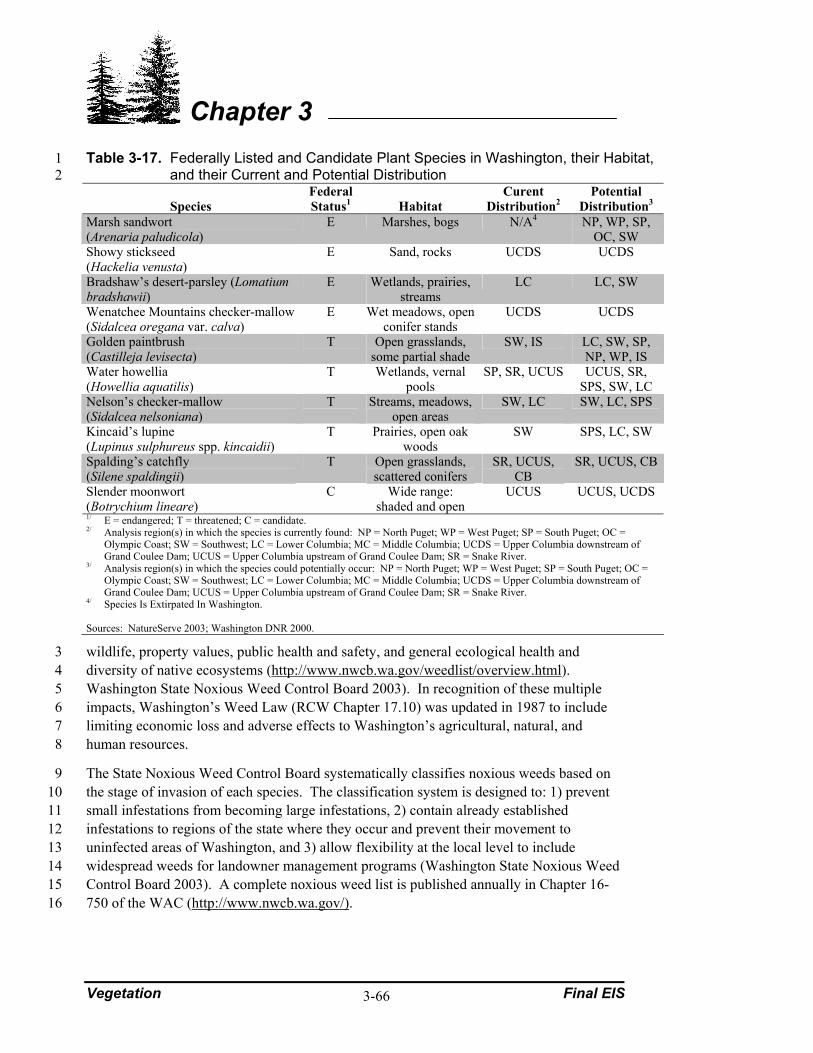
Vegetation Final EIS
Chapter 3
3-66
Table 3-17. Federally Listed and Candidate Plant Species in Washington, their Habitat, 1 and their Current and Potential Distribution 2
Species Federal Status1 Habitat
Curent Distribution2
Potential Distribution3
Marsh sandwort (Arenaria paludicola)
E Marshes, bogs N/A4 NP, WP, SP, OC, SW
Showy stickseed (Hackelia venusta)
E Sand, rocks UCDS UCDS
Bradshaw’s desert-parsley (Lomatium bradshawii)
E Wetlands, prairies, streams
LC LC, SW
Wenatchee Mountains checker-mallow (Sidalcea oregana var. calva)
E Wet meadows, open conifer stands
UCDS UCDS
Golden paintbrush (Castilleja levisecta)
T Open grasslands, some partial shade
SW, IS LC, SW, SP, NP, WP, IS
Water howellia (Howellia aquatilis)
T Wetlands, vernal pools
SP, SR, UCUS UCUS, SR, SPS, SW, LC
Nelson’s checker-mallow (Sidalcea nelsoniana)
T Streams, meadows, open areas
SW, LC SW, LC, SPS
Kincaid’s lupine (Lupinus sulphureus spp. kincaidii)
T Prairies, open oak woods
SW SPS, LC, SW
Spalding’s catchfly (Silene spaldingii)
T Open grasslands, scattered conifers
SR, UCUS, CB
SR, UCUS, CB
Slender moonwort (Botrychium lineare)
C Wide range: shaded and open
UCUS UCUS, UCDS
1/ E = endangered; T = threatened; C = candidate. 2/ Analysis region(s) in which the species is currently found: NP = North Puget; WP = West Puget; SP = South Puget; OC =
Olympic Coast; SW = Southwest; LC = Lower Columbia; MC = Middle Columbia; UCDS = Upper Columbia downstream of Grand Coulee Dam; UCUS = Upper Columbia upstream of Grand Coulee Dam; SR = Snake River.
3/ Analysis region(s) in which the species could potentially occur: NP = North Puget; WP = West Puget; SP = South Puget; OC = Olympic Coast; SW = Southwest; LC = Lower Columbia; MC = Middle Columbia; UCDS = Upper Columbia downstream of Grand Coulee Dam; UCUS = Upper Columbia upstream of Grand Coulee Dam; SR = Snake River.
4/ Species Is Extirpated In Washington. Sources: NatureServe 2003; Washington DNR 2000.
wildlife, property values, public health and safety, and general ecological health and 3 diversity of native ecosystems (http://www.nwcb.wa.gov/weedlist/overview.html). 4 Washington State Noxious Weed Control Board 2003). In recognition of these multiple 5 impacts, Washington’s Weed Law (RCW Chapter 17.10) was updated in 1987 to include 6 limiting economic loss and adverse effects to Washington’s agricultural, natural, and 7 human resources. 8
The State Noxious Weed Control Board systematically classifies noxious weeds based on 9 the stage of invasion of each species. The classification system is designed to: 1) prevent 10 small infestations from becoming large infestations, 2) contain already established 11 infestations to regions of the state where they occur and prevent their movement to 12 uninfected areas of Washington, and 3) allow flexibility at the local level to include 13 widespread weeds for landowner management programs (Washington State Noxious Weed 14 Control Board 2003). A complete noxious weed list is published annually in Chapter 16-15 750 of the WAC (http://www.nwcb.wa.gov/).16

Final EIS Riparian and Wetland Processes
Chapter 3
3-67
3.7 RIPARIAN AND WETLAND PROCESSES 1
3.7.1 Riparian Areas 2 Riparian habitat is the area adjacent to streams, rivers, lakes, and wetlands and includes 3 floodplains and stream-associated seeps and springs. A wide variety of hydrologic, 4 geomorphic, and biotic processes determine the character of riparian areas. Raedeke 5 (1988) describes riparian systems as having long, linear shapes with high edge-to-area 6 ratios and microclimates distinct from those of adjacent upland areas. Portions of riparian 7 areas are disturbed from periodic inundation, and water is present at or near the soil surface 8 during all or part of the year. These unique characteristics result in variable soil moisture 9 conditions and distinct plant, animal, and invertebrate communities that are often more 10 diverse than surrounding upland areas. 11
Riparian areas have distinct resource values and characteristics that make them important 12 zones of interaction between terrestrial and aquatic ecosystems (Knutson and Naef 1997). 13 These areas are especially dynamic segments of a watershed. Disturbance processes in 14 upland areas (e.g., fire, mass wasting, and windthrow), as well as disturbance processes 15 unique to stream systems (e.g., bank erosion, peak flows, floods) all affect riparian areas 16 (Benda et al. 1998; Montgomery and Wohl 20043; Spence et al. 1996; Reeves et al. 1995). 17 Functional riparian areas along streams and rivers in Washington are generally composed 18 of large conifers, or a mixture of large conifers and hardwoods and a diverse understory 19 plant community. Riparian vegetation is important for maintaining streambank and 20 floodplain integrity. Vegetation slows water velocity on the floodplain, and plant roots 21 inhibit erosion along streambanks, reducing sediment deposition in streams (subsection 22 3.4, Geology, Soils, and Erosion). Riparian vegetation also helps to provide shade, leaf 23 and needle litter important to aquatic food chains and nutrient cycling, and LWD, which is 24 an important component of instream fish habitat (subsection 3.8, Fish and Fish Habitat). 25 Riparian ecosystems are also important for a variety of plant and wildlife species. They 26 provide the primary habitat for many of the State’s amphibians (subsection 3.9, 27 Amphibians and Amphibian Habitat) and provide important reproductive and foraging 28 areas and/or dispersal/movement corridors for a wide variety of other wildlife (subsection 29 3.10, Birds, Mammals, Other Wildlife and Their Habitats). Clearing or harvesting trees 30 along streambanks and road construction near or adjacent to streams can negatively affect 31 riparian ecosystem functions (Chamberlin et al. 1991; FEMAT 1993; Spence et al. 1996). 32
This section summarizes the primary functions of the riparian area. In addition, it provides 33 a general description of the history of riparian management/riparian protection on private 34 and State lands in Washington and the current riparian conditions in Washington State. 35 Riparian vegetation was described in subsection 3.6.2 (Riparian Vegetation), and special 36 disturbance problems in eastern Washington riparian areas were described in subsection 37 3.6.3.4 (Special Problems in Eastern Washington Riparian Areas). 38
3.7.1.1 Riparian Functions 39 To understand the effects of various management actions, it is important to understand the 40 function of riparian areas, which have been described by many authors (e.g., Karr and 41

Riparian and Wetland Processes Final EIS
Chapter 3
3-68
Schlosser 1977; Meehan et al. 1977; Raedeke 1988; Bilby 1988; Murphy and Meehan 1 1991; Beschta 1991; Castelle et al. 19912). The most important recognized functions of 2 stream riparian areas include LWD recruitment, leaf and needle litter production, stream 3 shade, microclimate, streambank stability, groundwater recharge, stream energy 4 dissipation, and the routing and trapping of sediment. Streambank stability and sediment 5 filtration are introduced and evaluated in subsection 3.4 (Geology, Soils, and Erosion). 6 The other riparian functions (LWD recruitment, leaf and needle litter production, stream 7 shade, and microclimate) are briefly summarized below. 8
3.7.1.2 LWD Recruitment 9 Riparian areas are an important source of LWD that enters, or is recruited to, the stream 10 channel. LWD includes entire trees, rootwads, and larger branches. Numerous studies 11 have shown that LWD is an important component of fish habitat (Swanson et al. 1976; 12 Bryant 1983; Bisson et al. 1987; Naiman et al. 1992). Trees that fall into streams are 13 critical for sediment retention (Keller and Swanson 1979; Sedell et al. 1988), gradient 14 modification (Bilby and Ward 19891979), structural diversity (Ralph et al. 1994), nutrient 15 production (Cummins 1974), and protective cover from predators. LWD also creates 16 storage sites for sediment in all sizes of streams. In small headwater streams, wood 17 controls sediment movement downstream minimizing the risk of debris flows. In large 18 streams, accumulation of coarse sediment behind LWD often provides spawning gravels 19 (Bilby and Bisson 1998; Montgomery et al. 2003). LWD plays an important role in stream 20 nutrient dynamics by providing inputs of leaf litter and needles. 21
Large wood recruitment originates from a variety of processes including tree mortality, 22 windthrow, undercutting of streambanks, debris avalanches, deep-seated mass soil 23 movements, and redistribution from upstream (Swanson and Lienkaemper 1978). First and 24 second-order headwater streams can provide wood to larger higher order channels 25 downstream (Potts and Anderson 1990; Pritchard et al. 1998; Coho and Burges 1991). 26 Wood can be transported from upstream during high flow events and from debris torrents, 27 which includes dam-break floods and debris flows (Swanson and Lienkaemper 1978). 28 However, high flow events are more common in third- to fifth-order streams (See 29 Glossary) because much of the wood that falls into streams is too large to float in smaller 30 streams (Swanson and Lienkaemper 1978). Although less frequent than high flow events, 31 debris torrents can introduce large amounts of LWD (Lamberti et al. 1991). Debris flows 32 originating in managed forests (albeit, under older less protective rules) occur at a rate 33 much higher than that of unmanaged forests (Swanston and Swanson 1976; Morrison 34 1975). The majority of debris flows and dam-break floods are initiated in low order 35 streams, primarily second-order streams (Coho and Burges 1991). Debris flows can travel 36 upwards of 2.5 miles into higher order, low gradient valley floors, and cause substantial 37 damage to riparian vegetation and aquatic habitat during and after the event (Coho and 38 Burges 1991). The destructive impacts of debris torrents can be reduced by maintaining 39 contiguous riparian zones of mature conifers and minimizing deposition of logging slash 40 into and along low order channels (Coho and Burges 1991). Wood and coarse sediment 41 deposits from debris torrents can also form new habitat at tributary junctions by supplying 42

Final EIS Riparian and Wetland Processes
Chapter 3
3-69
LWD that forms pools, cover, channel complexity, and by supplying spawning gravel 1 (Benda et al. 2003). 2
The potential size distribution of LWD is also an important factor when considering the 3 appropriate activities in riparian buffers relative to LWD recruitment. LWD that is large 4 enough to form a pool is referred to as “functional LWD.” In contrast, “key piece LWD,” 5 a subset of “functional LWD,” is considered to be a better measure of the important wood 6 recruitment sizes. Key pieces are large and effective in trapping other smaller, more 7 mobile of LWD (i.e., forming logjams). Key pieces of LWD are also more likely to have 8 long-term stability (Bilby and Ward 1989; Collins et al. 2002; Hyatt and Naiman 2001). 9
Minimum functional LWD size increases with channel width (Bilby and Ward 1989; Bilby 10 and Wasserman 1989; Beechie and Sibley 1997; Beechie 1998; Washington Forest 11 Practices Board 1995). For example, mean LWD diameter increased from 11.7 inches in 12 westside channels, which were 5 feet wide, to 21.7 inches in channels 44 feet wide (Bilby 13 and Ward 1989). Key piece size is also related to stream size and is about 15 percent 14 larger in diameter than functional piece size for a 40-foot wide stream (Washington Forest 15 Practices Board 1995; Bilby and Ward 1989). As a result, riparian management zones 16 need to ensure not only an appropriate amount or volume of wood, but wood of sufficient 17 size to serve as both functional pieces and key pieces (Murphy 1995). Consequently, the 18 length of time needed for riparian areas to produce LWD after harvest depends upon the 19 size of the stream, stand composition, and site potential. Measurable contributions of 20 wood from second-growth riparian areas are documented to take anywhere from 60 to 250 21 years, depending on region and size of stream (Grette 1985; Bilby and Wasserman 1989; 22 Murphy and Koski 1989). Therefore, large streams that are deficient in LWD and have 23 adjacent and upstream riparian areas bordered by early seral stage riparian stands are likely 24 to remain deficient in LWD longer than smaller streams because of their requirement to 25 have large key pieces to retain LWD (MacDonald et al. 1991; Abbe and Montgomery 26 2003). However, if numerous key piece size LWD were available in these wide stream 27 reaches, and because LWD transport distance increases with stream size, these large 28 streams may be able to increase LWD locally by capturing downstream-transported LWD 29 in jams developed by key pieces (Abbe and Montgomery 2003; Martin and Benda 2001; 30 Collins et al. 2002). However, the development of key pieces of LWD is infrequent in 31 most early seral stage forests. 32
3.7.1.3 Leaf and Needle Litter Production 33 In aquatic systems, vegetative organic materials originate within the stream, such as algae 34 production, or from sources outside the stream, such as leaf and needle litter. Stream 35 benthic communities (e.g., aquatic insects) are highly dependent upon algal production and 36 detrital (i.e., organic debris) inputs. The abundance and diversity of aquatic species can 37 vary substantially depending upon the total and relative amounts of algae and leaf litter 38 inputs to a stream (Independent Multidisciplinary Science Team 1999). For example, 39 grazing insects are more commonly found in stream reaches with algae production, while 40 shredding insects are more commonly found in areas rich in leaf and needle input 41 (Independent Multidisciplinary Science Team 1999). Detrital input is the primary source 42 of organic productivity in heavily-shaded, small and medium size streams (Gregory et al. 43

Riparian and Wetland Processes Final EIS
Chapter 3
3-70
1991; Richardson 1992). In contrast, wide, high order streams with high levels of direct 1 sunlight, or low order streams with an open riparian canopy, have more algal production. 2 As a riparian stand ages, the amount of litter-fall increases (Independent Multidisciplinary 3 Science Team 1999). The importance of detrital input varies among streams, but can 4 provide up to 60 percent of the total energy input into stream communities (Richardson 5 1992). Small (low-order) streams are important sources of nutrients and contribute 6 substantially to the productivity of larger streams in the lower reaches of a watershed 7 (Independent Multidisciplinary Science Team 1999). 8
3.7.1.4 Stream Shade 9 There are several factors that make up the heat balance of water (subsection 3.5.1, Surface 10 Water Quality) including: air temperature, solar radiation, evaporation, convection, 11 conduction, and advection (Brown 19831980; Adams and Sullivan 1989). Stream 12 temperatures have a natural tendency to warm from upstream to downstream in the 13 watershed (Sullivan et al. 1990; Zwieniecki and Newton 1999). Seasonal and diurnal 14 variability also exists with stream temperatures. Other site-specific factors such as latitude, 15 regional climate/weather, stream size, groundwater inflow, and distance from watershed 16 divides all can affect stream temperature (Beschta et al. 1987; Sullivan et al. 1990). During 17 the summer when stream temperatures are the highest, the combination of warmer air 18 temperatures, increased direct solar radiation and decreased stream flows are the major 19 factors affecting stream temperature (Beschta et al. 1987). Of these three factors, forest 20 management can have the greatest effect on direct solar radiation by reducing shade. 21 Shade alone does not physically cool the stream, but it prevents further heating of the 22 stream and maintains the cool water temperatures from groundwater inputs or tributaries 23 (Oregon Forest Practices Advisory Committee on Salmon and Watersheds 2000). Shade 24 from riparian vegetation has been shown to minimize or eliminate increases in stream 25 temperature associated with timber harvest (Brazier and Brown 1973; Lynch et al. 1985). 26 Other factors that affect shading include local topography, stream size and aspect, stand 27 age, composition, and stand density. 28
3.7.1.5 Microclimate 29 Microclimate is a collection of variables that are highly dependent on local conditions; 30 hence, microclimates tend to vary greatly across the landscape. Important components of 31 microclimate include solar radiation, soil temperature, soil moisture, air temperature, wind 32 velocity, and air moisture or humidity (Chen 1991; Chen et al. 1992; Cadenasso et al. 33 1997). Changes in microclimatic conditions within the riparian zone resulting from 34 removal of adjacent vegetation can influence a variety of ecological processes that may 35 affect the long-term integrity of riparian ecosystems (Spence et al. 1996). For example, 36 many of the variables considered in microclimate studies (air temperature, humidity, wind 37 velocity) are also variables that affect water temperature (Sullivan et al. 1990), an 38 important component of fish habitat. Additionally, microclimate is known to be important 39 for aquatic/riparian species other than fish, such as amphibians (subsection 3.9, 40 Amphibians and Amphibian Habitat). In general, due to the low-lying position on the 41 landscape, riparian areas tend to be cooler than the surrounding hillslopes, especially 42 during the night. Because riparian areas are adjacent to water bodies, they often have a 43
Final EIS Riparian and Wetland Processes
Chapter 3
3-71
higher relative humidity under the canopy than upslope areas. This increase in humidity, 1 combined with shading effects, can result in forested riparian areas creating a moderating 2 effect on microclimate (Beschta 1991). 3
3.7.1.6 Historic Protection of Riparian Areas 4 The protection of riparian areas is considered critical to the long-term health of aquatic 5 ecosystems and salmonid conservation efforts (FEMAT 1993; Cederholm 1994; Murphy 6 1995). Riparian areas are protected by restricting management activities within the 7 riparian management zone (RMZ). Management within RMZs usually involves two main 8 features: 1) establishment of a buffer width, and 2) restrictions on allowable activities (e.g., 9 timber harvest prescriptions) within the buffer. Protection of water quality and fish habitat 10 is often given the highest management priority; however, buffers may also be designed to 11 benefit wildlife and other non-fish aquatic species. 12
Washington Forest Practices Rules have consistently been reviewed and revised in light of 13 new scientific information, changing public awareness, and evolving demands for forest 14 and water resources. The Washington State Forest Practices Act of 1974 created a Forest 15 Practices Board, which promulgates Washington Forest Practices Rules. Early riparian 16 rules only considered changes in stream temperature and bank stability for the aquatic 17 ecosystem. All riparian trees could be cut, sparing only the understory on certain 18 temperature-sensitive streams. Since then the Washington Forest Practices Rules have 19 undergone numerous revisions. Sweeping changes occurred in 1987 with the TFW 20 Agreement and rule changes resulting from that agreement. Significant revisions were also 21 made in 1992, 1996, and the most recent revisions, based on the FFR, in 2001 (subsection 22 1.3.1, Forest Practices Program, and subsection 2.3, Alternatives Analyzed in Detail). 23
3.7.1.7 Current Condition of Riparian Areas 24 Current riparian conditions on State and private lands are mostly a function of past forest 25 management practices, but natural phenomenon such as wildfire, blowdown, non-26 management related landslides, and disease have also contributed to conditions in many 27 areas. Because riparian protection rules are a relatively recent phenomenon in Washington 28 State (1982), the majority of riparian forests on State, private, and some Federal lands have 29 been logged at least once. Therefore, long-term changes to the riparian habitat character 30 have resulted from multiple forest practices over time. These changes to riparian habitat 31 structure include simplification of the plant community, both in species composition and 32 structure (Knutson and Naef 1997). Today it is believed that red alder dominates more 33 riparian sites in western Washington than was “typical” under natural disturbance regimes 34 (Washington Forest Practices Board 2001a; McHenry et al. 1998). 35
Two studies, described below, classified streamside vegetation into three seral stages to 36 present a picture of current riparian vegetation conditions. Seral stage provides a general 37 picture of riparian condition and quality. The two studies cannot be directly compared to 38 each other because each study used its own definitions, study area, and data 39 collection/analysis methods. One study sampled lands subject to Washington Forest 40 Practices Rules throughout Washington, while the other study area was specific to western 41

Riparian and Wetland Processes Final EIS
Chapter 3
3-72
Washington riparian areas. Both studies, however, provide information that indicates the 1 current general condition of Washington’s riparian areas. 2
The first study was conducted to provide information for the recent Forest Practices 3 Alternatives SEPA EIS (Washington Forest Practices Board 2001a). Table 3-18 presents 4 the percentage of streamside vegetation on private lands subject to Washington Forest 5 Practices Rules that existed in the three seral stages (based on a random sample of lands). 6 Seral stages were based on tree sizes as follows: 7
• Early Seral – Reproduction, confer pole, hardwood pole, and mixed pole; less than 12 8 inches in diameter at breast height (dbh). 9
• Mid-Seral – Conifer sawtimber, hardwood sawtimber, and mixed sawtimber; 12 to 24 10 inches in dbh. 11
• Late Seral – Large conifer sawtimber, large hardwood sawtimber, and large mixed 12 sawtimber; greater than 24 inches in dbh. 13
The Forest Practices Board study concluded that unnaturally high levels of early seral stage 14 vegetation existed in riparian zones on private forestland, primarily as a result of timber 15 management activities and, to a lesser extent, from fire, blowdown, and other natural 16 processes in riparian areas (Washington Forest Practices Board 2001a). In general, early 17 seral stages produce riparian vegetation that provides lower riparian values for aquatic and 18 terrestrial biota. In contrast, later seral stages that are typically more diverse in species 19 composition and stand structure can more fully provide for riparian functions (e.g., shade 20 and LWD recruitment for aquatic biota) (subsection 3.8, Fish and Fish Habitat) and more 21 complex vegetative structure (e.g., downed logs and snags for terrestrial biota associated 22 with riparian habitat) (subsection 3.9, Amphibians and Amphibian Habitat, and subsection 23 3.10, Birds, Mammals, Other Wildlife and Their Habitats). 24
These data indicate that within the lands subject to Washington Forest Practices Rules up 25 to 2001, approximately 78 percent of western Washington stream miles and 61 percent of 26 eastern Washington stream miles flow through early seral stage riparian areas, while about 27
Table 3-18. Estimated Percent of Each Seral Stage along Forested Streams on 28 Private Lands. 1/ 29
Seral Stage - Percent by Water Type (%) Water Type Early Mid Late
Westside-Private Lands Types 1-3 64 33 2 Types 4-5 81 18 1
All Streams 78 21 1 Eastside- Private Lands
Types 1-3 60 36 4 Types 4-5 61 33 6
All Streams 61 34 5 Source: Washington Forest Practices Board 2001a, Appendix C, Table 6. Based on a random sample of private lands
(See DEIS Appendix B for a description of the sampling). See text for seral stage definitions. 30

Final EIS Riparian and Wetland Processes
Chapter 3
3-73
1 percent of western Washington miles and 5 percent of eastern Washington miles are late 1 seral. Though natural variability is expected in riparian areas, the level of alteration due to 2 timber harvest and road building is apparent. 3
The second study (Lunetta et al. 1997) used digital elevation modeling of stream channels 4 to determine channel gradient, and then characterized riparian seral stage by gradient 5 category. The analysis looked at forest vegetation in 179 watersheds across western 6 Washington. Stream channels were classified into three categories based on channel slope: 7 response reach, transport reach, and source reach. The response reach seral stage data are 8 the only raw data still available from this study and is, thus, the only data reported here. 9 Response reaches were defined as channel reaches with less than 4 percent slope, and were 10 considered the area where most anadromous fish production occurs. 11
Riparian response reaches were broken into three seral stages defined as follows: 12
• Early Seral – Hardwood dominated, shrub, or recent clearcut. Also includes forests 13 with greater than or equal to 10 percent and less than 70 percent conifer crown cover, 14 and less than 75 percent of total crown cover in hardwood tree/shrub cover. 15
• Mid-Seral – Forests with greater than 70 percent conifer crown cover, less than 10 16 percent crown cover in trees greater than or equal to 21 inches dbh. 17
• Late Seral – Forests with greater than 70 percent conifer crown cover, more than 10 18 percent of the crown cover must be in trees greater than 21 inches dbh. 19
Response reach seral stage data are summarized by analysis region in Table 3-19. Again, 20 as of 1997, the most common seral stage was early seral, ranging from 52 percent in the 21 West Puget Sound Region to 72 percent in the Lower Columbia Region. Late seral made 22 up the lowest percentage, ranging from 5 percent in the Southwest and South Puget Sound 23 Regions to 19 percent in the North Puget Sound Region. 24
Riparian condition and function (e.g., floodplain condition, bank stability, LWD, shade and 25 stream temperature, water quality) vary from good to poor within each region, depending 26 on site scale and location. For a more detailed analysis, see the Regional Summaries in 27 DEIS Appendix A. 28
3.7.2 Wetlands 29 Wetlands are defined in terms of their physical, chemical, and biological characteristics, 30 such as hydrologic regime, soil type, and plant species. Wetlands are formally defined as 31 those areas that are inundated or saturated with surface or groundwater at a frequency and 32 duration sufficient to support, and that under normal circumstances, do support a 33 prevalence of vegetation typically adapted for life in saturated soil conditions (40 CFR 34 230.41(a)(1); WAC 222-16-11). This definition includes forested swamps, marshes, bogs, 35 and other similar areas. Wetlands are subject to regulation through the Clean Water Act by 36 the U.S. Army Corps of Engineers and EPA. Sections 404 and 401 of the Clean Water Act 37 were created specifically with the intent “to restore and maintain the chemical, physical, 38 and biological integrity of our nation’s waters.” 39

Riparian and Wetland Processes Final EIS
Chapter 3
3-74
Table 3-19. Estimated Percent of Each Seral Stage along Response Reaches of 1 Forested Streams for Western Washington Analysis Regions. 2
Seral Stage Early Mid Late
Analysis Region (Acres/Percent)
Conifer Crown Cover Between 10
and 70%
Greater than 70% Conifer Canopy;
10% or Less of the Canopy in Conifers
Greater than 21”dbh
Greater than 70% Conifer Canopy;
More than 10% of the Canopy in
Conifers Greater than 21”dbh
Acres 55,704 17,323 16,808 North Puget Sound Percent 62 19 19
Acres 34,829 18,613 2,938 South Puget Sound Percent 62 33 5
Acres 27,416 17,994 7,157 West Puget Sound Percent 52 34 14
Acres 47,897 26,226 14,869 Olympic Coast Percent 54 29 17
Acres 103,810 46,893 8,582 Southwest Percent 65 29 5
Acres 69,833 17,421 10,080 Lower Columbia Percent 72 18 10
Source: Personal Communication, Brian Cosentino, Washington Department of Fish and Wildlife, October 2003.
3
Wetland ecosystems provide a variety of physical and biological functions. Additionally, 4 they provide many values to society including recreation, water quality enhancement, and 5 flood attenuation. The National Wetland Policy Forum (Conservation Foundation 1988) 6 identified eight natural functions that wetlands may perform at a landscape level. These 7 eight functions are: 1) nutrient removal and transformation, 2) sediment and toxicant 8 retention, 3) shoreline and bank stabilization, 4) flood flow alteration, 5) groundwater 9 recharge, 6) nutrient export, 7) aquatic diversity and abundance, and 8) wildlife diversity 10 and abundance. Values to society include recreation, water quality enhancement, and flood 11 control. 12
3.7.2.1 Wetland Functions 13 As noted above, wetlands provide a variety of functions and values. The key wetland 14 functions that are the focus of this FEIS include fish and wildlife habitat, water quality, and 15 hydrology. These functions were chosen because they may be most directly impacted by 16 timber harvest related activities. The functions are briefly discussed below. 17

Final EIS Riparian and Wetland Processes
Chapter 3
3-75
Fish and Wildlife Habitat 1 Wetland and riparian habitats are considered to be among the richest zones for aquatic and 2 terrestrial organisms (Dodd 1978; Brinson et al. 1981; Kauffman and Krueger 1984). 3 Because wetland and riparian habitats exhibit an “edge effect” due to overlapping types of 4 habitats, these areas provide more niches than are provided by any other habitat types. 5 Eighty-six percent (359 out of 414) of the terrestrial vertebrate species in western 6 Washington, and 85 percent (320 out of 378) of terrestrial vertebrate species in eastern 7 Washington utilize wetland and associated riparian habitats for portions of their life needs 8 (Brown 1985; Thomas 1979). 9
Wetlands provide habitat or perform functions that contribute to the health of ecosystems 10 of many anadromous and resident fish species within Washington. Wetlands are known to 11 help maintain cool water temperatures, retain sediments, store and desynchronize flood 12 flows, maintain stream base flows, and provide food and cover for fish (Cederholm and 13 Scarlett 1981; Beechie et al. 1994; Mitsch and Gosselink 1993; Washington Department of 14 Ecology 1993b1997). 15
Water Quality 16 Wetlands can improve water quality through nutrient removal and transformation 17 (Hammer 1989). For example, wetlands can remove nitrate and phosphorus from 18 agricultural runoff. Nutrient-rich sediments may also become trapped and removed from 19 the water. Wetlands can also remove toxic chemicals, such as pesticides, heavy metals, or 20 excess nutrients from water (Mitsch and Gosselink 1993). Wetlands can reduce shoreline 21 and bank erosion by binding soil substrates in wetland plant roots. Thus, wetlands protect 22 upland habitats along streams and rivers from erosion, and protect downstream habitats 23 from sedimentation and pollution. Wetlands, which discharge cool groundwater, can help 24 maintain desirable stream temperatures in the summer. Forested riparian and wetland areas 25 serve an important role in shading streams from direct solar heating. Other wetlands, 26 without cool groundwater discharge, may be a source of warmer water to stream 27 temperatures, but they also provide fish habitat and a source of nutrients. 28
Hydrology 29 Headwater riverine and depressional wetlands can delay discharge of peak run-off into 30 streams and impede passage of overbank flow downstream during storm events, thus 31 reducing the potential for downstream flooding (Winter 1988; Roth et al. 1993). 32 Depressional wetlands can help maintain minimum stream base flow by naturally 33 regulating the release of groundwater discharge into streams and by recharging aquifers 34 that discharge groundwater to streams (Dinicola 1990; Hidaka 1973; O’Brien 1988; Mitsch 35 and Gossselink 1993). 36
3.7.2.2 Historic/Current Wetland Protection 37 Wetlands are subject to regulation under Sections 401 and 404 of the Clean Water Act. 38 Discharge into wetlands may also be regulated under Section 402 of the Clean Water Act. 39 Exemptions granted under Section 404(f)(1) allow for normal agricultural, ranching, and 40 silvicultural activities, as well as maintenance of existing drains, farm ponds, and roads. 41
Riparian and Wetland Processes Final EIS
Chapter 3
3-76
The construction or maintenance of forest roads for silvicultural purposes is exempt from 1 regulation when such roads are constructed and maintained in accordance with BMPs. 2
On State and private lands in Washington, the Washington Forest Practices Rules provide 3 wetland resource protection from timber harvest-related activities. For management 4 purposes, the Washington Forest Practices Rules recognize two major categories of 5 wetlands: forested and non-forested. Non-forested wetlands are divided further into two 6 classes: Type A (greater than 0.5 acre, with open water) and Type B (other non-forested 7 wetlands). The Washington Forest Practices Rules require buffers, termed Wetland 8 Management Zones, on all Type A wetlands and most Type B wetlands. Harvest may 9 occur in forested wetlands; however, harvest methods are limited to low impact harvest or 10 cable systems. 11
For Type A wetlands greater than 5 acres in size, an average Wetland Management Zone of 12 100 feet is required. For Type A wetlands between 0.5 and 5 acres, a 50-foot average 13 Wetland Management Zone is required. For Type B wetlands greater than 5 acres, a 50-14 foot average Wetland Management Zone is required. For other wetlands between 0.5 and 5 15 acres, a 25-foot Wetland Management Zone is required. Wetlands less than 0.5 acre have 16 no buffer requirement. 17
In addition to leaving Wetland Management Zones, there are several other harvest 18 restrictions around non-forested wetlands. For example, individual trees and small patches 19 of forested wetlands (0.5 acre) cannot be harvested if surrounded by a Type A or Type B 20 wetland. Harvest of upland areas or large forested wetlands require a plan approved by 21 Washington DNR if they are surrounded by Type A or Type B wetlands. Additionally, 22 timber cannot be felled into or cable-yarded across a Type A or Type B wetland without 23 prior approval by Washington DNR. 24
3.7.2.3 Historic and Current Conditions of Wetlands 25 Since the time of colonization, Washington State has lost between 30 to 50 percent of its 26 wetlands (USFWS 1999). Additionally, the functions of existing wetlands have been 27 reduced. Various factors have contributed to wetland loss and wetland function reduction 28 including agriculture development, urbanization, timber harvest, road construction, and 29 other land management activities. It is difficult to assess the current condition of wetlands 30 in forested lands across the entire State of Washington. However, some wetlands on lands 31 subject to Washington Forest Practices Rules have been altered in the past due to timber 32 harvest and road building. These actions can impact wetland sites directly through 33 vegetation alteration, soil compaction, changes in hydrologic regime, and degradation of 34 water quality; or indirectly through sedimentation from adjacent land management 35 practices. Additionally, harvest of trees in or adjacent to wetland sites can impact the 36 associated microclimate (Brosofske et al. 1997; Chen et al. 1995, 1999). Other impacts to 37 wetlands have likely occurred from fires and other natural disturbances. 38
Washington DNR wetland GIS coverage was used to generate the data reported in Table 3-39 20. Overall, approximately 4.4 percent of the forestland base subject to the Washington 40 Forest Practices Rules evaluated is comprised of wetland habitats, based on this mapping. 41

Final EIS Riparian and Wetland Processes
Chapter 3
3-77
Wetland areas comprise approximately 2 percent of the land base in eastern Washington 1 and approximately 6 percent in western Washington. 2
Table 3-20. Approximate Wetland Area as a Percentage of Forested 3 Ownership, by Region and Wetland Type. 4
Region Ownership Type A
Wetland (%) Type B
Wetland (%) Other Open Water (%)
Forested Wetland (%)
Westside Private Lands 0.7 <0.1 <0.1 5.7
Eastside Private & State Lands
0.4 <0.1 <0.1 1.2
Statewide Private and State on Sampled lands
0.6 <0.1 <0.1 3.8
Note: < = less than
Source: Washington Forest Practices Board 2001a, Section 3.5.2.3, Table 3.5-1. Based on a random sample of lands subject to Washington Forest Practices Rules in each area/ownership category.
5

Riparian and Wetland Processes Final EIS
Chapter 3
3-78
This page is intentionally left blank. 1
2

Final EIS Fish and Fish Habitat
Chapter 3
3-79
3.8 FISH AND FISH HABITAT 1
3.8.1 Introduction 2 Fish are an important natural resource with both biological and economic significance in 3 the State of Washington. In particular, Pacific salmon and trout, as well as other fish 4 species, are indicators of a properly functioning aquatic ecosystem because they require 5 cool, clean water, complex channel structures and substrates, and low levels of silt (Bjornn 6 and Reiser 1991). In addition, Pacific salmon and trout support economically important 7 commercial and sport fishing industries, as well as subsistence fishing by many 8 Washington Indian Tribes. 9
This section discusses the fish species in Washington and their habitats. A complete list of 10 all species that are intended to be “covered” by the FPHCP is provided in Table 1-1. 11 Chapter 3 of the FPHCP presents life history and status information for all of these species. 12 Those fish species with the more critical Federal status of “endangered” or “threatened” are 13 given the most attention within this section; however, other fish species with less critical 14 Federal or State status are also described. Further, this section describes important 15 components of the aquatic environment that fish require and that forest practices may 16 effect. These components include water quality, water quantity, channel conditions, LWD, 17 channel morphology, and fish passage. 18
The following subsections emphasize the affected environment for fish species on State 19 and private lands within Washington State, which are regulated by Washington Forest 20 Practices Rules. The discussion contains a review of fish distribution and status within the 21 12 analysis regions defined in subsection 3.1 (Introduction). This section also contains a 22 review of important components of the aquatic ecosystem upon which fish rely for 23 sustaining healthy, well-dispersed populations. 24
3.8.2 Fish Status in Washington 25 More than 70 species of freshwater fish are present in the more than 8,000 lakes and 26 50,000 miles of streams within Washington (Wydoski and Whitney 2003). Generally, at 27 least one fish species is found in perennial streams with gradients less than 20 percent 28 (Fransen et al. 1997). Occasionally, fish are found in streams with steeper gradients, but 29 these circumstances are less common. Land-use practices upstream of fish-bearing waters 30 can affect downstream fish habitat. Consequently, the affected environment for fish 31 includes both fish-bearing and non-fish-bearing streams. 32
Two of the four goals of the Forest Practices Board for the Washington Statewide Salmon 33 Recovery Strategy (Washington Forest Practices Board 1999) have special reference to fish 34 and forestry interactions. One of the goals is to provide compliance with the Endangered 35 Species Act (ESA) for aquatic and riparian-dependant species on all lands subject to the 36 Forest Practices Act. A second goal is to restore and maintain riparian habitat on these 37 forestlands to support a harvestable supply of fish. 38
Notably, NMFS has not listed any Pacific salmon or trout species as threatened or 39 endangered throughout their entire range, because many populations within the entire range 40

Fish and Fish Habitat Final EIS
Chapter 3
3-80
are considered healthy or at least stable. Instead, NMFS has listed specific salmon and 1 trout stocks based upon distinct populations that are “substantially reproductively isolated” 2 and “represent an important component in the evolutionary legacy of the species” (Waples 3 1991). NMFS has termed these populations “Evolutionarily Significant Units.” 4 Analogously, the USFWS has chosen to use the term “Distinct Population Segments” for 5 freshwater fish species under its regulatory authority. 6
Beginning in 1991 with the listing of Snake River sockeye salmon by NMFS, the ESA has 7 increasingly affected the way government agencies and public and private landowners 8 conduct business in or near the streams and rivers found in the State. The rate of new 9 listings escalated in the late 1990s such that at least one Evolutionarily Significant Unit of 10 all of the Pacific salmon species, with the exception of pink salmon, have been listed as 11 threatened or endangered within one or more areas of Washington State (Table 3-21). In 12 addition to the Pacific salmon and trout listed by NMFS, the USFWS has listed bull trout 13 throughout its range in the contiguous United States. Consequently, there are few areas 14 within Washington State that do not have at least one listed fish species (Figures 3-4 15 through 3-9). 16
3.8.3 Life History of Covered and Affected Fish Species 17 A basic understanding of the life history and habitat requirements of the various covered 18 fish species is important for recognizing the type and level of effects that may result from 19 forest practices. The life history characteristics can vary substantially in different locations 20 depending on climate, food supply, stream flow, and other factors (Flosi and Reynolds 21 1994). 22
3.8.3.1 Pacific Salmon and Trout - General 23 The life cycle of anadromous Pacific salmon and trout can be divided into seven distinct 24 phases or life stages: upstream migration, spawning, egg incubation, fry emergence, 25 juvenile rearing, smolt outmigration, and marine rearing. Two important common 26 denominators in the life history of Pacific salmon and trout is they all construct redds 27 (nests) in gravel beds for spawning, and they all include life history forms that exhibit 28 anadromy. In other words, spawning occurs in freshwater, followed by migration to the 29 ocean for feeding and maturation, and finally fish return to their natal sites for completion 30 of the life cycle. Four of the salmon and trout species also have life history forms that live 31 their entire lives in freshwater (i.e., sockeye/kokanee, steelhead/rainbow, cutthroat, and 32 bull trout). Several anadromous species demonstrate extremely complex variations in 33 length of freshwater rearing, use of lake systems, run timing, degree of anadromy, and age 34 structure. These variations, in conjunction with geographically separate spawning 35 populations, have led to the stock concept of salmon management (Larkin 1972). It is the 36 demonstration of unique behavioral patterns, physical characteristics, and ultimately 37 genetic makeup that has made it possible to list any salmon stock within the framework of 38 the ESA (Nehlsen et al. 1991; Waples 1991). 39

Final EIS Fish and Fish Habitat
Chapter 3
3-81
Table 3-21. Covered Fish Species with Federal or State Listed Status in Washington State.
Species Population1/ Federal Status State Status Distribution 2/
Hood Canal Summer–run Threatened Candidate 5 Chum Salmon Oncorhynchus keta Columbia River Threatened Candidate 3
Puget Sound—Strait of Georgia Species of Concern
None 1, 4-7
Lower Columbia River Candidate None 3 Coho Salmon O. kisutch
Southwest Washington Species of Concern
None 2
Snake River Endangered Candidate 12 Sockeye Salmon O. nerka Ozette Lake Threatened Candidate 1
Snake R. Fall-run Threatened Candidate 12 Snake R. Spring/Summer-run Threatened Candidate 12
Puget Sound Threatened Candidate 4, 5, 7 Lower Columbia River Threatened Candidate 3, 9 Upper Willamette R. Threatened Candidate 9
Chinook Salmon O. tshawytscha
Upper Columbia River Spring-run Endangered Candidate 8 Upper Columbia River Endangered Candidate 8
Snake River Threatened Candidate 12 Lower Columbia River Threatened Candidate 3,9
Upper Willamette Threatened Candidate 9
Steelhead Trout O. mykiss
Middle Columbia River Threatened Candidate 9 Columbia River Threatened Candidate 3, 8-10, 12 Bull Trout
Salvelinus confluentus Coastal - Puget Sound Threatened Candidate 1, 2, 4, 5, 7 Coastal Cutthroat Trout O. clarki clarki
Species of Concern
None 1-7
Westslope Cutthroat Trout O. clarki clarki
Species of Concern
None 8-10, 12
Interior Redband Trout
Species of Concern
None 8-10, 12
Green Sturgeon Acipenser medirostris
Species of Concern
None 2-5, 7
Pacific Lamprey Lampetra tridentatae
Species of Concern
None 1-5, 8, 9, 12
River Lamprey L. ayresi
Species of Concern
Candidate 3-5, 7, 9, 12

Fish and Fish Habitat Final EIS
Chapter 3
3-82
Table 3-21. Covered Fish Species with Federal or State Listed Status in Washington State (continued).
Species Population1/ Federal Status State Status Distribution 2/
Margined Sculpin Cottus marginatus
Species of Concern
Sensitive 12
Pygmy Whitefish Prosopium coulteri
None Sensitive 1, 4, 8-10
Olympic Mudminnow Novumbra hubbsi
None Sensitive 1, 2, 4, 5
Umatilla Dace Rhinichthys Uumatilla
None Candidate 8-10
Leopard Dace R. falcatus
None Candidate 3, 8, 9
Lake Chub Couesius plumbeus
None Candidate 10
Eulachon Thaleichthys pacificus
None Candidate 1-3, 7
Mountain Sucker Catostomus platyrhynchus
None Candidate 3, 8, 9, 12
Salish Sucker C. carli
None Monitor 4, 5, 7
Sandroller Percopsis transmontana
None Monitor 3, 8-10, 12
1/ Populations of Pacific salmon are designated as Evolutionarily Significant Units (ESU) by NMFS. The USFWS designates threatened and endangered population segments as Distinct Population Segments (DPS).
2/ Numbers indicate EIS Regions where species occurs. Region: 1 = Olympic Coast; 2 = Southwest; 3 = Lower Columbia; 4 = South Puget Sound; 5 = West Puget Sound; 6 = Islands; 7 = North Puget Sound; 8 = Upper Columbia (downstream Grand Coulee); 9 = Mid Columbia; 10 = Upper Columbia (upstream Grand Coulee); 11 = Columbia Basin; 12 = Snake River.

Final EIS Fish and Fish Habitat
Chapter 3
3-83
Figure 3-4. Distribution and ESA Status of Chinook Salmon within Washington 1 State (Source: Streamnet, http://www.streamnet.org Version 99.1; 2 NMFS - http://www.nwr.noaa.gov/1salmon/Salmesa). 3
Figure 3-5. Distribution and ESA Status of Chum Salmon within Washington 4 State (Source: Streamnet, http://www.streamnet.org Version 99.1; 5 NMFS – http://www.nwr.noaa.gov/1salmon/Salmesa). 6
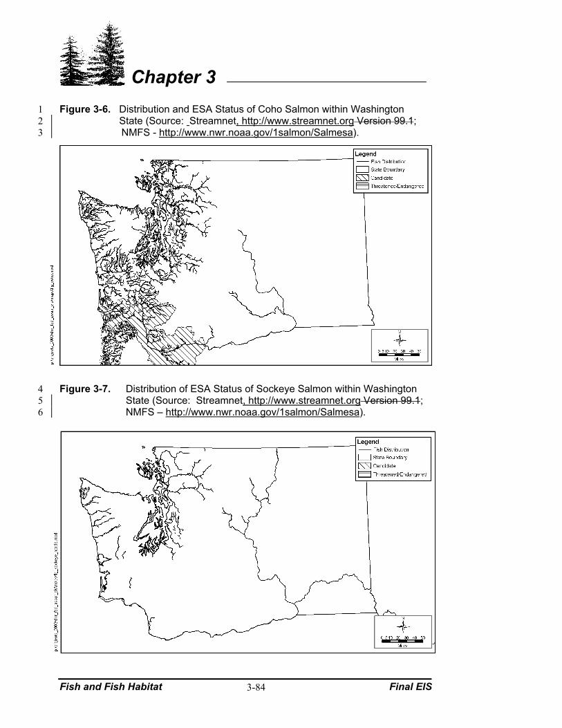
Fish and Fish Habitat Final EIS
Chapter 3
3-84
Figure 3-6. Distribution and ESA Status of Coho Salmon within Washington 1 State (Source: Streamnet, http://www.streamnet.org Version 99.1; 2 NMFS - http://www.nwr.noaa.gov/1salmon/Salmesa). 3
Figure 3-7. Distribution of ESA Status of Sockeye Salmon within Washington 4 State (Source: Streamnet, http://www.streamnet.org Version 99.1; 5 NMFS – http://www.nwr.noaa.gov/1salmon/Salmesa). 6

Final EIS Fish and Fish Habitat
Chapter 3
3-85
1 Figure 3-8. Distribution and ESA Status of Steelhead within Washington State 2
(Source: Streamnet, http://www.streamnet.org Version 99.1; NMFS - 3 http://www.nwr.noaa.gov/1salmon/Salmesa). 4
Figure 3-9. Distribution and ESA Status of Bull Trout within Washington State 5 (Source: Streamnet 2002, http://www.streamnet.org; USFWS Draft 6 Recovery Plan 2004b). 7

Fish and Fish Habitat Final EIS
Chapter 3
3-86
One commonly recognized variation in life history traits for Pacific salmon and steelhead 1 is run timing. The seasonal stock distinctions are based upon the date individual stocks of 2 maturing adults enter freshwater. For example, chinook salmon are often divided into 3 “spring,” “summer,” and “fall” runs, while steelhead stocks are divided into “winter” and 4 “summer” runs. Sockeye usually do not have multiple distinct runs and the seasonal 5 descriptor is often omitted. Most pink salmon in the Puget Sound Region enter freshwater 6 during the fall while sockeye salmon runs peak in early July. Chum salmon exhibit 7 summer, fall, and winter run timing. 8
Additional stock and species-specific variability is demonstrated in the duration of 9 freshwater rearing and the type of habitat that is utilized. Spring chinook salmon, coho 10 salmon, and steelhead juveniles typically spend 1 or 2 years rearing in streams prior to 11 outmigration. Similarly, sockeye salmon usually spend a year rearing in a lake prior to 12 outmigration. In contrast, ocean-type chinook and chum, and pink salmon outmigrate to 13 the ocean as fry. Chum salmon usually complete their outmigration shortly after 14 emergence (Wydoski and Whitney 2003), while fall chinook may have a protracted 15 outmigration period that occurs throughout the summer (Dawley et al. 1986). While most 16 summer/fall chinook outmigrate during their first year, a small proportion overwinter in 17 freshwater and then migrate as yearlings the following spring. 18
Bull trout and coastal cutthroat trout also express high variability in migratory behavior 19 and habitat use. They have four different migratory forms: anadromous, adfluvial, fluvial, 20 and resident. Adfluvial stocks rear in lake systems, but migrate to tributary streams for 21 spawning. Fluvial stocks rear entirely in larger streams or rivers, but have lengthy 22 migrations between headwater spawning and rearing areas. Other trout subspecies such as 23 westslope cutthroat and redband trout are solely resident and do not exhibit anadromy. 24 Though resident stocks demonstrate little “migratory” behavior (compared with 25 anadromous fish), connectivity is critical throughout their specific habitat ranges in order 26 to fulfill all of their life history needs (i.e., spawning, rearing, foraging, escaping extreme 27 environmental fluctuations, and recolonization after habitat disturbance). 28
For freshwater spawning and rearing, salmon and trout (as well as other freshwater fish 29 species) have life-stage and species-specific habitat requirements. Important components 30 to spawning habitat include substrate size, water depth, and water velocity (Bjornn and 31 Reiser 1991). In general, the larger species utilize larger substrates and deeper and faster 32 water (0.5 to 4 in. [1.3 to 10.2 cm], greater than 9 in. [24 cm] depth, 1.1 to 3.6 ft/sec [32 to 33 109 cm/sec] velocity) (Bjornn and Reiser 1991). Tail-outs to pools (the downstream end 34 where the pool changes to a riffle) that meet criteria for these features are generally 35 considered optimal spawning areas for salmonids because stream morphology maximizes 36 the passage of oxygenated water through redds. Chums commonly utilize spring or 37 groundwater upwelling areas for spawning (Salo 1991). However, runs, riffles, and 38 groundwater or spring upwelling zones along lakeshores and intertidal sloughs are also 39 utilized during spawning. Redd building is important for three principal reasons (Chapman 40 1988): 1) redds provide physical protection to eggs during periods when they are extremely 41 fragile; 2) redd digging removes a portion of the fines and sands deleterious to egg 42

Final EIS Fish and Fish Habitat
Chapter 3
3-87
survival; and 3) redd construction and morphology enhances the passage of water through 1 the egg pockets. 2
Following emergence from the redd, salmon and trout fry typically utilize shallow and 3 slow moving areas of a stream (Bjornn and Reiser 1991). Optimal depths and velocities 4 increase as the fish grow, but preferred areas are usually associated with some form of 5 cover, usually pools with LWD or boulders, or with faster water areas. Differences among 6 the species are apparent in the degree of flexibility for utilizing riffles, runs, and other 7 habitat features. Stream dwelling juvenile salmonids are typically territorial and exhibit a 8 dominance hierarchy among individuals and species. Drifting insect larvae and benthic 9 macroinvertebrates account for the majority of food items eaten by juvenile salmon and 10 trout within streams. In contrast to the typical stream dweller, sockeye fry migrate to a 11 lake shortly after emergence where shallow nearshore (or littoral) areas are preferred 12 habitat. As sockeye fry grow, they begin to move offshore and have a characteristic 13 diurnal vertical migration timed for utilization of zooplankton food sources (Bjornn and 14 Reiser 1991; Burgner 1968; Groot and Margolis 1991; Wydoski and Whitney 2003). 15
Riparian areas have distinctive resource values and characteristics that are critical to 16 salmonid production (FEMAT 1993). Riparian vegetation is important for maintaining 17 streambank and floodplain integrity. The vegetation slows water velocity on the floodplain 18 and roots inhibit erosion along streams and riverbanks, which reduces sediment deposition 19 in streams. Riparian vegetation also helps to provide shade (important for the maintenance 20 of stream temperatures), leaf, and needle litter important to aquatic food chains and LWD 21 (FEMAT 1993). Riparian vegetation and LWD also traps and retains salmon carcasses, an 22 important source of marine-derived nitrogen (Bilby et al. 1996). 23
In general, the marine phase of salmonid life history is not well understood. Only recently 24 have ocean environmental conditions been considered an important factor in the 25 management of salmon resources (Bisbal and McConnaha 1999). Historically, the ocean 26 was assumed an unlimited resource for salmon production, but this assumption is now 27 being widely questioned. Forest practices are likely to have very minimal direct effects on 28 anadromous fish once they are in the marine environment, since many other factors such as 29 tides, currents, nutrients, marine food sources, marine predators, become paramount in 30 their growth and survival. However, forest practices may affect woody debris and 31 sediment composition and supply in estuarine and nearshore environments, which have the 32 potential to affect rearing and migratory life stages (Simenstad et al 2003; Maser and 33 Sedell 1994; Washington Department of Fish and Wildlife 1997; Collins et al. 2002). 34
The following subsections provide a life history for each of the covered species considered 35 in this FEIS, beginning with those species having federally listed status. See FPHCP 36 Chapter 4 (Life History, Status, Distribution and Factors Affecting Covered Species) for 37 additional descriptions of species characteristics. 38
Chum Salmon 39 Within Washington State, two populations of chum salmon are federally listed as 40 threatened (i.e., Hood Canal summer chum and Columbia River chum). Chum salmon, 41

Fish and Fish Habitat Final EIS
Chapter 3
3-88
also known as dog salmon and/or calico salmon, are distinguished by the reddish purple 1 vertical markings along the sides of spawning adults. In the Pacific Northwest, freshwater 2 migration is typically short (less than 50 miles). Chum salmon utilize the low gradient (0 3 to 8 percent) reaches of the stream, sometimes tidally influenced, for spawning, but the 4 nearshore and estuarine areas are known to be early rearing areas for many salmonid 5 species (Groot and Margolis 1991; Wydoski and Whitney 2003). The estuarine area is a 6 transition zone for acclimation from fresh to marine water and commonly a feeding area 7 for early stages of many fish. These regions, estuaries and nearshore areas, are also 8 spawning and rearing areas for many of the baitfish species that are often food sources for 9 these early and later stages of salmonids. Chum fry typically spend less than 30 days in 10 freshwater after emergence but remain in the estuary and nearshore environments as 11 juveniles, feeding primarily on copepods, tunicates, and euphausids prior to migrating out 12 to the ocean (Lichatowich 1993). Chum return to freshwater in 3 to 5 years to spawn and 13 tend to be group spawners with each female accompanied by one or more males. Chum 14 salmon carcasses, as well as the other salmon species, provide a food source for juvenile 15 salmonids and numerous wildlife species. The abundance of chum salmon tends to 16 fluctuate during even/odd cycles, suggesting a possible competitive interaction with pink 17 salmon, where present in estuary or nearshore habitats (Salo 1991). 18
Chum salmon have three distinct run times: summer, fall, and winter (late fall). Summer 19 chum begin their upstream migration and spawning during low summer flows in mid-20 August through mid-October with fry emergence ranging from the beginning of February 21 through mid-April, depending on water temperatures (Washington Department of Fish and 22 Wildlife (WDFW) and Point No Point Treaty Tribes 2000). Fall chum adults enter the 23 rivers in late October through November, and spawn in November and December. Winter 24 chum adults migrate upstream from December through January and spawn from January 25 through February. Fall and winter chum fry emerge from the gravels in March and April 26 and quickly outmigrate to the estuary for rearing (Smith 1999). 27
Coho Salmon 28 One population of coho (Lower Columbia River) is a Federal candidate species within 29 Washington State. Coho, also known as silver salmon, are distinguished by black spots on 30 the upper part of the caudal fin and a white mouth. Coho begin their upstream migration 31 between September and December, penetrate deep into the upper watersheds, generally 32 spawn from October through February, and emerge in early March to late July. Most 33 juvenile coho remain at least 1 year in freshwater; although recent studies have shown that 34 some populations spend time in estuaries prior to smoltification. Those that remain in 35 freshwater typically spend the summer months rearing in pools or other low-velocity 36 habitats. Many juvenile coho migrate to off channel habitats such as wetlands or side 37 channels, during winter, a strategy that provides protection from severe winter flows. They 38 school for a brief period after emerging from gravel, but later disperse and become 39 aggressive and territorial (Smith 1999). 40
Streams with more structure (logs/rootwads, boulders, undercut-banks) support more coho, 41 not only because they provide more territories/usable habitat, but they also provide more 42 food and cover (Scrivener and Andersen 1982). There is a positive correlation between 43
Final EIS Fish and Fish Habitat
Chapter 3
3-89
their primary diet of insect material and the extent the stream is overgrown with vegetation 1 (Chapman 1965). During the winter, coho often feed on adult salmonid carcasses (Bilby et 2 al. 1996). As coho juveniles grow into yearlings, they become more predatory on other 3 salmonids. Coho go through physiological changes preparing for life in salt water, and 4 migrate to sea in spring (Lichatowich 1993). They typically spend 2 years at sea and return 5 as 3-year-old adults. Coho use estuaries primarily for interim food while they adjust 6 physiologically to saltwater and then move offshore to deeper waters (Smith 1999). 7
Sockeye Salmon 8 Within Washington State, two populations of sockeye salmon are federally listed: Snake 9 River Sockeye are listed as endangered (they spawn in Redfish Lake, Idaho and migrate 10 within the Columbia River) and Ozette Lake Sockeye are listed as threatened. Sockeye, 11 also known as red salmon, are distinguished as spawning adults by their red bodies and 12 green heads as well as lack of spots on the back or caudal fin. Sockeye enter freshwater for 13 upstream migration during the summer months, spend time resting in deep pools or lakes, 14 and enter the spawning grounds when ready to spawn. Sockeye are unique in that they 15 exhibit three life history strategies: one type spawns in rivers but rears in lakes for 1 to 16 3 years to complete their freshwater life cycle prior to migrating out to sea (lacustrine-17 adfluvial); one type spawns along lake shores and rears in lakes for 1 to 3 years prior to 18 migrating out to sea (lacustrine); and one less common type spawns and rears in rivers and 19 streams (fluvial). 20
Incubation time varies from 50 days to 5 months, depending on water temperature. After 21 emerging, lake-rearing fry find their way to a nursery lake, where they feed on insects, 22 larvae, and copepods. Juvenile sockeye spend up to 3 years in freshwater prior to 23 smoltification in spring; although some populations outmigrate immediately upon 24 emergence and others may remain in freshwater for their entire lives (e.g., kokanee). 25 Migrating sockeye juveniles remain within the estuarine/nearshore environment throughout 26 the summer, feeding on insects, crustaceans, and small fish and their larvae. Sockeye grow 27 and develop for 2 to 4 years in the ocean prior to returning to their natal stream to spawn 28 (Wydoski and Whitney 2003). 29
Chinook Salmon 30 Within Washington State, Upper Columbia spring chinook salmon are federally listed as 31 endangered. Chinook in the Snake River, Puget Sound, Lower Columbia River, and upper 32 Willamette River are listed as threatened. Chinook salmon, also known as king salmon, 33 are distinguished as adults by black spots on both lobes of the caudal fin and black gums 34 along the lower jaw. At maturity (4 to 5 years average), chinook seek out spawning 35 grounds, which can extend from just above tidal influence to as far as 1,200 miles upstream 36 (Wydoski and Whitney 2003). Spawning habitat preferences include deeper water and 37 larger gravels than for most other salmon (Healey 1991). 38
Run timing, when adults return to the freshwater to spawn, can occur during spring, 39 summer, or fall, depending upon particular stock and river system. Spring chinook adults 40 begin river entry in May or early June and spawn from July through September, typically 41 in headwater areas with higher gradient habitat. Incubation continues through autumn and 42
Fish and Fish Habitat Final EIS
Chapter 3
3-90
winter, generally requiring additional development time due to the colder water 1 temperatures of the headwaters. Adult summer chinook begin river entry as early as June 2 and spawn from September through October. Fall chinook stocks range in spawn timing 3 from late September though December. Chinook juveniles incubate in the gravel until 4 January through early March. After emerging from the gravel, juveniles rear in fresh water 5 from a couple of months to a couple of years. Outmigration of smolts to the marine 6 environment occurs over a broad period, typically January through August (Smith 1999). 7 Time is spent within estuarine and nearshore environments prior to entering the ocean. 8
While some emerging chinook fry outmigrate quickly, most inhabit the shallow side 9 margins and side sloughs for up to two months. At this time, some gradually move into the 10 faster water areas of the stream and/or disperse into tributaries for rearing, while others 11 outmigrate to the estuary. Most summer and fall chinook outmigrate within their first year 12 of life, but a portion of some stocks remain in the river an additional year. Spring chinook 13 stocks, which rear in colder water and often further upstream, typically rear at least a year 14 in fresh water (Marshall et al. 1995). However, for Washington populations, Columbia 15 River Chinook stocks, other than Hanford Reach fall Chinook salmon and a few others, are 16 primarily river type (with extended freshwater residence), while coastal and Puget Sound 17 populations exhibit a variable river and ocean life history (with short-term freshwater 18 rearing). 19
Steelhead 20 Within Washington State, Upper Columbia Steelhead are federally listed as endangered. 21 Steelhead within the Snake River and Lower and Middle Columbia River, and Upper 22 Willamette River steelhead are listed as threatened. Steelhead are distinguished by their 23 uniform silvery color until darkening toward spawning time. They are the anadromous 24 form of rainbow trout. Unlike Pacific salmon, steelhead may return to sea after spawning 25 and migrate again to freshwater to spawn again another year. There are two races of 26 steelhead: summer and winter. While there is some overlap, winter run steelhead typically 27 enter streams for spawning between November and April, while stream-maturing summer 28 steelhead enter streams between May and October (Wydoski and Whitney 2003). Summer 29 steelhead usually spawn further upstream than winter stocks and dominate inland areas 30 such as the Columbia Basin. The coastal streams in western Washington typically support 31 more winter steelhead populations (Smith 1999). 32
Steelhead juveniles typically spend 1 to 2 years (rarely 3 years) in fresh water, preferring 33 riffle areas in the summer and occupying pools during the rest of the year (Wydoski and 34 Whitney 2003). During the winter, they often feed on the carcasses of adult salmonids 35 (Bilby et al. 1996). Steelhead migrate to sea in the spring, spending up to 4 years in the 36 open ocean (Wydoski and Whitney 2003), feeding on crustaceans, squid, herring, and other 37 fish (Lichatowich 1993). 38
Bull Trout/Dolly Varden 39 Bull trout are federally listed as threatened throughout their range. Until 1978, bull trout 40 and Dolly Varden, both native char, were considered the same species. They were 41 eventually separated based on morphometrics, osteological features, and embryological 42

Final EIS Fish and Fish Habitat
Chapter 3
3-91
development. Bull trout inhabit both eastern and western Washington State, while Dolly 1 Varden inhabit only Puget Sound and coastal rivers west of the Cascades. Bull trout and 2 Dolly Varden exhibit four life history strategies: anadromous, adfluvial, fluvial, and 3 resident. 4
Anadromous forms move upstream in late summer and early fall to spawn in September 5 and October, or in November at higher elevations (Wydoski and Whitney 2003). All types 6 of bull trout and Dolly Varden prefer clean, cold water (50°F [10 °C]) for spawning 7 (Oregon Department of Environmental Quality 1995) and even colder water (36 to 39°F [2 8 to 4 °C]) for incubation (Rieman and McIntyre 1993). Extended incubation periods (up to 9 220 days) make bull trout eggs and fry particularly susceptible to increases in fine 10 sediments (USFWS 1998a). Fry are typically found in shallow, backwater side channels 11 and eddies in proximity to instream cover (Pratt 1984), juveniles in interstitial spaces in the 12 substrate, and subadults in deeper pools in streams or in the deep water of lakes with 13 temperatures less than 59°F (15 °C) (Pratt 1992). Bull trout mature at approximately 5 14 years, typically reproduce in alternate years (Armstrong and Morrow 1980; USFWS 15 1998a) and live for 12 or more years. Migratory forms of bull trout (anadromous and 16 fluvial) are known to move between fresh water and marine water and between natal 17 (spawning and rearing fresh water) and non-natal (habitat outside of their spawning and 18 rearing habitat) waters, particularly to find forage and overwinter (USFWS 2004b). 19
Resident bull trout and Dolly Varden exhibit three life history strategies, each with unique 20 habitat requirements: adfluvial, fluvial, and resident. Adfluvial bull trout rear as juveniles 21 in tributaries, migrate to lakes where most of their growth occurs, then return to the 22 tributaries as adults to spawn. Fluvial bull trout spawning occurs in smaller tributaries with 23 major growth and maturation occurring in river mainstems. Resident bull trout complete 24 all life stages (spawning, rearing, overwintering) in small headwater streams, often 25 upstream of barriers to other salmonids (USFWS 2004b). 26
Cutthroat Trout 27 The coastal sea-run cutthroat trout and the westslope cutthroat trout are two subspecies of 28 cutthroat trout native to Washington State. Both subspecies are Federal species of concern. 29 Only the coastal sea-run cutthroat trout is anadromous, but it also exhibits fluvial, 30 adfluvial, and resident life history forms. The westslope cutthroat, which predominately 31 occurs in major watersheds of eastern Washington, has only fluvial, adfluvial, and resident 32 life history forms. 33
Coastal cutthroat trout spawn in the cooler waters of the smallest headwater streams and 34 tributaries used by any salmonid species, and the young usually remain in these streams 35 about a year before moving down into larger streams. They live in these larger streams for 36 another 2 to 5 years (usually 3) before migrating to the Pacific Ocean (Wydoski and 37 Whitney 2003). Some stocks remain as residents of small headwater tributaries, or migrate 38 only into rivers or lakes (Scott and Crossman 1973). Sea-run cutthroat do not migrate to 39 the open ocean; rather, they stay in estuarine habitats near the mouths of their natal streams 40 for 5 to 8 months of the year. Upstream migration to freshwater feeding/spawning areas 41 occurs from late June through March. Re-entry timing is consistent from year to year 42

Fish and Fish Habitat Final EIS
Chapter 3
3-92
within streams, but varies widely between streams. Spawning generally occurs between 1 December and May in pool tailouts located in streams with low gradient and low flows or 2 in shallow riffles (Wydoski and Whitney 19792003). 3
Historically within Washington State, westslope cutthroat were distributed in two adjacent 4 river basins (Lake Chelan and Methow) in the mid-Columbia River drainage and the 5 headwaters of the Pend Oreille River in northeastern Washington (Williams 1999 as cited 6 within Wydoski and Whitney 2003). However, over the years, hatchery westslope 7 cutthroat have been introduced throughout eastern Washington as well as a few streams on 8 the westside of the Cascades. Genetically pure populations have been identified in various 9 pristine headwater streams and alpine lakes within eastern Washington; however, 10 inventories are not complete. Adfluvial westslope cutthroat spend 1 to 4 years as juveniles 11 in tributary streams before moving into lakes to rear. These adult cutthroat move back into 12 tributaries during high stream flows and spawn between March and July; however, they 13 return to the lake habitat shortly after spawning. Fluvial westslope cutthroat move from 14 tributary streams to mainstem habitat. Overwintering occurs in deeper pools and beaver 15 ponds. The resident life history of westslope cutthroat is similar to that of resident coastal 16 cutthroat (Wydoski and Whitney 2003). 17
Interior Redband Trout 18 Interior redband trout are a Federal species of concern. Native redband trout are the non-19 anadromous inland subspecies of rainbow trout. Although redband trout appear to be 20 widely distributed within the Columbia River Basin, their status is clouded by the 21 uncertainty over taxonomic classification within the species and by more than a century of 22 stocking hatchery rainbow trout and steelhead. Little published information exists for 23 redband trout in Washington State. Oregon status reports have described some life history 24 traits. In some basins, fluvial and adfluvial redband trout migrate upstream in the spring 25 and spawn in their respective basins from April to July depending upon elevation. Most 26 resident fish spawn in the spring and summer (Oregon Department of Fish and Wildlife 27 1999). 28
3.8.3.2 Green Sturgeon 29 The green sturgeon is a Federal species of concern. It is known to spawn in only three 30 river basins outside of Washington State (Klamath, Rogue, and Sacramento), leaving it 31 vulnerable to a catastrophic event. Freshwater habitats used by sturgeon are generally 32 large and deep. With the exception of a few landlocked populations, green sturgeon spend 33 most of their time in marine waters, moving into fresh water only to spawn (Scott and 34 Crossman 1973; Setter and Brannon 1992). Physical characteristics of green sturgeon eggs 35 suggest that the species probably requires cold, clean water for spawning and probably do 36 not spawn in Washington waters (Moyle et al. 1995). Green sturgeon have been reported 37 as far as 140 miles inland in the Columbia River, but are presently restricted to areas below 38 Bonneville Dam, and are found almost exclusively in the lower 40 miles of the river 39 (Moyle et al. 1995; Wydoski and Whitney 2003). The Columbia River estuary and other 40 coastal Washington estuaries appear to attract concentrations of green sturgeon during late 41 summer and early fall. Neither feeding nor spawning occurs in association with these 42

Final EIS Fish and Fish Habitat
Chapter 3
3-93
concentrations, and there is no information about how much of the population is in these 1 concentrations each year, or whether this varies (Adams et al. 2002). 2
3.8.3.3 Pacific and River Lamprey 3 Pacific and river lamprey are both Federal species of concern. Pacific lamprey populations 4 in the upper Columbia and Snake River basins have declined dramatically, likely as a result 5 of elevated water temperatures, sedimentation of spawning gravels, and barriers to 6 migration (Close et al. 1995). Population declines of the Pacific lamprey have prompted 7 concern for the river lamprey. In Washington, the Pacific lamprey is found in most large 8 coastal and Puget Sound rivers and occurs long distances inland in the Columbia, Snake, 9 and Yakima River systems (Lee et al. 1980; Wydoski and Whitney 2003). River lamprey 10 are found in coastal streams and estuaries and inland in the Columbia River to the 11 Columbia Gorge (Kostow 2002; Wydoski and Whitney 2003). Both lamprey are 12 anadromous and parasitic. Pacific lamprey enter freshwater between July and October. 13 They gradually move upstream to spawn the following spring (Hart 1973). Eggs hatch in 2 14 to 4 weeks (19 days at 59°F [15 °C]); newly hatched ammocoetes (larvae) remain in their 15 nests for 2 to 3 weeks before drifting downstream and burying themselves in mud at the 16 bottom of pools, or other areas of soft mud and sand (Hart 1973; Moyle 1976). Increased 17 water flows during runoff can also encourage outmigration by washing away the sand and 18 silt that the larvae require for anchoring themselves to the bottom (Hardisty and Potter 19 1971). 20
Little is known regarding the habitat requirements of the river lamprey. Adults migrate 21 into deep freshwater habitats in the fall. They spawn in the winter and spring in clean 22 gravel areas of small tributaries and die after spawning (Moyle et al. 1995). Based on 23 comparisons with other lamprey species, Hart (1973) surmised that river lamprey 24 ammocoetes (larvae) remain in their natal streams for several years, usually in silt-sand 25 backwaters and eddies near the bank. 26
3.8.3.4 Margined Sculpin 27 Margined sculpin have no Federal listing, but are a Washington State sensitive species. 28 They are found in the Walla Walla, Touchet, and Tucannon Rivers. Margined sculpin are 29 predominantly found in pools and glides but are also observed in riffles. They prefer small 30 gravels and silts, avoiding larger gravels and cobble. They reach an average length of 31 about 2.5 inches and probably live to be 4 years old. Spawning occurs in spring under 32 rocks, rootwads, or logs (Wydoski and Whitney 2003). 33
3.8.3.5 Pygmy Whitefish 34 Pygmy whitefish have no Federal listing, but are a Washington State sensitive species. 35 Pygmy whitefish are members of the trout and salmon family (Salmonidae) and are 36 typically around 5 to 6 inches in length when mature, reaching a maximum length of about 37 11 inches. The pygmy whitefish is a remnant species from the last ice age with a spotty 38 distribution across northern North America and in the Columbia River drainage in 39 Washington. The pygmy whitefish inhabits cold lakes and streams. Streams inhabited by 40 pygmy whitefish may be of moderate to swift current and may be silty or clear (Hallock 41 and Mongillo 1998). The pygmy whitefish has been eliminated from a minimum of 42

Fish and Fish Habitat Final EIS
Chapter 3
3-94
40 percent of its range in Washington. Historically, pygmy whitefish were known to have 1 occupied 15 lakes in Washington; however, today they are currently found in only 9 2 (Hallock and Mongillo 1998). The future of pygmy whitefish populations in Washington 3 is dependent upon our ability to maintain water quality, spawning habitat, and prevent 4 introduction of new predator species. Additionally, pygmy whitefish populations are 5 especially vulnerable to local extinction because natural reintroduction of new fish is 6 usually impossible among isolated lake systems. 7
3.8.3.6 Olympic Mudminnow 8 Olympic mudminnows have no Federal listing, but are a Washington State sensitive 9 species. They are found only in slow-moving streams, wetlands, and ponds with soft mud-10 bottom substrate, little or no water flow, and abundant aquatic vegetation (Harris 1974; 11 Mongillo and Hallock 1999; Wydoski and Whitney 2003). Species distribution is limited 12 to low gradient, low elevations in the coastal lowlands of the Olympic Peninsula, the rivers 13 of the Chehalis and lower Deschutes drainages, and south Puget Sound lowlands west of 14 the Nisqually River (Mongillo and Hallock 1999; Wydoski and Whitney 2003). The 15 species is considered vulnerable due to its limited distribution and dependence on healthy 16 wetland habitat (Mongillo and Hallock 1999). Wydoski and Whitney (2003) observe that 17 mudminnows are usually found under overhanging banks or shore vegetation, preferring 18 areas with low light and brownish water of bogs and swamps. Meldrim (1968) found a 19 wide tolerance for temperature extremes and low oxygen levels, but a restricted tolerance 20 range for salinity and water current. Adults spawn between November and June (peaking 21 in April and May) and females deposit eggs amidst clumps of vegetation, to which fry 22 remain firmly attached for approximately one week after hatching (Meldrim 1968 and 23 Hagen et al. 1972 in Mongillo and Hallock 1999). 24
3.8.3.7 Umatilla Dace and Leopard Dace 25 Neither the Umatilla nor leopard dace have Federal listing status; however, they are both 26 classified as Washington State candidate species. Concern for these species is prompted 27 by their restricted distribution as well as their preference for shallow water, which may 28 increase their vulnerability to activities that affect water levels (Royal British Columbia 29 Museum 1995). Two other species of dace (Longnose and speckled dace) also occur in 30 Washington State and share many key life history characteristics, such as breeding habitat, 31 spawning period, and habitat associations of juveniles. Dace typically occur in shallow 32 waters with cobble or gravel substrate (Scott and Crossman 1973; Troffe 1999; Wydoski 33 and Whitney 2003). Spawning generally occurs from late spring through summer 34 (Wydoski and Whitney 2003). Currently, relatively little information is available about the 35 Umatilla dace. At one time, this species was considered to be a stable hybrid between 36 leopard dace and speckled dace and, to date, is not a “recognized species in the United 37 States by the American Fishery Society. The taxonomic status is still open to debate” 38 (Personal Communication, Molly Hallock, Washington Department of Fish and Wildlife, 39 October 2003). The Umatilla dace is endemic to the Columbia River basin (Troffe 1999). 40 In Washington, it is known only from the larger main rivers of the basin, including the 41 Columbia River at Rock Island Dam and elsewhere in the Columbia River east of the 42 Cascades (Royal British Columbia Museum 1995). 43

Final EIS Fish and Fish Habitat
Chapter 3
3-95
The leopard dace is a Columbia River system fish, found west of the Cascade Mountains in 1 the Lower Columbia and the Cowlitz River system (Personal Communication, Molly 2 Hallock, Washington Department of Fish and Wildlife, October 2003) as well as in the 3 Columbia River system east of the Cascade Mountains (Scott and Crossman 1973; 4 Wydoski and Whitney 2003). 5
3.8.3.8 Lake Chub 6 Lake chub have no Federal status, but are a Washington State candidate species. In 7 Washington, they are known only from the northeastern part of the State (Wydoski and 8 Whitney 2003). Lake chub exhibit a variety of habitat preferences across their range, 9 living in large rivers at northern latitudes, but using lake habitat when it is available (Isaak 10 et al. 2003; Scott and Crossman 1973). In the southern portion of their range, the lake 11 chub is uncommon in lakes; but whether this represents a habitat preference or is simply 12 because fewer lakes are available is unknown (Isaak et al. 2003). The only known 13 Washington populations are in Cedar Lake in Stevens County (1998 observation) and in 14 North Fork Beaver Creek in Okanogan County (1999 observation; Personal 15 Communication, Molly Hallock, Washington Department of Fish and Wildlife, October 16 2003). Throughout their range, lake chub are found in clear, cool water with clean cobble 17 or gravel substrates (Isaak et al. 2003). Spawning lake chub move into shallow areas along 18 the margins of streams or lake shores during the spring in water between 55 and 65 °F 19 (12.8 and 18.3 °C). 20
3.8.3.9 Eulachon 21 Eulachon have no Federal status, but are classified as Washington State candidate species. 22 Eulachon, also known as candlefish, are anadromous with large spawning runs in the 23 Columbia, Cowlitz, Kalama, Lewis, Sandy, and Nooksack Rivers during late winter. They 24 spend most of their lives in the nearshore waters of the Pacific Ocean, migrating only a 25 short distance upstream to spawn. They spawn at night in gravel with males preceding the 26 females in the migration. Larvae emerge in about 1 month and generally move 27 immediately out to sea (Wydoski and Whitney 2003). 28
3.8.3.10 Mountain Sucker and Salish Sucker 29 Mountain suckers are classified as Washington State candidate species, and Salish suckers 30 are classified as Washington State monitor species. Neither species have a Federal listing 31 status. In British Columbia, the Salish sucker’s restricted distribution, along with the 32 effects of habitat degradation and loss, have led to considerable concern that the species 33 may face extirpation in that part of its range. Populations in Washington appear to be more 34 stable, and face fewer threats (British Columbia Ministry of Environmental, Lands, and 35 Parks 1993). The mountain sucker is a State candidate species due to its sensitivity to high 36 stream temperatures, sedimentation of spawning habitat, and/or lack of preferred food 37 items (Washington Department of Fisheries 1991). Suckers comprise a family of bottom-38 dwelling fish in lakes and streams. The Salish sucker has been documented at Lake 39 Cushman on the Olympic Peninsula, and in the river systems along east/northeast Puget 40 Sound (Personal Communication, Molly Hallock, Washington Department of Fish and 41 Wildlife, October 2003). The mountain sucker occurs in the Columbia River and its 42

Fish and Fish Habitat Final EIS
Chapter 3
3-96
tributaries east of the Cascades (Wydoski and Whitney 2003), as well as in the Toutle and 1 Cowlitz River systems west of the Cascades (Personal Communication, Molly Hallock, 2 Washington Department of Fish and Wildlife, October 2003). Suckers spawn over gravel 3 substrates in riffles during spring and early summer. Mountain suckers appear to prefer 4 riffles at the downstream ends of pools. Fingerling mountain suckers have been found in 5 small intermittent streams with little discharge and abundant vegetation, and large young 6 have been associated with weedy side channels or deep pools (Scott and Crossman 1973; 7 Wydoski and Whitney 2003). 8
3.8.3.11 Sandroller 9 The sandroller has no Federal listed status. However, the sandroller is classified as a 10 Washington State monitor species, presumably due to its restricted range and the paucity of 11 information about its life history needs. The sandroller is a small fish, generally less than 5 12 inches long, and is one of only two species in the trout-perch family in North America. 13 These fish appear to be very secretive in behavior, remaining well spaced from other 14 individuals and are rarely collected in abundance. In Washington, the sandroller is found 15 only in the Columbia River system and some of its tributaries, including the Yakima and 16 Cowlitz Rivers, and up the Snake River into Idaho (Wydoski and Whitney 2003). This 17 species has been found in quiet backwaters with cover such as undercut banks, submerged 18 tree roots, and debris in small streams, but is also found as deep as 71 feet in the Columbia 19 River (Wydoski and Whitney 2003). Habitat associations appear to vary with age; young-20 of-the-year occur primarily in weed bays or waterways adjacent to the main river, while 21 adults may be associated with eddies behind large boulders, logs, and bridge supports 22 (Katula 1992). Page and Burr (1991) describe the sandroller as usually found in sand and 23 near vegetation. Spawning may occur on rocky substrates in shallow streams or along the 24 shallow shores of rivers (Katula 1992). 25
3.8.4 The Freshwater Aquatic Ecosystem 26 Natural channels are complex and contain a mixture of habitats differing in depth, velocity, 27 and cover (Bisson et al. 1987). They are often formed during storm events with associated 28 flows that mobilize sediment in the channel bed (Murphy 1995). The hydrologic regime of 29 a watershed, combined with its geology, hillslope characteristics, and riparian vegetation 30 determines the nature of stream channel morphology (e.g., number and spacing of pools 31 and width-to-depth ratio) (Beschta et al. 1995; Sullivan et al. 1987). Therefore, activities 32 in these areas would be expected to affect the shape and form of the stream channel. For 33 example, substantial increases in volume and frequency of peak flows can cause streambed 34 scour and bank erosion. A large sediment supply may cause aggradation (i.e., filling and 35 raising the streambed level by sediment deposition) and widening of the stream channel, 36 pool filling, and a reduction in gravel quality (Madej 1982). Upslope activities (e.g., 37 timber harvest, land clearing, and road development) can change channel morphology by 38 altering the amount of sediment or water contributed to the streams. This, in turn, can 39 disrupt the balance of sediment input and removal in a stream (Sullivan et al. 1987). 40
Stream habitat conditions in Washington are affected by a wide range of factors, including 41 geophysical changes (e.g., volcanic eruptions, earthquakes, and associated uplifting), 42

Final EIS Fish and Fish Habitat
Chapter 3
3-97
extremes of flow (e.g., flooding and low flow), existing geological conditions (e.g., 1 erodible soils), and land-use practices (e.g., timber harvest, grazing, urban development, 2 road construction and operation, and gravel mining). The effects of these combined factors 3 result in the existing stream habitat conditions. 4
Streams that lack a balance between pools and riffles are often less productive than streams 5 that have more complex structure. Pools are used as holding and resting areas for adult 6 fish prior to spawning, deep water cover for protection, and cool water refugia during low 7 flow summer months. Riffles are important for re-oxygenation of water, habitat for food 8 organisms such as aquatic macroinvertebrates, and as rearing areas for fish (Gregory and 9 Bisson 1997). Intensive timber harvest has been reported to decrease pool depth, surface 10 area, and the general diversity of pool character (Ralph et al. 1994). Possible mechanisms 11 include decreased occurrence of LWD (which can help form and stabilize pools) and filling 12 of remaining pools with bed material. 13
Attempts that have been made to define a range of optimum pool-to-riffle ratios for a 14 properly functioning system have been described in the literature (NMFS 1996b; USFWS 15 1998a). However, applying these values to field conditions would require considering site-16 specific characteristics such as existing LWD, stream gradient, bank characteristics, 17 sediment load, bed material (e.g., bedrock and boulders), and other watershed factors such 18 as hydrologic conditions (Murphy 1995). 19
The following describes components of the freshwater aquatic ecosystem that are 20 influenced by forest practices. These include coarse sediment, fine sediment, hydrology, 21 LWD, leaf/needle litter recruitment, floodplains and off-channel features, water 22 temperature, dissolved oxygen, forest chemicals (contaminants), and fish passage. 23
3.8.4.1 Coarse Sediment 24 A certain amount of bedload material is necessary to provide substrate for cover and 25 spawning habitat for fish. For example, anadromous salmon typically use gravels ranging 26 from 0.5 to 4 inches (12.7 to 101.6 mm), whereas steelhead and resident trout may use 27 smaller substrates ranging from 0.25 to 4 inches (6.4 to 101.6 mm) (Bjornn and Reiser 28 1991). Increased levels of coarse sediment bedload above background levels can, 29 however, lead to streambank instability, pool filling, and changes in the water transport 30 capacity of the channel (Spence et al. 1996). The larger the sediment size, the higher the 31 flow that is required to mobilize sediment. Consequently, the recovery periods for streams 32 with severe coarse sediment aggradation could range from decades to 100 years or more. 33 The major factors influencing the excessive delivery of sediment to a stream include the 34 intensity and location of streambank erosion, mass-wasting events, and road and culvert 35 failures. 36
3.8.4.2 Fine Sediment 37 Fine sediment, including sand- and silt-sized particles can reduce stream habitat quality, 38 restrict sunlight penetration, and fill pores between the gravel, thus preventing the flow of 39 oxygen-rich water to fish eggs that may be deposited in the gravel. In laboratory studies, a 40 substrate containing 20 percent fines was found to reduce emergence success of young 41

Fish and Fish Habitat Final EIS
Chapter 3
3-98
salmon and trout by 30 to 40 percent (Phillips et al. 1975; MacDonald et al. 1991). 1 According to study results and summaries from Peterson et al. (1992) and Chapman 2 (1988), survival of salmonid eggs is highest in substrates that contain less than 11 to 3 16 percent particles within the fine sediment category. 4
Fine sediments may clog pores or breathing surfaces of aquatic insects, physically smother 5 them, or decrease available habitat (Spence et al. 1996; Nuttall and Bielby 1973; Bjornn et 6 al. 1974; Cederholm et al. 1978; Rand and Petrocelli 1985). In general, the larger the 7 gravel size and more complex the substrate, the more diverse the invertebrate fauna (Hynes 8 1970). Important factors influencing the excessive delivery of fine sediment to a stream 9 include the presence of adequate streamside vegetation to filter fine sediment derived from 10 hillslopes and road surface erosion (subsection 3.4, Geology, Soils, and Erosion; 11 subsection 3.5, Water Resources; and subsection 3.7, Riparian and Wetland Processes). 12 Also, fine sediment is usually present with coarse sediment delivery processes described 13 above. 14
Biological effects of increased turbidity due to suspended sediments may include a 15 decrease in primary productivity of algae and periphyton due to the decrease in light 16 penetration. Declines in primary productivity can adversely affect the productivity of 17 higher trophic levels such as macroinvertebrates and fish (Gregory et al. 1987). Suspended 18 sediments can also interfere with feeding behavior or cause gill damage in fish (Hicks et al. 19 1991). While most effects of elevated suspended sediment (or turbidity) are negative, in 20 some cases turbidity enhances juvenile fish cover from predatory fish (Gregory and 21 Levings 1998). 22
3.8.4.3 Hydrology 23 The amount of water provided to aquatic ecosystems at critical times is important for 24 sustaining fish and other aquatic species. Fish adapt to natural flow cycles for feeding, 25 spawning, migration, and survival needs. The timing, magnitude, and duration of peak and 26 low flows must be sufficient to create and maintain riparian and aquatic habitat. Flows can 27 be influenced by management activities such as timber harvest and roads (subsection 3.5.2, 28 Surface Water Quantity). In general, low- or base-level stream flows that occur during the 29 late summer often limit habitat and survival for rearing juvenile salmon and trout. They 30 can also negatively affect migration and access to habitat and food resources, as well as 31 disrupting spawning behavior. Such conditions can occur naturally during this period due 32 to lack of precipitation. However, low flows can be exacerbated by water withdrawals, 33 silting (which can decrease pool depth), and stream widening resulting from unstable 34 banks. 35
High winter flows and floods that scour the streambed can be detrimental to eggs or young 36 fish that may be incubating in the stream gravels (Thorne and Ames 1987). Both extreme 37 high and low flow conditions may occur in different regions of the State. Rain-on-snow 38 events are a common reason for flooding and streambed scour on the west of the Cascade 39 Mountains (Harr 1986; Washington Department of Fish and Wildlife 2000;, 40 http://wdfw.wa.gov/fish/chum/chum-10.htm). In contrast, the eastside of the State lies in 41 the rain shadow of the Cascade Mountains (subsection 3.5.2, Surface Water Quantity). 42

Final EIS Fish and Fish Habitat
Chapter 3
3-99
Consequently, extreme low flows and high water temperatures can be detrimental during 1 the summertime (Talayco 2002; Northwest Power Planning Council 1986; Haring 2001). 2
3.8.4.4 Large Woody Debris 3 LWD is one of the most important components of high quality fish habitat (Marcus et al. 4 1990). LWD is the primary channel-forming element in some channel types and affects 5 many aspects of channel morphology including stream roughness, sediment storage, water 6 retention, energy dissipation, and fish habitat (Marcus et al. 1990; Lisle 1986; Swanson et 7 al. 1987); Martin et al. 1998). Pools formed by stable accumulations of LWD provide 8 important habitat for rearing salmonids, particularly in winter (Heifetz et al. 1986; Murphy 9 et al. 1986). LWD has also been shown to affect macroinvertebrate populations (Naiman 10 and Bilby 1998). Macroinvertebrates readily colonize LWD using it as a stable substrate, 11 and in some cases, as a food resource (Anderson and Sedell 1979). The value of LWD in 12 providing aquatic habitat depends on stream size, tree species, and numerous other factors 13 (subsection 3.7, Riparian and Wetland Processes). Field studies in old-growth, Douglas-fir 14 forest streams in coastal Oregon and Washington have shown that the number of woody 15 debris pieces varies by channel width and size of debris under undisturbed conditions. For 16 example, studies by Bilby and Ward (1989) and the Washington Forest Practices Board 17 (1995) show that the number of LWD pieces decreased with increasing width of a stream; 18 however, the average diameter, length, and volume of LWD increased. The type of wood 19 is an important factor (subsection 3.7.1.1, Riparian Functions). For example, coniferous 20 wood (e.g., Douglas-fir or cedar) is more resistant to decay than deciduous wood (e.g., 21 alder). Therefore, coniferous wood has a greater longevity in a stream (Cummins et al. 22 1994 as quoted in Spence et al. 1996). 23
Past forest management practices often included splash dams and stream cleaning efforts 24 (Maser and Sedell 1994). During the last century, splash dams were built to aid in floating 25 and transporting harvested trees to the mill. From the 1950s through the 1970s, removal of 26 LWD from streams was based on the belief that it was detrimental to salmon migration. 27 Much of the LWD removed from streams was logging slash and debris; however, naturally 28 occurring LWD was also removed (Personal Communication, Steve Keller, NMFS 29 [formerly], November 17, 2004). Both practices, splash dams and stream cleaning, 30 contributed to major changes in the amount of cover habitat available and often changed 31 stream habitats to a single, cobble-bed channel lacking pools and LWD, or to bedrock 32 channels lacking gravel, woody debris, and other channel features (Murphy 1995; Maser 33 and Sedell 1994). This decrease in LWD corresponded to a reduction in salmonid use 34 (House and Boehne 1987). Due to the time required for streamside trees to grow and 35 mature to potential LWD, there may be a considerable lag period (e.g., greater than about 36 50 years and up to 300 years) before additional LWD is contributed to a cleared stream 37 (Gregory and Bisson 1997). 38
In general, information on LWD must be viewed from the perspective of the timber harvest 39 activity in the area, historic floods that have removed or redistributed LWD, and the 40 activities that were performed to actively remove LWD (subsection 3.7.1.1, Riparian 41 Functions). Potential LWD recruitment from existing mature or old growth riparian zones 42 would be anticipated to be higher than younger or recently clearcut areas (subsection 43
Fish and Fish Habitat Final EIS
Chapter 3
3-100
3.7.1.1, Riparian Functions). There may be no potential for LWD recruitment in currently 1 open areas such as prairies and grasslands, which may not develop into forested areas in 2 the foreseeable future. 3
LWD enhancement has recently become a more common method for improving stream 4 reaches lacking wood. The methods for placing LWD are fairly advanced (Oregon 5 Department of Forestry and Oregon Department of Fish and Wildlife 1995). LWD 6 placement would provide short-term benefits to stream systems providing a more complex 7 habitat structure, nutrient input, and substrate for invertebrate colonization, all of which 8 would benefit fish habitat. These benefits may improve current conditions in many areas 9 until the natural riparian corridor can regenerate and provide consistent inputs of LWD. 10
3.8.4.5 The Aquatic Food Chain 11 The base of the aquatic food chain is supported by the combination of dissolved chemical 12 nutrients and detrital materials. The chemical constituents such as nitrogen (usually in the 13 form of nitrates and nitrites), phosphorus, and carbon can be derived from the breakdown 14 of detritus and through leaching and runoff from surrounding soils (Gregory et al. 1987). 15 Many bacterial and macroinvertebrate species rely directly on detrital material from leaf 16 and needle litter, branches, and stems from the surrounding riparian zone vegetation. 17 Some estimates indicate that leaf and needle recruitment may provide up to 60 percent of 18 the total energy input to stream communities (Richardson 1992). Other macroinvertebrate 19 species rely on aquatic algae that primarily use dissolved chemical nutrients and require 20 solar radiation. In streams containing spawning habitat for Pacific salmon, substantial 21 influxes of nutrients from the marine environment occur during the decomposition of 22 carcasses (Bilby et al. 1996). 23
The abundance and diversity of macroinvertebrate food sources to salmonids is dependent 24 upon the primary algae and detrital food sources. Forest harvest activities affect the food 25 chain by changing the relative macroinvertebrate production between herbivores and 26 detritivores (Gregory et al. 1987). The magnitude and duration of the change is dependent 27 upon a variety of factors, including stream size, gradient, location (headwater versus 28 mainstem), and the type of riparian vegetation and management prescriptions. Gregory et 29 al. (1987) suggest that tree harvest in riparian areas initially leads to higher total 30 invertebrate abundance, but fewer invertebrate species, and that recovery of the 31 macroinvertebrate community occurs over periods similar to recovery of riparian zones. 32
Bilby and Bisson (1992) observed higher summer production of coho fry in a stream 33 flowing through a clearcut area relative to a nearby stream reach in an old-growth riparian 34 stand. However, no differences in coho production were present during fall censuses, and 35 the high summer fish production was attributed to high algae production (Bilby and Bisson 36 1992). Bilby and Bisson (1992) and Spence et al. (1996) have noted that other changes in 37 habitat features (e.g., numbers of pools) required by yearling and adult fish could likely 38 offset any increases in sub-yearling production. Gregory et al. (1987) argued that short-39 term higher fish productivity might occur downstream of timber harvest units in some 40 areas, but at the expense of long-term stability in the overall abundance and diversity of the 41 aquatic community. 42

Final EIS Fish and Fish Habitat
Chapter 3
3-101
3.8.4.6 Floodplains, Off-Channel Habitats, and Hyporheic Zones 1 Floodplains and off-channel areas are an important component of aquatic habitat that 2 includes side channels, backwater alcoves, ponds, and wetlands. They provide important 3 habitat seasonally to particular life stages as well as input of organic matter and LWD. 4 Seasonally flooded channels and ponds are particularly important for rearing coho salmon 5 and other fish species during winter months. Large floodplains can also function as filters 6 for subsurface flows and maintenance of water quality (Gregory and Bisson 1997). Some 7 backwater alcoves and ponds result from groundwater seeps and may have shade levels 8 higher than the main channel. These areas provide cool water refugia during high 9 summertime temperatures. Major floodplains in the planning area generally are located in 10 the lowest reaches of major rivers. Beavers can play a substantial role in the development 11 of ponds and wetlands important as habitat for salmon and trout, particularly for juvenile 12 coho salmon (Cederholm et al. 2001; Pollock et al. 2001). 13
Hyporheic zones (the saturated sediment region under and along streams) are often the 14 connections between groundwater and surface water in these habitat areas and often supply 15 substantial habitat for hyporheic organisms such as insects, bacteria, and fungi (Edwards 16 1998; Naiman et al. 2000). The presence of a hyporheic zone is most often associated with 17 the alluvium below the stream and in the floodplain adjacent to streams. Nutrients and 18 organic matter is processed in this zone by bacteria and other organisms (e.g., 19 invertebrates, specialize insects, and crustaceans) (Boulton et al. 1998). Where this water 20 surfaces it may be high in nutrients producing locally high primary production areas 21 (Edwards 1998; Boulton et al. 1998). The overall exchange of organisms and effects on 22 stream production is not well known, and in most systems may be relatively minor; 23 however, it could be more important in some floodplain habitats (Boulton et al. 1998). In 24 dry summer months or during floods this zone may provide a refuge for some aquatic 25 organisms (Boulton et al. 1998). Substrate porosity may affect its function and size, but 26 the relationship is not clear (Boulton et al. 1998). 27
3.8.4.7 Water Temperature 28 Water temperature plays an integral role in the biological productivity of streams. Water 29 temperature fluctuations and their relationship to dissolved oxygen can affect all aspects of 30 salmon and trout life histories in fresh water including: 31
• incubation and egg survival in stream gravel; 32 • emergence, feeding, and growth of fry and juvenile fish; 33 • outmigration of young fish; 34 • adult migration, holding and resting; and 35 • prespawning and spawning activities. 36
A rise in temperature increases the metabolic rate of aquatic species. Consequently, more 37 energy is required, even during periods of low activity. In addition, dissolved oxygen 38 decreases as water temperature increases, potentially increasing stress on fish. Water 39 temperatures in the range of 70°F (21°C) or greater can cause death in cold-water species 40 such as salmon and trout within hours or days (Oregon Department of Environmental 41
Fish and Fish Habitat Final EIS
Chapter 3
3-102
Quality 1995). In general, water temperatures of 54 to 59°F (12 to 15°C) have been found 1 to provide a properly functioning condition for juvenile salmon and trout. However, bull 2 trout require much lower temperatures during spawning 39 to 50°F (4 to 10°C) and egg 3 incubation 34 to 43°F (1 to 6°C) (Oregon Department of Environmental Quality 1995). 4
Increases in water temperature in forest streams can often be traced to reduction of shade-5 producing riparian vegetation along fish-bearing and tributary streams that supply water to 6 other fish-bearing streams. However, streams also naturally tend to become warmer as 7 water flows from headwaters to the sea (Sullivan et al. 1990; Zwieniecki and Newton 8 1999). This warming occurs as water equilibrates to local environmental conditions 9 including air temperature, which in turn is highly correlated with elevation. In addition, 10 water temperatures can be affected by stream widening, sedimentation/stream depth, 11 microclimate, groundwater, and other upstream inputs (subsection 3.5.1, Surface Water 12 Quality). Long-term sublethal temperature effects as well as short-term acute effects of 13 warm water temperatures can be detrimental to the overall health of aquatic species. Heat 14 stress may accumulate such that increased exposure for juvenile fish increases their 15 susceptibility to disease (Oregon Department of Environmental Quality 1995). 16
Shade does not always maximize aquatic productivity. The availability of instream algae 17 can be a limiting factor in some streams. Algae and other sources of organic matter are at 18 the lowest level of the food chain and important to higher trophic level production such as 19 fish. Along with light, nutrients (e.g., nitrogen and phosphorus) are key factors that result 20 in algae production. High levels of shade can result in low levels of algae production even 21 if adequate nutrient sources are present (Gregory et al. 19841987). Under unmanaged 22 conditions, forested lands generally have low light and low primary productivity in low 23 order streams with high canopy cover. In contrast, primary productivity in wide, high 24 order streams is generally unaffected by riparian management because adequate light 25 penetration occurs even under mature riparian conditions (Gregory et al. 19841987). 26
3.8.4.8 Dissolved Oxygen 27 Adequate dissolved oxygen levels are important for supporting fish, invertebrates, and 28 other aquatic life. Salmonids are particularly sensitive to reduced dissolved oxygen 29 (Oregon Department of Environmental Quality 1995). Intergravel dissolved oxygen has 30 been recognized as crucial to the survival of salmonid embryos. Intergravel dissolved 31 oxygen depends on several interrelated factors such as water temperature, surface-water 32 concentrations, percentage of fine sediment and gravel in pores, and the oxygen demand of 33 the eggs. Management-induced depletion of dissolved oxygen in stream water can occur 34 from harvest activities, such as excessive amounts of logging debris left in a stream that 35 can result in decreased dissolved oxygen (MacDonald et al. 1991). Critical levels of 36 dissolved oxygen also depend on the velocity of the water passing over the eggs, as oxygen 37 consumption would rapidly reduce oxygen supply to the egg without replenishment 38 through adequate intergravel flow (velocity). Therefore, at lower velocities, higher initial 39 oxygen concentrations are needed for proper egg development (Oregon Department of 40 Environmental Quality 1995). Forest management activities can exacerbate any 41

Final EIS Fish and Fish Habitat
Chapter 3
3-103
intergravel dissolved oxygen problems through increases in fine sediment, which reduce 1 intergravel water velocity (Bjornn and Reiser 1991; Ringler and Hall 1975; Moring 1975). 2
3.8.4.9 Forest Chemicals 3 Water quality contaminants (e.g., petroleum products, chemicals, sewage, heavy metals) 4 can severely impair aquatic ecosystems either by sublethal (e.g., reduced growth) or lethal 5 effects (e.g., fish kills). The water quality contaminants considered here are pesticides 6 used to prevent tree diseases and to deter other plant species that compete with harvestable 7 trees for nutrients, space, and light (subsection 3.5.1, Surface Water Quality) (Washington 8 Forest Practices Board 2001a, Appendix J). 9
3.8.4.10 Fish Passage 10 Upstream migration of adult salmon, steelhead, and trout to spawning areas or 11 redistribution of rearing fish to potential habitat in upstream areas can be impeded or 12 blocked by a number of different mechanisms. These mechanisms can include the 13 following: 14
• Water Temperature—Elevated water temperatures (e.g., greater than 60°F and 68°F 15 [15.6°C and 20°C] for coho salmon and fall chinook salmon, respectively) are known 16 to stop the migration of fish (Bjornn and Reiser 1979). 17
• Dissolved Oxygen—At least 5 milligrams per liter (mg/l) of dissolved oxygen is 18 recommended to provide oxygen needs for migrating fish (Bjornn and Reiser 1979). 19 Decreased oxygen can occur as a result of high water temperatures and oxygen 20 consumption created by decay of organic debris, chemicals, and respiration. 21
• Turbidity—High levels of sediment (e.g., 4,000 mg/l) have been reported (Bjornn and 22 Reiser 1979) as ceasing upstream migration. 23
• Physical Barriers—High waterfalls or cascades that are beyond the jumping or physical 24 capabilities of fish can prevent upstream migration. Similarly, excessive water 25 velocities that result in conditions beyond the physical capabilities of a given fish 26 species can also restrict or prevent upstream migration. The maximum velocity 27 beyond which coho and chinook salmon cannot successfully move upstream is about 8 28 feet per second (2.44 meters per second) (Bjornn and Reiser 1979). Shallow water 29 depths from conditions such as low flow can impede or prevent passage (e.g., chinook 30 and coho salmon are generally not successful at upstream migration at water depths 31 less than about 0.8 feet (0.24 meters) or 0.6 feet (0.18 meters), respectively (Bjornn 32 and Reiser 1979). Such conditions can occur during low flow periods where riffles 33 between pools can become completely dry or lack sufficient depths for fish passage. 34
• Man-made Barriers—Man-made barriers include features such as dams and stream 35 crossings (usually culverts, but sometimes bridges as well). 36
• Streambed Aggradation and Subsurface Flow—Debris flow deposits in fish-bearing 37 streams have been found to cause fish blockages (Pearce and Watson 1983; Bryant 38 1983). High stream bedload accumulations have been found to result in subsurface 39 flow and isolating stream reaches either inhibiting or delaying passage (Furniss et al. 40 1991; Hartmaen et al. 19965). 41

Fish and Fish Habitat Final EIS
Chapter 3
3-104
Stream crossings by forest roads are the most common passage barrier influenced by 1 Washington Forest Practices Rules. A Hydraulic Project Approval is needed for the 2 construction of stream crossings, which are regulated by the WDFW under the Hydraulic 3 Code (WAC 220-110-070). Barriers such as culverts used at stream crossings can prevent 4 passage due to high water velocities, restricted depths, excessive elevation for successful 5 entry, size and length of the culvert, and other factors. Similarly, debris jams can prevent 6 or delay upstream passage (Bjornn and Reiser 1979). 7
3.8.4.11 Lakes, Reservoirs, and Nearshore Marine Habitats 8 Lakes and reservoirs provide areas for spawning, early rearing, and growth for many fish 9 species including salmonids. They also function as migratory pathways, especially for 10 adult and juvenile salmon in many lake and reservoirs systems in the State. The nearshore 11 environment of lakes and reservoirs depends on riparian areas in many ways that are 12 similar to streams, relying at least partly on input of LWD from shoreline areas (Harmon et 13 al. 1986; Christensen et al. 1996) and on terrestrial nutrient input and leaf and litter input as 14 an aquatic food base (Wetzel 1975). However, much of the production is based on 15 autochthonous growth (e.g., algae) within the system, typically much more so than most 16 flowing water systems (Wetzel 1975). Nearshore areas are often a sink for nutrients and 17 organic matter entering from streams and rivers that enter these systems (Washington 18 Department of Fish and Wildlife 1997). Temperature and flow conditions in lakes and 19 reservoirs influence suitability of these environments for various fish species (Washington 20 Department of Fish and Wildlife 1997). Habitat structure along shorelines influence 21 species use, including species that may be predatory to juvenile salmonids (Wedge and 22 Anderson 1979; Savino and Stein 1989). 23
Nearshore marine areas have many similarities to that of lakes and reservoirs as they 24 provide important rearing and migratory areas for many salmonids. This habitat is also 25 important for many other marine species includes some of importance as prey for 26 salmonids (Washington Department of Fish and Wildlife 1997). The special nearshore 27 marine habitats, estuaries, are often considered very important for development and growth 28 of many salmonid species during outmigration (Simenstad et al. 1982, Groot and Margolis 29 1991). Some juvenile salmonids may spend more than a month rearing in estuaries prior to 30 migrating to the open ocean (Washington Department of Fish and Wildlife 1997). Like 31 lakes and reservoirs, estuaries are often considered a sink for a variety of upland and 32 riverine processes. River flow and transported nutrients, sediment, and other organic 33 matter including LWD are important to estuaries. LWD provides structure and nutrients 34 for marine habitats (Maser and Sedell 1994), although its relative importance and use by 35 salmonids in these habitats is not clear (Simenstad et al. 2003). Historically, LWD was 36 found in great abundance in some Pacific Northwest estuaries, influencing the formation 37 and distribution of estuarine channels (Collins et al. 2002). 38
3.8.5 Fish and Fish Habitat by Analysis Region 39 For the purposes of this analysis, the State has been divided into 12 analysis regions. The 40 12 regions are groupings of smaller units known as Washington Resource Inventory Areas 41 (WRIAs). The State includes 62 WRIAs, which are primarily divided along major 42

Final EIS Fish and Fish Habitat
Chapter 3
3-105
drainage areas or combinations of smaller drainage areas and have State surface water 1 regulatory status (See http://salmon.scc.wa.gov/ for a map of WRIAs). A map showing the 2 12 regions along with the land areas covered by Washington Forest Practices Rules is 3 provided in Figure 3-1. 4
The analysis regions are listed below, and their fish and fish habitats are summarized in the 5 following subsections. They are described in greater detail in DEIS Appendix A. 6
Western Washington 7 • North Puget Sound 8 • South Puget Sound 9 • West Puget Sound 10 • Islands 11 • Olympic Coast 12 • Southwest 13 • Lower Columbia 14
Eastern Washington 15 • Middle Columbia 16 • Upper Columbia below Grand Coulee Dam 17 • Upper Columbia above Grand Coulee Dam 18 • Snake River 19 • Columbia Basin 20
The distribution of the covered fish species and other affected fish species, as well as the 21 and State and private forestlands that are subject to Washington Forest Practices Rules, 22 varies within each of the regions (DEIS Appendix A). In addition, the number and type of 23 factors that influence the current conditions of the aquatic system and status of the covered 24 species in each of the regions may be very different. NMFS sometimes refers to general 25 factors affecting listed salmonid species as “the four Hs,” which include habitat, harvest, 26 hatcheries, and hydropower (Federal Caucus 1999; see also 27 http://www.salmonrecovery.gov/Archive_chronological.shtml). The Washington Forest 28 Practices Rules are generally considered to affect only the habitat part of these complex 29 issues. In addition, other land-use practices such as agriculture and urbanization can also 30 have a substantial effect on habitat. 31
One of the regions, Islands, does not weigh heavily in the analysis for fisheries because 32 only a relatively small number of streams exist in forested portions of these regions, or 33 they contain low numbers of fish species. The following is a short synopsis of the 34 remaining 11 regions in regards to the fish species present and the components of the four 35 Hs affecting their ESA status. Table 3-22 shows the distribution of streams among 36

Fish and Fish Habitat Final EIS
Chapter 3
3-106
Table 3-22. Percentage of Stream Miles among Forested Ownership Categories 1 and Non-forest by Analysis Region in Washington State. 2
Percent of Stream Miles within Analysis Region (%)
Analysis Region Federal Forested
Tribal Forested
State Fish and
Wildlife and Parks Forested
Forestlands Subject to
Washington Forest
Practices Non-
Forested Total Miles North Puget Sound 35 0 0 39 25 28,653 South Puget Sound 17 0 0 62 20 13,832 West Puget Sound 29 1 1 54 16 9,114 Islands 2 0 4 49 46 1,009 Olympic Coast 30 11 0 50 9 14,959 Southwest 3 0 0 86 10 28,607 Lower Columbia 23 0 0 63 14 29,645 Middle Columbia 19 8 1 20 53 32,878 Upper Columbia (Downstream of Grand Coulee Dam)
36 2 1 11 50 38,869
Upper Columbia (Upstream of Grand Coulee Dam)
24 19 0 31 25 33,917
Snake River 10 0 1 5 84 19,488 Columbia Basin 0 0 0 0 99 14,157 Total State 22 4 0 37 36 265,129 Source: Washington DNR Hydrography GIS layer and Major Public Lands GIS layer, 2004; U.S. Geological Survey National
Land Cover Data GiS layer, 2004. 3
different forest ownership and non-forested categories, including the percentage of all 4 streams that are subject to Washington Forest Practices Rules in each region. This 5 information provides an indication of the type of management approach that might be 6 prevalent on the waters of each region. For example, in regions in western Washington 7 (North, South, and West Puget Sound; Olympic Coast; Southwest; and Lower Columbia), 8 streams within Federal ownership are managed based upon the Aquatic Conservation 9 Strategy outlined in the Northwest Forest Plan (USDA Forest Service and USDI Bureau of 10 Land Management 1994). 11
In addition, the majority of the Federal lands occur further up the watershed, occupy higher 12 elevations, and are steeper than the majority of other lands in Table 3-221. This can be 13 important from the perspective of sediment production and delivery. High gradient, non-14 fish-bearing streams are generally source and transport reaches for sediment; low gradient, 15 fish-bearing streams are areas of sediment accumulation. The information provides some 16 insights on which regions might be most affected by the alternatives described in Chapter 2 17 (Alternatives). The information presented below is a summary of the information 18 presented in DEIS Appendix A. See these documents for more complete descriptions 19 along with references for the observations presented. 20
Final EIS Fish and Fish Habitat
Chapter 3
3-107
3.8.5.1 North Puget Sound 1 The North Puget Sound Region includes the northeast portion of Puget Sound (WRIAs 1, 2 3, 4, 5, and 7; see North Puget Sound Region map in DEIS Appendix A), south of the 3 Canadian border, exclusive of the San Juan and Whidbey Islands (the Islands Region), and 4 down to the southern border of the Snohomish River System. Other major river systems 5 include the Nooksack, Skagit, Sauk, and Stillaguamish. The Region contains an estimated 6 28,653 stream miles. 7
Many of the fish species are present in the North Puget Sound Region. Chinook and bull 8 trout are listed as threatened in the Region. Coho salmon and green sturgeon are species of 9 concern. Other fish species with Federal or State listing status include coastal cutthroat, 10 Pacific lamprey, river lamprey, and Salish sucker. Each of the four Hs has been cited as 11 contributing to the listing of one or more of the species. Hydropower dams and storage 12 facilities have impacted stream flows, channel morphology, and fish habitat (e.g., Skagit 13 River, Baker River, Tolt River) (Washington State Conservation Commission 2003). 14 Various watershed analyses and limiting factors analyses have documented mass wasting 15 as being one of the most substantial impacts associated with recent forest practices, 16 primarily from clearcuts and roads (Washington DNR 1993, 1997a, 1997b; Washington 17 State Conservation Commission 1999a, 2002). Many of the lowland areas of the Region 18 are highly urbanized, resulting in loss or degradation of floodplain and off channel habitats, 19 loss of wetlands, and overall reduction of riparian forests. This Region is one of the most 20 heavily populated regions of the State. 21
About 39 percent of the streams occur on lands subject to the Washington Forest Practices 22 Rules (Table 3-21). Federal forest management strategies occur along approximately 35 23 percent of the streams in the Region. Almost all of the remaining streams flow through 24 non-forested lands. All State lands within the range of the northern spotted owl have been 25 operating under the State Trust Lands HCP ITP issued by the Services in 1997 26 (Washington DNR 1997d). 27
3.8.5.2 South Puget Sound 28 The South Puget Sound Region wraps around the southeastern and southern edge of Puget 29 Sound, and includes six WRIAs (8, 9, 10, 11, 12, and 13; see South Puget Sound Region 30 map in DEIS Appendix A). Major stream systems include Lake Washington, Cedar River, 31 Sammamish River, Green River, Duwamish River, Soos Creek, Puyallup River, White 32 River, Carbon River, Nisqually River, Deschutes River, and South Sound tributaries. The 33 Region contains an estimated 13,832 stream miles. 34
Chinook and bull trout are federally listed as threatened, and coho and green sturgeon are 35 Federal species of concern. Other fish species with Federal or State listing status include 36 coastal cutthroat, Pacific lamprey, river lamprey, pygmy whitefish, Olympic mudminnow, 37 and Salish sucker. Each of the four Hs has been cited as contributing to the listing of one 38 or more of the species. Hydropower dams and storage facilities have impacted stream 39 flows, channel morphology and fish habitat (e.g., Cedar River, Green River, White River, 40 Puyallup River, and Nisqually River) (Hunter 1992). This Region is the most developed 41 and heavily populated region of the State. Managed forestlands are fragmented and sparse 42

Fish and Fish Habitat Final EIS
Chapter 3
3-108
in the floodplains and lower foothills. The impact of urban development on nearshore 1 areas, estuaries, freshwater wetlands, and floodplains is moderate to severe. Some of the 2 remaining managed forestlands in the Cascade Range and higher foothills are vulnerable to 3 landslides (Washington State Conservation Commission 1999b, 2000a, 2001b; Washington 4 DNR 1996, 1998a, 1998b, 2002). 5
About 62 percent of streams occur on lands subject to the Washington Forest Practices 6 Rules (Table 3-22). Federal forest management strategies occur along approximately 17 7 percent of the streams. Almost all of the remaining streams flow through non-forested 8 lands. A substantial portion of the State and private forestlands in this Region is currently 9 managed under HCPs. All State lands within the range of the northern spotted owl have 10 been operating under the State Trust Lands HCP since 1997 (Washington DNR 1997d). 11
3.8.5.3 West Puget Sound 12 The West Puget Sound Region includes five WRIAs (14, 15, 16, 17, and 18; see West 13 Puget Sound Region map in DEIS Appendix A). Major stream systems include the 14 Skokomish, Duckabush, Dosewalips, Big Quilcene, Elwha, and Dungeness Rivers, as well 15 as other South Sound and Hood Canal tributaries. The Region contains an estimated 9,114 16 stream miles. 17
Fish species within the Region include bull trout, Hood Canal chum, and chinook, which 18 are federally listed as threatened; coho, coastal cutthroat, and green sturgeon, which are 19 Federal species of concern. Other fish species with Federal or State listing status include 20 Pacific lamprey, river lamprey, Olympic mudminnow, Salish sucker. Each of the four Hs 21 has been cited as contributing to the listing of one or more of the species. Notably, the two 22 major hydroelectric dams on the Elwha River have blocked large portions of salmonid 23 spawning habitat and are scheduled for demolition starting in 2008 24 (http://www.nps.gov/olym/elwha/home.htm). Summer irrigation (Dungeness River) and 25 groundwater withdrawals also contribute to reduced stream flows. 26
Managed forestlands throughout the Puget Lowlands are becoming increasingly 27 fragmented by urban development, although some large commercial timber plantations 28 remain on the western side of the Kitsap Peninsula and in eastern Jefferson County. 29 However, most of these forestlands in Kitsap and eastern Jefferson Counties have not been 30 designated under the Growth Management Act as forest resource lands. Agricultural uses 31 are common in the floodplains of the area. Recreational, residential, and limited urban 32 development has resulted in a substantial impact, especially along the marine shorelines. 33 Most of the larger rivers drain from the Olympic National Park and U.S. Forest Service 34 lands; thus, many of the upper watersheds are substantially protected. However, timber 35 harvest and the associated forest road construction occurred in some of the high Olympics 36 in the South Fork Skokomish and Dungeness Basins. These forest practices were followed 37 by severe landslide episodes (Bountry et al. 2002; Washington DNR 1997c). Private and 38 State commercial timber plantations are present around the fringes of this Federal land and 39 occupy most of the foothills. 40
Final EIS Fish and Fish Habitat
Chapter 3
3-109
About 54 percent of streams occur on lands subject to the Washington Forest Practices 1 Rules (Table 3-22). Federal forest management strategies occur along approximately 29 2 percent of the streams. Almost all of the remaining streams flow through non-forested 3 lands. A substantial portion of the State and private forestlands in this Region is currently 4 managed under HCPs. All State lands within the range of the northern spotted owl have 5 been operating under the State Trust Lands HCP since 1997 (Washington DNR 1997d) 6
3.8.5.4 Olympic Coast 7 The Olympic Coast Region (WRIAs 19, 20, and 21; see Olympic Coast Region map in 8 DEIS Appendix A) includes coastal rivers and streams from the north of and including the 9 Copalis River to the west of, but not including, the Elwha River. The Region contains an 10 estimated 14,959 miles of stream. 11
Many of the covered fish species are present in the Olympic Coast Region. Bull trout are 12 listed as threatened throughout the Region, and the Ozette Lake population of sockeye 13 salmon is listed as threatened. Other fish species with Federal or State listing status 14 include coastal cutthroat, Pacific lamprey, pygmy whitefish, and Olympic mudminnow. Of 15 the four Hs, habitat appears to be the highest priority factor for bull trout. Historic timber 16 harvest, road construction, and forest fires have had substantial impacts on fish habitat. No 17 notable hydroelectric facilities are present in the Region, and no hatcheries are stocking 18 bull trout or sockeye salmon. However, small diversion dams for agricultural purposes are 19 present in some watersheds. 20
About 50 percent of streams occur on lands subject to the Washington Forest Practices 21 Rules (Table 3-22). Federal forest management strategies occur along approximately 30 22 percent of the streams, although a significant portion of these streams are in Olympic 23 National Park or National Forest wildernesses. Tribal forest management (on the Makah 24 and Quinault Indian Reservations) occurs along approximately 11 percent of the streams. 25 Essentially all of the remaining streams flow through non-forested lands. A substantial 26 portion of the State forestlands in this Region is currently managed under an HCP. All 27 State lands within the range of the northern spotted owl have been operating under the 28 State Trust Lands HCP since 1997 (Washington DNR 1997d). 29
3.8.5.5 Southwest 30 The Southwest Region (WRIAs 22, 23, and 24; see Southwest Region map in DEIS 31 Appendix A) includes coastal rivers and streams north of the Columbia River to the Grays 32 Harbor drainage. The Region contains an estimated 28,607 miles of stream. 33
Many covered species are present in this Region. Bull trout are listed as a threatened 34 species. Other fish species with Federal or State listing status include coastal cutthroat, 35 Pacific lamprey, and Olympic mudminnow. Similar to the Olympic Coast Region, habitat 36 degradation appears to be the leading factor influencing listing of species in the Region. 37 Fine sediment is the key limiting factor in much of the coastal hill drainages (DEIS 38 Appendix A). Landslides and unpaved roads are both substantial contributors. The coastal 39 foothills are one of the most landslide sensitive areas of the State. Urbanization and 40
Fish and Fish Habitat Final EIS
Chapter 3
3-110
agricultural development have impacted the Chehalis Valley and, to a lesser degree, the 1 small coastal valleys (DEIS Appendix A). 2
Streams in the Region are substantially influenced by the Washington Forest Practices 3 Rules; about 86 percent of them are on State, private, and other lands that are subject to 4 Washington Forest Practices Rules. Federal management strategies have only a minor 5 influence on streams in the Region with only 3 percent under Federal management. 6 Essentially all the remaining lands flow through non-forested lands. State lands in the 7 Region are covered by the State Trust Lands HCP (Washington DNR 1997d). 8
3.8.5.6 Lower Columbia River 9 The Lower Columbia Region (WRIAs 25, 26, 27, 28; see Lower Columbia River Region 10 map in DEIS Appendix A) includes the Columbia River and rivers and streams that drain 11 from Washington into the Columbia River from its mouth to streams west of (but exclusive 12 of) Rock Creek. The Region contains an estimated 29,645 stream miles. 13
Many of the covered species are present in this Region. Sockeye do not spawn or rear in 14 the Region, but use the mainstem Columbia River as a migration corridor, as do Oregon 15 chinook and steelhead stocks. Chinook salmon, chum salmon, and steelhead are listed as 16 threatened in the Region and found downstream of Mossyrock Dam and Merwin Dam on 17 the Cowlitz River and Lewis River, respectively. Bull trout are listed as threatened 18 throughout the Region. Coho salmon and green sturgeon are candidate species. Other fish 19 species with Federal or State listing status include coastal cutthroat, Pacific lamprey, river 20 lamprey, leopard dace, mountain sucker, sandroller. Each of the four Hs has been cited as 21 contributing to the listing of one or more of the species. Hydropower development is one 22 of the largest impacts to salmonid habitat in the Lower Columbia Region (DEIS Appendix 23 A). Construction of dams on the Cowlitz and Lewis Rivers has removed hundreds of 24 stream miles from anadromous fish access (Washington State Conservation Commission 25 2000b, 2000c). The May 1980 eruption of Mount St. Helens had major impacts to riparian 26 zones and channels of the Cowlitz and Toutle Rivers. Fine sediment is one of the key 27 limiting factors in the coastal hills and many of the Cascade foothills and mountains, 28 contributed substantially by landslides and unpaved roads (DEIS Appendix A). 29 Urbanization and agricultural development has impacted most of the larger valleys, 30 especially Cowlitz Valley and eastern Clark County (Washington State Conservative 31 Commission 2000b, 2000c). 32
About 63 percent of streams occur on lands subject to the Washington Forest Practices 33 Rules (Table 3-22). Federal forest management strategies occur along approximately 23 34 percent of the streams. Almost all of the remaining streams flow through non-forested 35 lands. State lands in the Region are covered by the State Trust Lands HCP (Washington 36 DNR 1997d). 37
3.8.5.7 Middle Columbia River 38 The Middle Columbia Region (WRIAs 29, 30, 31, 37, 38, and 39; see Middle Columbia 39 River Region map in DEIS Appendix A) includes rivers and streams that drain from 40 Washington State to the Columbia River from Rock Creek through the Yakima River, not 41

Final EIS Fish and Fish Habitat
Chapter 3
3-111
including the Snake and Walla Walla Rivers. The Region contains an estimated 32,878 1 miles of stream. 2
Many of the covered species are present in this Region. Sockeye do not spawn or rear in 3 the Region, but use the mainstem Columbia River as a migration corridor. Chinook, 4 steelhead, and bull trout are listed as threatened. Other fish species with Federal or State 5 listing status include cutthroat, Pacific lamprey, river lamprey, pygmy whitefish, leopard 6 dace, Umatilla dace, mountain sucker, and sandroller. Each of the four Hs has been cited 7 as contributing to the listing of one or more of the species. Primary limiting factors for fish 8 and associated habitats within the Region are generally a result of hydropower, water 9 storage, logging, farming, grazing, urban and suburban development, irrigation, 10 transportation, and industrial or nuclear development. Irrigation and hydropower 11 development have had some of the largest effects within much of this Region (Harding 12 2001; Washington State Conservation Commission 1999c). Hydropower and irrigation 13 storage reservoirs have reduced or eliminated up and downstream fish passage on the 14 mainstem Columbia and headwater areas. Irrigation reservoirs and diversions have 15 affected passage in tributaries by altering seasonal patterns or reducing instream flow, 16 which affects habitat and influences water quality conditions in much of the Region (DEIS 17 Appendix A). 18
About 20 percent of streams occur on lands subject to the Washington Forest Practices 19 Rules (Table 3-22). Federal forest management strategies occur along approximately 19 20 percent of the streams. Tribal management (primarily on the Yakama Indian Reservation) 21 occurs along 8 percent of the streams. Almost all of the remaining streams flow through 22 non-forested lands. 23
3.8.5.8 Upper Columbia River - Downstream of Grand Coulee Dam 24 The Upper Columbia River (downstream of Grand Coulee Dam) Region includes the 25 mainstem of the Columbia River and its tributaries to Grand Coulee Dam (WRIAs 40 and 26 44 through 50; see Upper Columbia River - Downstream Region map in DEIS Appendix 27 A). The Region has 38,869 miles of mapped streams. The major tributaries include the 28 Wenatchee River, Methow River, Okanogan River, and Lake Chelan and its tributaries. 29
Upper Columbia chinook and steelhead are federally listed as endangered; bull trout are 30 listed as threatened. Other fish species with Federal or State listing status include 31 cutthroat, Pacific lamprey, pygmy whitefish, leopard dace, Umatilla dace, mountain sucker, 32 and sandroller. Each of the four Hs has been cited as contributing to the listing of one or 33 more of the species. The predominant limiting factor of the Columbia mainstem has 34 generally been the result of hydropower development and storage dams. Other activities 35 have also contributed to habitat degradation associated with farming, irrigation, livestock 36 grazing, logging, urban and suburban development, and transportation. 37
About 11 percent of the streams occur on lands subject to the Washington Forest Practices 38 Rules (Table 3-22). Federal forest management strategies occur along approximately 36 39 percent of the streams. Tribal management occurs along 2 percent of the streams, and 40 about 50 percent of the stream miles are in non-forested lands. 41

Fish and Fish Habitat Final EIS
Chapter 3
3-112
3.8.5.9 Upper Columbia River - Upstream of Grand Coulee Dam 1 The Upper Columbia River (upstream of Grand Coulee Dam) Region includes all of the 2 Columbia River mainstem and its tributaries upstream of Grand Coulee Dam within 3 Washington (WRIAs 51 through 62; see Upper Columbia River - Upstream Region map in 4 DEIS Appendix A). Major tributaries include the Sanpoil River, Spokane River, Kettle 5 River, and Colville River. The Region contains an estimated 33,917 stream miles. 6
Grand Coulee Dam is a complete barrier to anadromous fish. Consequently, the only 7 federally listed species present in this Region is bull trout, which are listed as threatened. 8 Other fish species with Federal or State listing status include westslope cutthroat, redband 9 trout, pygmy whitefish, Umatilla dace, lake chub, and sandroller. Hydroelectric and 10 irrigation dams, which have fragmented bull trout distribution, plus habitat degradation, 11 have been major factors leading to the listing in this Region (U.S. Federal Register, Vol. 12 63, No. 111, June 10, 1998, pages 31647-31674). Timber harvesting, agriculture, and 13 livestock grazing have degraded habitats in both upland and riparian areas. 14
About 31 percent of the streams occur on lands subject to the Washington Forest Practices 15 Rules (Table 3-22). Federal forest management strategies occur along approximately 24 16 percent of the streams. Tribal management (on the Colville Indian Reservation) occurs 17 along 19 percent of the streams, and about 25 percent of the stream miles are in non-18 forested lands. 19
3.8.5.10 Snake River 20 The Snake River Region (WRIAs 32, 33, 34, and 35; see Snake River Region map in DEIS 21 Appendix A) includes all portions of the Snake River and its tributaries that lie within 22 Washington State. The Region also includes the Walla Walla River drainage. The Snake 23 River Region is relatively arid, but contains an estimated 19,488 stream miles. 24
Sockeye salmon are federally listed as endangered. Chinook salmon, steelhead, and bull 25 trout are listed as threatened. Sockeye salmon, however, do not spawn or rear in the 26 Region, but use the mainstem Snake River as a migration corridor. Sockeye spawning and 27 rearing occur within Idaho. Other fish species with Federal or State listing status include 28 cutthroat, Pacific lamprey, mountain sucker, sandroller, and margined sculpin. Each of the 29 four Hs has been cited as contributing to the listing of one or more of the species. 30 Hydropower has altered the natural hydrograph of the Snake River and impacted fish 31 habitat. Other habitat limiting factors within the Region include till crop production and 32 irrigation withdrawals, livestock grazing, logging, urbanization, and transportation 33 networks. 34
About 5 percent of the streams occur on lands subject to Washington Forest Practices 35 Rules (Table 3-22). Federal forest management strategies occur along approximately 10 36 percent of the streams in the Region. About 84 percent of the mapped streams in the 37 Region flow through non-forested lands. Relative to other regions, the Snake River Region 38 is relatively arid and does not include large amounts of commercial forestlands. 39

Final EIS Amphibians and Amphibian Habitat
Chapter 3
3-113
3.9 AMPHIBIANS AND AMPHIBIAN HABITAT 1
3.9.1 Introduction 2 This section describes the biology of the seven amphibian species that: 1) are considered 3 sensitive to riparian forest practices, and 2) have been chosen for coverage under the 4 FPHCP. 5
• Coastal (Pacific) tailed frog (Ascaphus truei) 6 • Rocky Mountain (inland) tailed frog (Ascaphus montanus) 7 • Van Dyke’s salamander (Plethodon vandykei) 8 • Dunn’s salamander (Plethodon dunni) 9 • Olympic torrent salamander (Rhyacotriton olympicus) 10 • Columbia torrent salamander (Rhyacotriton kezeri) 11 • Cascade torrent salamander (Rhyacotriton cascadae) 12
These seven species were selected because: 1) they are closely associated with aquatic and 13 riparian habitats, 2) they are thought to have some sensitivity to forest practices, and 3) 14 they lack Federal protection in some portion of their range (either through status or 15 occurrence on Federal lands). Other aquatic or riparian-associated species with special 16 status are addressed in subsection 3.10 (Birds, Mammals, Other Wildlife and Their 17 Habitats). 18
The following subsections provide information about the distribution, regulatory status, 19 and habitat associations of the seven selected species. Table 3-23 summarizes the 20 distribution of these species among the 10 analysis regions with substantial forestlands. 21 More detailed regional information is provided in DEIS Appendix A. Descriptions of 22 known distributions may be conservative because no systematic surveys have been 23 conducted in most areas. 24
Table 3-23. Distribution of the Selected Amphibian Species by Analysis Region.1/ 25
Species Nor
th P
uget
Sou
nd
Sout
h Pu
get S
ound
Wes
t Pug
et S
ound
Oly
mpi
c C
oast
Sout
hwes
t W
ashi
ngto
n
Low
er C
olum
bia
Riv
er
Mid
dle
Col
umbi
a R
iver
Snak
e R
iver
Upp
er C
olum
bia
belo
w G
rand
Cou
lee
Upp
er C
olum
bia
abov
e G
rand
Cou
lee
Van Dyke’s salamander X X X X X Dunn’s salamander X X Olympic torrent salamander X X X Columbia torrent salamander X X Cascade torrent salamander ? X X X Coastal (Pacific) tailed frog X X X X X X X X Rocky Mountain (inland) tailed frog X ? 1/ X = documented occurrences; ? = no known occurrences, but may occur; [Blank] = not expected to occur. Source: DEIS Appendix A.
Amphibians and Amphibian Habitat Final EIS
Chapter 3
3-114
3.9.2 Amphibian Distribution, Status, and Habitat 1 3.9.2.1 Van Dyke’s Salamander 2 Endemic to Washington, the Van Dyke’s salamander is known from three discrete regional 3 centers: the Olympic Mountains, the southern Cascades (including populations in 4 southeastern Thurston County), and the Willapa Hills (Leonard et al. 1993). Van Dyke’s 5 salamanders have been found at elevations ranging from sea level to 5,000 feet, in areas 6 with an average annual precipitation of at least 59 inches (Jones 1999; Wilson et al. 1995). 7 Most recorded locations come from the wetter, western slopes of these areas (Dvornich et 8 al. 1997). Populations are thought to be patchily distributed and often appear to be in low 9 densities with much potential habitat apparently unoccupied (Blaustein et al. 1995; Jones 10 1999), but focused surveys for this species have not been done over much of its range. The 11 Regional Summaries (DEIS Appendix A) describe this species’ distribution as intermittent 12 throughout the middle and upper elevations of WRIAs 10, 11, 16, and 19 through 27. 13
The Van Dyke’s salamander is a USFWS species of concern and a Washington State 14 candidate species. Limited distribution and isolation of Van Dyke’s salamander 15 populations have prompted concern for this species’ persistence (Holthausen et al. 1994; 16 Nordstrom and Milner 1997). Lehmkuhl and Ruggiero (1991) assigned this species a high 17 risk of local extinction, based on its habitat associations, frequency of occurrence, 18 abundance, and dispersal ability. Similarly, Thomas et al. (1993) identified the Van 19 Dyke’s salamander as a high-risk species, closely associated with old-growth forest 20 conditions. Two out of three regions where this species occurs are dominated by Federal 21 ownership (Olympic National Park and Wilderness Area, Mount St. Helens National 22 Monument, Gifford Pinchot National Forest), and the third is dominated by private 23 commercial forestlands (southwest Washington). Unpublished studies by the U.S. Forest 24 Service in the Olympic Coast Region indicate that this species occurs at low densities in 25 landscapes where timber harvest has occurred (DEIS Appendix A). 26
Van Dyke’s salamanders are most commonly associated with riparian habitats, or with 27 cool, moist microsites within other habitat types (Jones 1999; Nordstrom and Milner 1997; 28 Petranka 1998). Juveniles and adults have been found in the splash zones of streams where 29 a thin film of water runs between or under rocks adjacent to the stream margin, upland 30 forests, moist talus, cave entrances, seeps, and along lakeshores (Blaustein et al. 1995; 31 Jones 1999). Of six Van Dyke’s salamander nests that have been located and described to 32 date, five were near small, headwater streams (Blessing et al. 1999; Jones 1989); no 33 information is available on the location of the sixth (Noble 1925). Clutches of eggs, 34 apparently laid during spring, have been found under rocks or inside large, moss-covered 35 logs; eggs may require more than 4 months to hatch, nearly twice as long as the incubation 36 period of other similar salamander species in this area (Blessing et al. 1999). Jones (1999) 37 indicates that Van Dyke’s salamanders may be found near streams and seeps that are 38 perennial, or spatially or temporally intermittent (i.e., surface water may be absent during 39 some periods or in some stretches). 40

Final EIS Amphibians and Amphibian Habitat
Chapter 3
3-115
3.9.2.2 Dunn’s Salamander 1 Dunn’s salamanders occur in rocky forest habitats from sea level to 3,300 feet, from 2 northwestern California to extreme southwestern Washington (Leonard et al. 1993; 3 Nussbaum et al. 1983; Petranka 1998). The Willapa Hills represent the northernmost limit 4 of this species’ range, which extend north to the south side of the Chehalis River floodplain 5 (Leonard et al. 1993). Most of the recorded locations for this species in Washington State 6 come from Pacific, Lewis, Wahkiakum, and Cowlitz Counties (Dvornich et al. 1997). The 7 regional summaries indicate that Dunn’s salamanders are found in only 2 of the 10 regions, 8 with a widespread distribution south of the Chehalis River in WRIAs 22 through 25, and 9 along the western edge of WRIA 26 (DEIS Appendix A). 10
The Dunn’s salamander is a Washington State candidate species; concern for this species 11 in the State is prompted by its distribution in small and fragmented populations, and by 12 Washington’s position at the northernmost end of the salamander’s range (Nordstrom and 13 Milner 1997). Dunn’s salamanders are relatively common in the Oregon Coast Range, 14 locally common along larger streams in Washington (Personal Communication, Marc 15 Hayes, Washington Department of Fish and Wildlife, October 2003), but become 16 uncommon to rare in headwater habitats in Washington (Jackson et al. 2003). Private 17 commercial timberlands dominate most of this species’ range in southwestern Washington. 18
Dunn’s salamanders have been found inhabiting heavily shaded, wet, rocky substrates such 19 as seeps, moist talus slopes, and stream edges in forested areas (Leonard et al. 1993; 20 Nordstrom and Milner 1997). Information on the life history of Dunn’s salamanders is 21 scarce, based on two nesting records (Dumas 1955; Nauman et al. 1999) and comparisons 22 to similar species (Petranka 1998). Eggs are probably laid underground in rocky areas or 23 within woody debris during spring and hatch in late summer or fall. Juveniles, which may 24 take 2 to 4 years to reach sexual maturity, have been found in the same habitats as adults 25 (Petranka 1998). In the Oregon Coast Range, Corn and Bury (1991) found a strong 26 association between the abundance of Dunn’s salamanders and the percent cover of rock. 27 They also found that Dunn’s salamanders occurred more often on steep slopes where 28 exposed talus was present. Wilkins and Peterson (2000) found an increased probability of 29 Dunn’s salamander occurrence along streams with steep maximum sideslopes; the species 30 was present at all streams with sideslopes greater than 80 percent gradient, and absent from 31 streams with a sideslope less than 50 percent. Though usually associated with rock, 32 Dunn’s salamanders also use downed logs and woody debris for cover and feeding 33 (Corkran and Thoms 1996; Leonard et al. 1993). 34
Dunn’s salamanders are not considered aquatic, but rather riparian associates (Corkran and 35 Thoms 1996; Gomez and Anthony 1996). Approximately 90 percent of Dunn’s 36 salamanders observed by Bury et al. (1991) were found in streambank habitat as opposed 37 to riffle or pool habitat. Wilkins and Peterson (2000) confirm the strong riparian 38 association of this species, noting a marked decrease in captures at microsites greater than 39 3 feet (1 meter) from perennial stream channels. 40

Amphibians and Amphibian Habitat Final EIS
Chapter 3
3-116
3.9.2.3 Olympic Torrent Salamander 1 Until recently, all torrent salamanders were considered to be a single species (Rhyacotriton 2 olympicus) with two subspecies (Petranka 1998). Studies of protein variation, however, 3 provided evidence of genetic differences among four geographically isolated subgroups, 4 resulting in the recognition of four distinct species (Good and Wake 1992). Three of these 5 species (Olympic, Columbia, and Cascade torrent salamanders) occur in Washington State, 6 and are addressed in the EIS. Little has been written about the specific habitat needs of the 7 different torrent salamander species. Most information comes from studies that did not 8 distinguish among Rhyacotriton species, or that focused on other members of this species 9 group. All four species are similar enough to have been considered as one species until 10 very recently; therefore, the torrent salamanders of Washington State likely have similar 11 habitat needs. Much of the following discussion is based on studies of the southern torrent 12 salamander (Rhyacotriton variegatus). 13
Olympic torrent salamanders are known to occur only on the northern portion of the 14 Olympic Peninsula (Leonard et al. 1993; Petranka 1998). Most recorded locations for this 15 species come from Clallam, Jefferson, and Mason Counties (Dvornich et al. 1997). The 16 Regional Summaries indicate that this species is widespread within WRIAs 14 through 24, 17 although it is absent from the Puget Lowlands and from areas south of the Chehalis River 18 (DEIS Appendix A). 19
The Olympic torrent salamander is a USFWS species of concern and a Washington State 20 monitor species. As with the other torrent salamander species in Washington, concern for 21 this species centers on its limited distribution, narrow range of tolerance for environmental 22 conditions, and the associated risk of local extirpation following clearcut timber harvest 23 (Blaustein et al. 1995; Bury and Corn 1988; Hallock and McAllister 2002). Most of the 24 range of the Olympic torrent salamander occurs on Federal lands (mainly Olympic 25 National Park and nearby wilderness areas). Unpublished studies by the U.S. Forest 26 Service in the Olympic Coast Region indicate that this species occurs at low densities in 27 landscapes where timber harvest has occurred (DEIS Appendix A). 28
Torrent salamanders inhabit cold, permanent, heavily shaded seeps and headwater streams 29 in humid forests (Good and Wake 1992; Nussbaum et al. 1983). Available data indicate 30 that torrent salamanders require at least 6 years to achieve adulthood, spending the bulk of 31 that time in their natal streams either as eggs or aquatic larvae (Nussbaum and Tait 1977). 32 Eggs are probably laid singly, unattached and scattered about in deep cracks and crevices; 33 egg-laying may occur throughout the year, but peaks from May through July (Nussbaum 34 and Tait 1977). Breeding habitat is generally considered to be forested permanent seeps, 35 streams, and waterfalls with rocky substrates and cold temperatures (optimum 46 to 55 °F 36 [8° to 13°C]); foraging occurs in moist areas in or near streams and seeps (Corn and Bury 37 1991; Diller and Wallace 1996; Leonard et al. 1993; Welsh and Lind 1996). 38
Torrent salamanders are strongly associated with non-fish-bearing waters high in the 39 stream network (Jackson et al. 2003). When torrent salamanders occur along large fish-40 bearing streams, they are usually found in margins where they can find cover from 41 predators (e.g., fish and Pacific giant salamanders) in the spaces between stones, or in 42

Final EIS Amphibians and Amphibian Habitat
Chapter 3
3-117
seeps on the valley wall rather than within the stream itself (Welsh 1993; Welsh and 1 Ollivier 19921998; Wilkins and Peterson 2000). Perhaps because they are very sensitive to 2 drying out (Ray 1958), torrent salamanders are relatively sedentary, remaining near water 3 and seldom moving more than 6 feet from one location (Nussbaum and Tait 1977). 4 Individuals have been found more than 150 feet from permanent water, but such 5 movements are thought to be rare (Good and Wake 1992). 6
3.9.2.4 Columbia Torrent Salamander 7 The Columbia torrent salamander is distributed in the Coast Ranges of Washington and 8 Oregon from the Willapa Hills of Washington to the Grand Ronde River Valley in Oregon 9 (Leonard et al. 1993). The valley of the Chehalis River separates the range of this species 10 from that of the Olympic torrent salamander. Most recorded locations for this species in 11 Washington come from Pacific, Lewis, and Wahkiakum Counties (Dvornich et al. 1997). 12 The Regional Summaries (DEIS Appendix A) describe this species as widespread within 13 its limited distribution south of the Chehalis River in WRIAs 22 through 25, and the 14 western edge of WRIA 26. Although other torrent salamander species have substantial 15 ranges in Federal lands with long-term management objectives for old-growth forest 16 conditions (Tuchmann et al. 1996), over 95 percent of the known distribution of the 17 Columbia torrent salamander is on private and State lands subject to intensive timber 18 harvest (Good and Wake 1992; McAllister 1995). Few studies have addressed the ecology 19 of Columbia torrent salamanders, but like other torrent salamanders, this species is 20 presumed to require habitats best provided by old-growth forests (e.g., cold, shaded 21 streams with clean gravel and cobble substrates; Bury et al. 1991; Corn and Bury 1989; 22 Welsh and Lind 1996). 23
The Columbia torrent salamander is a USFWS species of concern and a Washington State 24 candidate species, and its range consists primarily of privately owned commercial 25 timberlands. Recent studies have revealed Columbia torrent salamanders to occur in 26 extraordinarily high densities in headwater habitats on private timberlands in the Willapa 27 Hills of southwestern Washington (Personal Communication, Marc Hayes, Washington 28 Department of Fish and Wildlife, October 2003) and the Coast Ranges of northwestern 29 Oregon (Russell et al. 2004), possibly reducing the levels of concern for this species. As 30 stated above, habitat requirements of the Columbia torrent salamander are likely similar to 31 those of the Olympic torrent salamander. However, a recent study on private timberlands 32 may indicate that this torrent salamander responds differently than other torrent 33 salamanders to the influence of forest practices (Russell et al. 2004). 34
Results from Russell et al. (2004) indicate that attributes of overstory or understory 35 vegetation were not related to the distribution and density of Columbia torrent salamanders 36 at either the landscape or stream-reach scales. Two factors were identified to explain the 37 possible insensitivity of this species (i.e., wide distribution and high abundance) to 38 variations in vegetative conditions. First, in the Oregon Coast Range, plant growth is so 39 rapid that post-harvest vegetation often grows as high as the base of tree crowns in 40 adjacent, unharvested stands in as little as 10 years (Hibbs and Bower 2001). Thus, direct 41 solar radiation and airflows quickly become limited and moist, humid microclimates 42 similar to those of unharvested areas are quickly reestablished (Hibbs and Bower 2001). 43
Amphibians and Amphibian Habitat Final EIS
Chapter 3
3-118
Deep (3 to 6 feet [1 to 2 meters]) accumulations of post-logging debris (slash) across small 1 stream channels are common in recently harvested areas and may adequately buffer 2 temperatures for stream salamanders (Jackson et al. 2003). Second, the cool, moist climate 3 across their study area, particularly near the coast, may have mitigated the effects of 4 periodic canopy removal on water temperatures (Diller and Wallace 1996; Welsh and Lind 5 1996). The narrow range of water temperatures measured by Russell et al. (2004) in all 6 streams during June and July (less than 54 °F [11°C]) would suggest that the existing 7 vegetation and moderate climate of the area are sufficient to maintain favorable water 8 temperatures for torrent salamanders (less than 61°F [16°C]) (Brattstrom 1963; Diller and 9 Wallace 1996; Welsh and Lind 1996). However, within the more extreme climates 10 associated with interior physiographic provinces (e.g., Cascade and Klamath-Siskiyou 11 Ranges), removal of riparian vegetation may have more pronounced effects on the 12 distribution and abundance of other torrent salamander species (Welsh and Lind 1996; 13 Hunter 1998; Welsh et al. 2000). 14
3.9.2.5 Cascade Torrent Salamander 15 The Cascade torrent salamander occurs along the western slopes of the Cascade Range 16 from northeastern Lane County, Oregon north to the vicinity of Mount St. Helens (Leonard 17 et al. 1993). The valley of the Cowlitz River separates the range of this species from that 18 of the Columbia torrent salamander. Most recorded locations for this species in 19 Washington come from Skamania, Cowlitz, and Clark Counties (Dvornich et al. 1997). 20 According to the Regional Summaries (DEIS Appendix A), this species occurs at the 21 eastern edge of WRIA 23 and the mid-elevation areas of the Cascade slopes in WRIAs 26 22 through 28. It is also predicted to occur at the southern margin of WRIA 11, but no 23 occurrences have been recorded there. 24
The Cascade torrent salamander is a Washington State candidate species. As with the 25 other torrent salamander species in Washington, concern for this species centers on its 26 limited distribution, narrow range of tolerance for environmental conditions, and the 27 associated risk of local extirpation following clearcut timber harvest (Blaustein et al. 1995; 28 Bury and Corn 1988; Hallock and McAllister 2002). The range of the Cascade torrent 29 salamander falls mostly in areas of Federal land (Gifford Pinchot National Forest and 30 Mount St. Helens National Volcanic Monument). 31
Habitat requirements of the Cascade torrent salamander are likely similar to those of the 32 Olympic torrent salamander (See above). 33
3.9.2.6 Pacific (coastal) and Rocky Mountain (inland) Tailed Frog 34 Endemic to the Pacific Northwest, tailed frogs are the only species of the family 35 Ascaphidae and among the most primitive living frogs. Males are distinguished by a tail-36 like appendage that is used for internal fertilization, an adaptation to their life in cold, swift 37 streams. Based on an examination of genetic differences, Nielson et al. (2001) 38 recommended that coastal and inland populations of tailed frogs be recognized as distinct 39 species, Ascaphus truei (coastal) and A. montanus (inland). To date, no research has 40 documented differences between the life histories and habitat associations of these species; 41 therefore, they are treated together in this discussion. 42

Final EIS Amphibians and Amphibian Habitat
Chapter 3
3-119
Tailed frogs occur throughout the Pacific Northwest, with a range that extends from 1 southwestern British Columbia south to northwestern California (Leonard et al. 1993). In 2 Washington, Pacific tailed frogs have been found at elevations up to 5,250 feet in the 3 Cascade and Olympic Mountains as well as the Willapa Hills (Dvornich et al. 1997; 4 Leonard et al. 1993). The regional summaries show the Pacific tailed frog as having the 5 widest distribution of any of the seven selected amphibians, occurring in 8 of the 12 6 regions. This species is generally widespread wherever it occurs, although it is absent 7 from the highest elevations of the North Puget Sound Region, the lowlands of the West 8 Puget Sound Region, and the eastern portions of the Middle and Upper Columbia (below 9 Grand Coulee) Regions. 10
Rocky Mountain tailed frogs have been found in the Blue Mountains in the extreme 11 southeastern portion of the State (Dvornich et al. 1997, Leonard et al. 1993, United States 12 Geological Survey 2003). According to the Regional Summaries (DEIS Appendix A), this 13 species is known from only nine sites in WRIAs 32 and 35. The Rocky Mountain tailed 14 frog also occurs in British Columbia and Idaho immediately adjacent to the Upper 15 Columbia (above Grand Coulee) Region; future systematic surveys may lead to the 16 discovery of populations in that region. 17
Both tailed frogs are USFWS species of concern and Washington State monitor species. 18 Compared to other stream-breeding amphibians, tailed frogs appear to be the most 19 narrowly distributed in coastal areas of Washington and may be the most sensitive to short- 20 and intermediate-term effects from timber harvest (Jackson et al. 2003). Tailed frogs have 21 demonstrated sensitivity to increased levels of fine sediment, which may reduce refuge by 22 filling instream interstitial spaces in the substrate (Bury and Corn 1988) and also reduce 23 the availability of algae and other foods important to tadpoles (Welsh and Ollivier 1998). 24 Local populations are susceptible to extirpation for several reasons, including narrow niche 25 requirements combined with isolated population distribution, long generation time, and 26 loss of mature forest along headwater stream habitats (Welsh 1990). Of seven Pacific 27 Northwest frogs and toads associated with old-growth forest, the tailed frog is probably the 28 species most likely to be affected by old-growth habitat loss and degradation (Blaustein et 29 al. 1995). Unpublished studies by the U.S. Forest Service in the Olympic Coast Region 30 indicate that coastal tailed frogs occur at lower densities in landscapes where timber 31 harvest has occurred (DEIS Appendix A). 32
Tailed frogs are found almost exclusively in cold, rocky streams; the tadpole’s sucker-like 33 mouth (used for clinging to rocks and scraping away food) is a sign of this species’ 34 adaptation to life in fast-flowing water (Nussbaum et al. 1983; Leonard et al. 1993). 35 Breeding and developmental habitat for the tailed frog generally consists of perennial, cool 36 (usually less than 59°F [15°C]) streams with a cobble/boulder substrate and woody debris 37 (de Vlaming and Bury 1970; Welsh et al. 1993). These conditions are typically associated 38 with cold, clear, headwater to mid-order streams in mature forest ecosystems (Welsh et al. 39 1993). Adults forage mainly on land along streambanks but also underwater, seeking 40 cover under rocks and woody debris in streams (Zeiner et al. 1988). At night, adult tailed 41 frogs emerge and may forage up to 1,300 feet into adjacent forested areas (McComb et al. 42 1993). Older (greater than 200 years), multi-layer forests, downed woody material, 43

Amphibians and Amphibian Habitat Final EIS
Chapter 3
3-120
ground-level vegetation, ground cover, and canopy closure have been shown to be 1 important in the occurrence of tailed frogs in northwestern California and southern 2 Washington (Aubry and Hall 1991; Welsh et al. 1993). The presence of tailed frogs in 3 younger-age stands indicates that suitable microhabitat conditions can be found in forests 4 less than 200 years old (Corn and Bury 1989; Aubry and Hall 1991). 5
Tailed frogs typically mate during late August and September; females lay eggs in July of 6 the year after mating, and larvae (tadpoles) remain in the water for 1 to 4 years after 7 hatching (Leonard et al. 1993; Nussbaum et al. 1983; Welsh et al. 1993). The tailed frog’s 8 exceptionally long period of larval and pre-reproductive adult development (estimated 7 to 9 9 years based on studies in Montana) increases the vulnerability of local populations to 10 habitat disturbance (Brown 1975; Daugherty and Sheldon 1982; Jennings and Hayes 11 1994). These factors may also increase the amount of time required for recovery following 12 disturbance (Blaustein et al. 1995). Tailed frog larvae are likely particularly sensitive to 13 sedimentation following clearcutting along headwater streams; they cannot adhere to rocks 14 that are coated with fine sediment, and have difficulty moving to find suitable substrate 15 (Jackson et al. 2003). 16
3.9.3 Review of Timber Harvest Effects on Amphibians 17 3.9.3.1 Van Dyke’s Salamander 18 Some studies have suggested that the distribution of Van Dyke’s salamander has been 19 limited by clearcutting (Wilson et al. 1995; Corn and Bury 1989). Welsh (1990) found an 20 increased risk of local extirpation in intensively managed forests. On the other hand, the 21 presence of this species in 30- to 60-year-old forests indicates that individuals may persist 22 within or recolonize disturbed habitats (Nordstrom and Milner 1997; Personal 23 Communication, Marc Hayes, Washington Department of Fish and Wildlife, October 24 2003). At this time, more natural history information is needed before conclusions can be 25 drawn about this species’ relation to forest habitat conditions (Blaustein et al. 1995; Jones 26 1999; Wilson et al. 1995). Currently, it is assumed that the maintenance of riparian buffers 27 on headwater streams may protect existing populations by maintaining cool, moist 28 microclimate conditions and LWD (Nordstrom and Milner 1997; Petranka 1998). Notably, 29 three of the four nests described by Blessing et al. (1999) were in old-growth forest, and 30 one was in a 300-foot wide (total width) riparian buffer of old-growth trees adjacent to a 31 10-year-old logged stand. 32
3.9.3.2 Dunn’s Salamander 33 Nordstrom and Milner (1997) noted that Dunn’s salamanders depend on moist, well-34 shaded substrates with stable microclimates. Timber harvest can remove canopy cover that 35 maintains microclimatic conditions favored by this species, including cool substrate 36 temperatures and high relative humidity (Chen et al. 1993, 1995; Ledwith 1996; Nordstrom 37 and Milner 1997). Populations can persist in logged areas, but are more likely to do so 38 when mature timber is present upstream than when stands upstream have been harvested 39 (Corn and Bury 1989). Vesely and McComb (2002) found that Dunn’s salamanders were 40 sensitive to forest practices in riparian areas, and concluded that riparian buffers may cause 41 local declines in abundance. Similarly, West and O’Connell (1998) observed that riparian 42

Final EIS Amphibians and Amphibian Habitat
Chapter 3
3-121
buffers can encourage persistence of amphibians following timber harvest. Several studies 1 have demonstrated a direct relationship between buffer width and the maintenance of cool 2 microclimate and high humidity (Brown and Krygier 1970; Ledwith 1996). 3
3.9.3.3 Torrent Salamanders 4 Much of the following discussion is based on studies of the southern torrent salamander 5 (Rhyacotriton variegatus). Because all four species are similar enough to have been 6 considered one species until recently, torrent salamanders of Washington State likely have 7 similar habitat needs. Where available data differentiate among the species, these 8 differences are noted in the discussion. 9
Several studies have documented greater abundance of torrent salamanders in old-growth 10 forests compared to younger stands (Ashton 2002; Corn and Bury 1989; Corn and Bury 11 1991; Vesely and McComb 2002; Welsh and Lind 1991). Reasons for reduced population 12 density in logged areas may include loss of optimal microclimate conditions (e.g., cool 13 temperatures and high relative humidity) due to canopy removal, and reduced habitat 14 quality due to sedimentation (Nordstrom 1997). Timber harvest and associated road 15 construction activities may increase the risk of debris torrents, causing scouring and 16 increase the presence of fine sediments in headwaters and high-gradient streams (Morrison 17 1975; Swanston and Swanson 1976). Jackson et al. (2003) documented dramatic increases 18 in the proportion of fine sediments in stream channels following clearcut harvest of 19 adjacent timber stands, but found no significant differences among treatments in response 20 by torrent salamanders. The presence of fine sediments may reduce instream habitat 21 quality for torrent salamanders by filling interstitial spaces critical for movement, egg 22 deposition, and larval development (Corn and Bury 1989; Diller and Wallace 1996), but 23 this has yet to be definitively demonstrated. 24
In managed landscapes, torrent salamander abundance appears to be closely tied to 25 landform characteristics and parent geology. Working in second-growth forests in the 26 range of the Columbia torrent salamander, Wilkins and Peterson (2000) found the highest 27 rates of occupancy in high-gradient (greater than 20 percent) channels in small drainage 28 basins (less than 35 acres). In managed forests of northern California, Diller and Wallace 29 (1996) found that geology—namely, the presence of consolidated lithologies—was the 30 only landscape variable that predicted presence of southern torrent salamanders. In 31 contrast to the studies of second-growth forests, Adams and Bury (2002) studied streams 32 within unmanaged forests in Olympic National Park, and found that all stream amphibians 33 were common in waters with unconsolidated surface geology (i.e., exposed, fractured 34 bedrock, soil, and vegetation overlying solid intact bedrock below). 35
These findings suggest that topography and parent geology may play a role in determining 36 torrent salamander abundance in unmanaged landscapes, but may substantially mitigate the 37 negative effects of sedimentation, particularly in areas where logging is practiced. Wilkins 38 and Peterson (2000) speculated that landform features may have interacted with previous 39 forest management to influence habitat occupancy. Torrent salamanders may have been 40 more widespread in the study area prior to logging; fine sediment accumulation may have 41 depressed salamander populations in low-gradient streams, while faster flushing of fine 42
Amphibians and Amphibian Habitat Final EIS
Chapter 3
3-122
sediments may have allowed populations in steep streams to persist or recover more 1 quickly (Wilkins and Peterson 2000). However, although Wilkins and Peterson found that 2 sand accumulation decreased with increasing channel gradient in marine sediment streams, 3 and marine sediment streams had more than double the sand accumulation of basalt 4 streams, they failed to find a difference in torrent salamander occupancy or abundance 5 attributable directly to the distinction between these two stream types. This indicates that 6 the interaction between forest practices and geology remains unclear in relation to 7 salamander habitat. 8
Vesely and McComb (2002) concluded that riparian buffers may prevent or reduce torrent 9 salamander population declines following logging, but that current buffer width 10 requirements in many areas may be inadequate to prevent local declines in amphibian 11 diversity. Similarly, Jackson et al. (2003) found that the post-harvest proportion of fine 12 sediments showed little change in headwater streams that were protected by a riparian 13 buffer. Corn and Bury (1989) also recommended riparian buffers as a means of protecting 14 the streamside microhabitat variables required by torrent salamanders. 15
Notably, most of the studies that demonstrate negative effects of sedimentation are from 16 the ranges of the southern species. Streams in the range of the southern torrent salamander 17 (northwestern California and southwestern Oregon) are prone to carry heavier sediment 18 loads than streams in the Olympics and Washington Cascades. The differences between 19 the two areas may be due to the presence of unconsolidated marine sediments (i.e., 20 sediments that accumulated on the ocean floor in an unconsolidated form created and 21 transported by weathering, erosion, volcanoes), heavier rainfall (in some cases), and 22 warmer climate. Thus, torrent salamanders in Washington may face a lower risk of 23 negative effects due to logging-related sedimentation than the southern species. This is 24 corroborated by recent studies of the Columbia torrent salamander in southwestern 25 Washington (Personal Communication, Marc Hayes, Washington Department of Fish and 26 Wildlife, October 2003) and northwestern Oregon (Russell et al. 2004), which found this 27 species not only to be widespread in the timber managed landscape, but at densities higher 28 than ever reported for a stream-associated salamander. This also may be particularly true 29 of the Olympic torrent salamander, whose range is characterized by consolidated parent 30 geology and large Federal reserves. 31
3.9.3.4 Tailed Frogs 32 Nussbaum et al. (1983) reported that tailed frogs disappeared from streams when areas 33 were logged, speculating that increased water temperature and siltation were the cause. 34 Jackson et al. (2003) compared pre- and post-logging populations of tailed frogs at five 35 streams in southwestern Washington. In the three streams that were clearcut harvested, no 36 tailed frogs were detected immediately following harvest; 2 years later, tailed frogs were 37 still absent from two of the three streams. Corn and Bury (1989) and Dupuis and 38 Steventon (1999) also found that logging had substantially negative effects on densities of 39 tailed frogs. Such population effects may last for decades. In the redwood forests of 40 northern California, Ashton (2002) documented substantially greater numbers of tailed 41 frogs in late-seral forests compared to 40- to 60-year-old second growth stands. Findings 42 of recent studies have suggested that increased sediment input may be the most important 43

Final EIS Amphibians and Amphibian Habitat
Chapter 3
3-123
factor behind tailed frog population declines following logging (Dupuis and Steventon 1 1999; Ashton 2002). Dupuis and Steventon (1999) also found that buffered creeks had, on 2 average, higher densities of tailed frogs than logged creeks. Several studies have also 3 suggested that riparian buffers may be able to protect the streamside microhabitat variables 4 required by tailed frogs, even if the surrounding habitat is not maintained as old growth 5 (Bull and Carter 1996; Corn and Bury 1989). In somewhat of a contrast to the above 6 information, tailed frog tadpoles and adults were found in abundance in several high-7 gradient streams surrounded by young (less than 20 years old) riparian and upland stands 8 southeast of Mount St. Helens in the Gifford-Pinchot National Forest (Personal 9 Communication, Sally Butts, USFWS, November 17, 2004). 10
In a study of 40 perennial non-fish-bearing streams in southwestern Washington, Wilkins 11 and Peterson (2000) found tailed frogs only in streams with basaltic (i.e., bedrock) 12 lithology. Similarly, Jackson et al. (2003) found tailed frogs only at steep basalt sites, and 13 concluded that local geologic and topographic conditions play a large role in determining 14 the presence and abundance of this species. In both studies, all surveyed streams occurred 15 in second-growth forest stands. In contrast, Adams and Bury (2002) studied streams 16 within unmanaged forests in Olympic National Park, and found that all stream amphibians 17 were common in waters with unconsolidated surface geology. However, the range of 18 competence in the unconsolidated surface geology class that Adams and Bury (2002) 19 compared was broad, making it impossible to exclude the possibility that geology is not the 20 pivotal control on tailed frog distribution. Welsh and Lind (2002) also found tailed frogs 21 to be common in streams with unconsolidated geologies in the Klamath-Siskiyou Region, 22 noting instead that stream temperature and forest age were the strongest predictors of tailed 23 frog presence and abundance. Collectively, these findings support Dupuis and Steventon’s 24 (1999) report that the competency of the parent geology had substantial effects on tailed 25 frogs. Timber harvest may exacerbate these effects, but the possibility that geology is the 26 dominant control has not yet been excluded. 27

Amphibians and Amphibian Habitat Final EIS
Chapter 3
3-124
This page is intentionally left blank. 1
2

Final EIS Birds, Mammals, Other Wildlife
and Their Habitats
Chapter 3
3-125
3.10 BIRDS, MAMMALS, OTHER WILDLIFE AND THEIR HABITATS 1
3.10.1 Introduction 2 This section presents a general description of birds, mammals, and other wildlife species in 3 Washington, including rare, threatened, and endangered species that would be most 4 affected by the alternatives described in Chapter 2 (Alternatives). Discussions focus on 5 species with a strong association with riparian habitats, because those species have the 6 greatest potential to be affected by the alternatives. A brief overview of forested habitat 7 types available in upland areas is also provided. Among other factors, cChanges in timber 8 harvest intensity under the alternatives may lead to differences in the availability and 9 distribution of forest structure classes overall. Effects on threatened and endangered 10 species are also addressed. Table 3-24 lists the species occurring on covered lands that 11 have some special status within the State. This list is not intended to be a complete list of 12 all species native to Washington; instead, it is a list of riparian and upland sensitive species 13 or species that have regulatory status under State or Federal statutes, and that face the 14 potential for significant impacts under the proposed alternatives. 15
Many Washington amphibian species use streams, ponds, and temporary waters for 16 mating, egg deposition, and larval development (Nussbaum et al. 1983). Because of their 17 limited range, limited mobility, and sensitivity to water temperature and quality, 18 amphibians are particularly sensitive to alterations of riparian and aquatic habitat 19 (Nussbaum et al. 1983). Several of the amphibian species with special status in 20 Washington, such as the Oregon spotted frog, have limited distributions and thus may be 21 more at risk from disturbance than other species (Knutson and Naef 1997). 22
Several groups of birds are closely associated with riparian areas. These include many 23 neotropical migrants, cavity-nesting birds (i.e.g., woodpeckers and waterfowl), waterfowl, 24 and raptors (mainly the bald eagle and osprey). The complexity of riparian vegetation 25 (subsection 3.6.2, Riparian Vegetation) provides breeding, foraging, and cover habitat for 26 many of these species (Knutson and Naef 1997). 27
A wide variety of mammals are closely associated with riparian areas. At least five 28 endemic small mammals are considered obligate inhabitants of streamside areas: water 29 shrew, marsh shrew, muskrat, beaver, and water vole (O’Connell et al. 1993). The habitat 30 characteristics of riparian areas, including presence of water, abundance of food, moist 31 microclimate, and edge habitat support the life requisites of these species and a wide 32 variety of other mammal species, including river otter, mink, raccoon, black bear, fisher 33 marten, mule deer, and elk (Knutson and Naef 1997). Timber harvest has the potential to 34 reduce (and in some cases increase) the populations of these species by affecting cover, 35 decreasing or increasing the prey base or food sources, and affecting breeding areas. 36

Birds, Mammals, Other Wildlife Final EIS
and Their Habitats
Chapter 3
3-126
Table 3-24. Washington Special Status and High Profile Species on Covered 1 Lands. 2
Common Name Scientific Name Status1/ Distribution2/ Use of RiparianAreas3/
Amphibians Coastal tailed frog Ascaphus truei 1-5, 7-9 Stream/Creek – b, f Western toad Bufo boreas SC 1-12 Lake/Pond – b, f Dunn’s salamander Plethodon dunni SC 2-3 Stream/Creek - b, f Van Dyke’s salamander Plethodon vandykei SC, FSC 1-5 Stream/Creek - b, f Northern red-legged frog Rana aurora FSC 1-7, 9 Lake/Pond/Slough - b, f Cascades frog Rana cascadae FSC 1, 3-5, 7-9 Lake/Pond/Stream - b, f Northern leopard frog Rana pipiens SE 8-12 Lake/Pond – b, f Oregon spotted frog Rana pretiosa SE, FC 4, 7, 9 Lake/Pond – b, f Columbia spotted frog Rana luteiventris SC,
FSC/FC 7-12 Lake/Pond – b, f
Cascade torrent salamander
Rhyacotriton cascadae SC 3-4 Stream/Creek - b, f
Columbia torrent salamander
Rhyacotriton kezeri SC, FSC 2-3 Stream/Creek - b, f
Olympic torrent salamander
Rhyacotriton olympicus FSC 1-2, 5 Stream/Creek – b, f
Reptiles Western pond turtle Clemmys marmorata SE, FSC 3-5, 9 Lake/Slough/Stream - f Sharptail snake Contia tenuis SC 4, 8-9 Wetlands - b, f Birds Wood duck Aix sponsa P 1-12 River/Stream – b, f Great blue heron Ardea herodias P 1-12 Stream/Wetlands – b, f Marbled murrelet Brachyramphus
marmoratus marmoratus ST, FT 1-5, 7 River/Stream – b
Pileated woodpecker Dryocopus pileatus SC 1-12 River/Stream – b, f Northern spotted owl Strix occidentalis
caurina SE, FT 1-5, 7-9 River/Stream – b, f
Willow flycatcher Empidonax traillii FSC 1-12 N/A in WA Common loon Gavia immer SS 1, 4, 7-8, 10 Lake - b, f Sandhill crane Grus canadensis SE 9 Wetlands - b, f Bald eagle Haliaeetus
leucocephalus ST, FT 1-11 River/Lake – f
Harlequin duck Histrionicus histrionicus P, FSC 1, 3-5, 7-10 River/Stream - b, f Butterflies Oregon silverspot butterfly
Speyeria zerene hippolyta
SE, FT 2 N/A
Mardon skipper Polites mardon SE, FC 2, 4, 9 N/A Mammals Beaver Castor canadensis HP 1-5, 7-12 Stream/Creek – b, f River Otter Lutra canadensis HP 1-12 River/Stream – b, f Mink Mustela vison P 1-12 River/Stream – b, f

Final EIS Birds, Mammals, Other Wildlife
and Their Habitats
Chapter 3
3-127
Table 3-24. Washington Special Status and High Profile Species on Covered 1 Lands (continued). 2
Common Name Scientific Name Status1/ Distribution2/ Use of RiparianAreas3/
Mammals (continued)
Muskrat Ondatra zibethicus HP 1-12 Stream/Wetlands – b, f Western gray squirrel Sciurus griseus ST,FSC 2, 6, 7, 8, 11 River/Stream/Creek – b, fMazama pocket gopher Thomomys mazama SC, FC 2, 4, 5 N/A Canada lynx Lynx canadensis ST, FT 7, 8, 10 N/A Gray wolf Canis lupus SE, FT Unknown N/A Columbian white-tailed deer
Odocoileus virginianus leucurus SE, FE 3 Stream/Slough – b, f
Woodland caribou Rangifer tarandus caribou SE, FE 10 N/A
Grizzly bear Ursus arctos horribilis SE, FT 7, 8, 10 River/Stream/Wetlands – f
1/ SE = State Endangered; ST = State Threatened; SS = State Sensitive; SC = State Candidate; FE = Federal Endangered; FT = Federal Threatened; FC = Federal Candidate; FSC = Federal Species of Concern; P = Covered Species with WDFW, but not listed; HP = high profile/high public interest.
2/ Numbers indicate EIS-designated Regions: 1 = Olympic Coast; 2 = Southwest; 3 = Lower Columbia; 4 = Sound Puget Sound; 5 = West Puget Sound; 6 = Islands; 7 = North Puget Sound; 8 = Upper Columbia – Downstream of Grand Coulee; 9 = Middle Columbia; 10 = Upper Columbia – Upstream of Grand Coulee; 11 = Columbia Basin; and 12 = Snake River.
3/ Indicates type of riparian area used, and type of use (b = breeding; f = foraging), based on Brown 1985; Riparian habitat not commonly used = N/A.
Sources: Brown 1985; WDFW Web site (http://wdfw.wa.gov/wlm/diversity/soc/soc.htm).
3.10.2 Federally Threatened or Endangered Wildlife Species 3 3.10.2.1 Marbled Murrelet 4 The marbled murrelet (Brachyramphus marmoratus marmoratus) was listed as threatened 5 under the ESA in 1992. Although marbled murrelets feed primarily on fish and 6 invertebrates in nearshore marine waters, they fly inland throughout most of their range to 7 nest primarily on large limbs branches (e.g., nest platforms on thick moss or mistletoe 8 brooms) of mature conifers (USFWS 1997). The main cause of population decline and the 9 primary threat to the bird in Washington was the loss and alteration of nesting habitat 10 (older forests) primarily as a result of timber harvesting (USFWS 1997). Other threats are 11 mortality associated with gill-net fishing, nest predation, oil spills, and stochastic 12 disturbance events that result in a loss of nesting habitat (USFWS 1997). In Washington, 13 the murrelet is found in all nearshore marine areas with the greatest concentrations in 14 northern Puget Sound (Table 3-24). Nesting behavior has been documented beyond 50 15 miles inland, though most nesting habitat occurs within 50 miles of shore throughout the 16 breeding range (USFWS 1997). The majority of marbled murrelet sightings have been 17 within 39 miles of the coast in the north Cascades. The most recent estimates of marbled 18 murrelet numbers in Washington are 10,600 birds (6,300 to 15,700 birds – 95 percent 19 confidence interval) in 2001 and 12,300 birds (6,800 to 17,600 birds – 95 percent 20 confidence interval) in 2002 (Huff 2002). 21
The estimated population of marbled murrelets present at sea along the Washington coast 22 during the breeding season (May to July) averaged 9,800 birds (ranging from 6,400 to 23 12,300) for the three-year period from 2000 to 2002 (Huff et al. 2003). A five-year status 24

Birds, Mammals, Other Wildlife Final EIS
and Their Habitats
Chapter 3
3-128
review of the marbled murrelet, initiated by the USFWS, indicates that murrelet numbers 1 have declined in Washington, Oregon, and California. Current trend data are limited 2 because comprehensive, standardized studies for all of Washington, Oregon, and California 3 have begun only in the past few years. Trend data for small areas, however, indicate 4 declines in murrelet numbers; no available trend data indicate that murrelet populations are 5 increasing (McShane et al. 2004). Currently, the USFWS intends to propose delisting the 6 marbled murrelet in Washington, Oregon, and California. The schedule for the official 7 delisting proposal is unknown. 8
3.10.2.2 Northern Spotted Owl 9 The northern spotted owl (Strix occidentalis caurina) was listed as threatened under the 10 ESA in 1990. Its range in Washington encompasses the coastal mountains (including the 11 Olympics and Willapa Hills) and Cascade Range (both western and eastern Washington). 12 Preferred habitat includes structurally complex mature and old-growth coniferous forests 13 with moderate to high canopy closure, a multi-layered, multi-species canopy with large 14 overstory trees, a high incidence of snags or large trees with deformities, large 15 accumulations of fallen trees and other debris, and a well developed shrub layer (Thomas 16 et al. 1990). The owl’s favored prey is the northern flying squirrel (Glaucomys sabrinus), 17 although the birds also feed on a variety of other small mammals. 18
Declines in the number of spotted owls have been documented on long-term study areas in 19 Washington State (Forsman et al. 1999). Preliminary results from the last northern spotted 20 owl demography workshop held in January 2004 (Anthony et al. 2004) concluded that 21 northern spotted owl populations on many of the study areas have declined more rapidly 22 than was observed in previous reports (Franklin et al. 1999). The demographic analysis 23 suggests that the range-wide northern spotted owl population declined at about 4.1 percent 24 per year during 1990 to 2003. The average estimated rate of decline for eight monitoring 25 areas under the range-wide effectiveness monitoring plan was 2.5 percent per year. The 26 largest declines occurred in Washington State (7.5 percent per year). Oregon declined by 27 2.8 percent per year, and California declined by 2.2 percent per year. According to the 28 2004 report, the populations in the Cle Elum, Wenatchee, and Mount Rainier study areas 29 declined substantially over the last decade. The population sizes were approximately 40 to 30 60 percent of initial populations in the Cle Elum and Wenatchee study areas. The Olympic 31 Peninsula population in 2002 was approximately 70 to 80 percent of initial populations. 32 “Initial populations” here refers to the populations at the time the demography studies 33 began, which for these areas is the late 1980s and early 1990s. 34
As noted above, spotted owl populations have been declining in the past decade. The 35 major reasons for the decline are thought to include continuing loss of habitat, climatic 36 conditions, and the barred owl (Strix varia) invasion (Forsman et al. 2002; Forsman et al. 37 2003; Buchanan and Swedeen 2005). Habitat losses can be exacerbated by catastrophic 38 events such as fire, volcanic eruptions, and wind storms. Recent studies have documented 39 a rapid increase in the number of barred owl detections within known spotted owl 40 territories throughout the Pacific Northwest (Gremel 2001 and 2003; Forsman et al. 2003; 41 Kelly et al. 2003; Lint et al. 2003; and Pearson and Livezey 2003). The major concern 42
Final EIS Birds, Mammals, Other Wildlife
and Their Habitats
Chapter 3
3-129
from this increase in barred owl detections is that barred owls may outcompete spotted 1 owls for limited resources. According to Pearson and Livezey (2003), spotted owl site 2 occupancy appeared to be more affected by the presence of barred owls than by land 3 management allocations, but suspect that human-caused loss of old-growth forest might 4 reduce the ability of spotted owls to compete successfully with barred owls. 5
The USFWS designated spotted owl critical habitat solely on Federal lands (United States 6 Department of the Interior 1992b) and anticipated that the major burden of conservation 7 and recovery of northern spotted owl populations would be carried by these lands. The 8 final draft Recovery Plan for the Northern spotted owl (United States Department of the 9 Interior 1992a) recommended establishment of conservation areas on Federal lands as the 10 primary means for achieving recovery of the spotted owl. Hanson et al. (1993) identified 11 important non-Federal landscapes for “essential owl habitats” on non-Federal lands, and 12 provided recommendations for site and landscape-specific plans. 13
In 1996, the Washington Forest Practices Board conducted an evaluation of alternatives for 14 providing additional protection for the spotted owl. The Forest Practices Board’s intent 15 was to “define a level of conservation contribution from non-Federal lands that is essential 16 to complement the Federal recovery and conservation strategy; identify those landscapes 17 that are essential to complement the Federal conservation and recovery strategy; maximize 18 the use of local planning to promote flexibility, and minimize conflicts and economic 19 impacts” (Washington DNR 1996). 20
Final rules were adopted in July 1996 partly based on the USFWS proposed ESA Section 21 4(d) rule for spotted owls on nonfederal lands and partly based on the Hanson et al. (1993) 22 report on essential owl habitat on non-Federal lands. The rules designated 10 spotted owl 23 special emphasis areas (SOSEAS) to provide for demographic support, dispersal support or 24 a combination of both. Timber harvest, road construction, and aerial application of 25 pesticides on suitable owl habitat inside owl circles within the SOSEAS would be Class 26 IV-Special forest practices (with the exception of the Entiat SOSEA), and must comply 27 with SEPA. Within the Entiat SOSEA, these SEPA requirements only apply to 28 demographic support areas. The Forest Practices Board’s goals in adopting SOSEAs was 29 to “maintain owls where they can make a contribution to the species, not maintain all 30 individual owls where they currently exist; and to allow strategic allocation of habitat to 31 those owls that have the potential to contribute to the viability of the species” (Washington 32 DNR 1996). The Forest Practices Board recently requested that the WDFW conduct a 33 review of the wildlife rules and report back to the Forest Practices Board by November 34 2004. Consistent with WAC 222-16-080, part of this review will be to “determine whether 35 circumstances exist that substantially interfere with meeting the goals of the SOSEAs.” 36
THE FOLLOWING NEW TEXT REFLECTS PUBLIC COMMENTS ON THE DEIS 37
Following the Forest Practices Board’s request, Pierce et al. (2005) estimated harvest rates 38 of owl habitat from 1996 to 2004 within non-HCP SOSEAs, owl management circles 39 outside of SOSEAs, and HCP lands. Overall, Pierce et al. (2005) found that timber harvest 40 and fire resulted in an approximately 5 percent decline in spotted owl habitat inside owl 41

Birds, Mammals, Other Wildlife Final EIS
and Their Habitats
Chapter 3
3-130
circles within SOSEAs on non-HCP lands over the course of the study (1996 to 2004). At 1 the end of the study period, an average of 27 percent spotted owl habitat remained per owl 2 circle, well below the 40 percent habitat level recommended for viability of the species. 3 Relative habitat loss outside owl circles, but within SOSEAs on non-HCP lands, during the 4 same time period averaged 10 percent (Pierce et al 2005). However, these estimates did not 5 include development of habitat during the same timeframe, or acres of stands where stand 6 enhancements were applied with the goal of developing spotted owl habitat sooner. 7
Also in 2005, the WDFW prepared a briefing report for the Forest Practices Board 8 regarding the status of the spotted owl and the Washington Forest Practices Rules 9 (Buchanan and Swedeen 2005). The purpose of this report was to provide the Forest 10 Practices Board with objective information on the status of the spotted owl to be used in 11 the Forest Practices Board’s evaluation of the Washington Forest Practices Rules. 12
The Forest Practices Board recognized the continued decline of the spotted owl based on 13 new scientific information documenting the status of the owl in the Pacific Northwest 14 (Anthony et al. 2004; Courtney et al. 2004; Lint et al. 2005). Therefore, the Board made a 15 decision at its August 2005 meeting to review the existing rules governing spotted owl 16 habitat. At that time, the Forest Practices Board directed DNR to notify the public of its 17 intent to initiate a review of the current spotted owl rules. The Forest Practices Board also 18 directed DNR to convene a group of SEPA experts from various State agencies to assess 19 the SEPA process to remove obstacles that may discourage landowners from undertaking 20 landscape planning. The Forest Practices Board further directed DNR to work with the 21 USFWS and the WDFW to create “regulatory harmony” between the Forest Practices 22 Board’s spotted owl rules and the Federal ESA. The Forest Practices Board declared that 23 it will monitor the USFWS spotted owl recovery plan and encouraged USFWS, WDFW, 24 and “all organizations with authority and influence” to take quick and decisive actions to 25 address the threats to spotted owl populations posed by barred owls. 26
In early November 2005, the Forest Practices Board voted to enact two emergency rules 27 and approved three resolutions to provide additional protection for northern spotted owls, 28 citing several major factors as the cause of population declines. These factors include 29 barred owls, current and past timber harvest, severe weather, declines in forest health, and 30 fire. The emergency rules established a temporary moratorium on the practice of 31 decertifying spotted owl sites until June 30, 2007, coincidental with the release of a 32 federally led recovery plan for the owl. Also, if a landowner does not have an HCP or 33 similar agreement with the Federal government, the emergency rules eliminated the 34 potential for that landowner to benefit from the actions on adjacent lands covered by such 35 agreements. The Forest Practices Board also passed a resolution asking DNR to conduct 36 an operational review of procedures used when evaluating forest practices applications and 37 notifications. Additionally, the Forest Practices Board committed to engaging stakeholder 38 involvement in reviewing the remainder of the Washington Forest Practices Rules for 39 northern spotted owls and indicated a desire to participate actively in the federally led 40 recovery planning process. 41
END OF NEW TEXT 42

Final EIS Birds, Mammals, Other Wildlife
and Their Habitats
Chapter 3
3-131
3.10.2.3 Bald Eagle 1 The bald eagle (Haliaeetus leucocephalus) was listed as threatened under the ESA in 1967. 2 In 1998, there were 664 occupied nest sites in the State with some indications that the 3 population has reached its carrying capacity in parts of western Washington (Washington 4 Department of Fish and Wildlife 2001b). Winter populations are higher (3,500 to 4,000 5 birds) due to an influx of migrants from Alaska and the Canadian provinces. 6
Breeding bald eagles nest in need large trees near open water that are not subject to intense 7 human activity. Eagles prefer to nest in large trees along shorelines, but in some cases will 8 use smaller, second-growth trees (Washington Department of Fish and Wildlife 2001b). In 9 Washington, nearly all bald eagle nests (99 percent) are within 1 mile of a lake, river, or 10 marine shoreline (Washington Department of Fish and Wildlife 2001b). The distance to 11 open water varies somewhat with shore type. Nests tend to be closer to marine shores and 12 rivers than to lake shores (mean 457 feet [marine] versus 633 feet [river] versus 997 feet 13 [lakes]) (Washington Department of Fish and Wildlife 2001b). Assuming the presence of 14 an adequate food supply, the single most critical habitat factor associated with eagle nest 15 locations and success is the presence of large super-dominant trees (Watson and Pierce 16 1998). Although current Washington Forest Practices Rules require that large trees within 17 riparian areas to be retained, the majority of most forested riparian areas in western 18 Washington are currently in an early seral stage, with only 2 percent estimated in late seral 19 stage; this is expected to change over time, however (See subsection 3.7, Riparian and 20 Wetland Processes). Bald eagles are not old-growth obligates, but use large trees capable 21 of supporting their massive nests. 22
Past impacts to bald eagle populations include poaching, timber harvesting, reduced 23 salmon runs, and the use of the pesticide DDT. The greatest current threat to eagle 24 populations in Washington is the loss of suitable nesting habitat. Eagles prefer to nest in 25 large trees along shorelines, but will utilize smaller second-growth trees (Washington 26 Department of Fish and Wildlife 2001b). Conservation of bald eagle nesting habitat is 27 difficult because 80 percent of the land within one-half mile of shorelines is privately 28 owned and contains desirable view property subject to development. WDFW found that 29 two-thirds of bald eagle nests occur on private property. Such nests, could be at higher risk 30 in the absence of habitat protection rules should eagles be delisted as a federally threatened 31 species (Washington Department of Fish and Wildlife 2001b). The State bald eagle 32 protection rule (WAC 232-12-292) requires a management plan for development, forest 33 practices, or other potentially disturbing activities on State and private lands near eagle 34 nests and roosts (Washington Department of Fish and Wildlife 2001b). 35
The State’s bald eagle protection rules of 1986 (WAC 232-12-292) established a legal 36 requirement for private, State, and municipal landowners to reach agreement with WDFW 37 on measures to protect breeding and roosting habitat. These rules are the most important 38 mechanism for the protection of habitat on private and State lands in Washington. The 39 retention of future nest and perch trees, in addition to currently used trees, has probably 40 been an important contribution to eagle habitat from the regulation. The amount of 41 privately owned, but undeveloped lands near shore (much already subdivided), indicate 42

Birds, Mammals, Other Wildlife Final EIS
and Their Habitats
Chapter 3
3-132
that the need for planning will continue to be important for some time to provide habitat 1 for eagles. 2
3.10.2.4 Oregon Silverspot Butterfly 3 The Oregon silverspot butterfly (Speyeria zerene hippolyta) was listed as threatened under 4 the ESA in 1980. In Washington, the species is found on the Long Beach peninsula in the 5 Southwest Region (Table 3-24). The butterfly occupies early successional, coastally-6 influenced grassland habitats that contain the caterpillar host plant early blue violet (Viola 7 adunca), adult nectar sources, and adult courtship areas (USFWS 2001). Soil and climatic 8 conditions, salt-spray or mist, and natural disturbances such as fire historically contributed 9 to maintaining low, open grasslands within the species’ range by suppressing encroaching 10 trees and shrubs. Invasion by exotic species, natural succession, fire suppression, and land 11 development have resulted in habitat loss and modification and represent the primary 12 threats to the species (USFWS 2001). 13
3.10.2.5 Canada Lynx 14 The Canada lynx (Lynx canadensis) was listed as threatened under the ESA in 2000. There 15 are currently thought to be fewer than 100 individuals in the State (Washington 16 Department of Fish and Wildlife 2001a). In Washington, lynx are primarily associated 17 with subalpine and boreal forest types in the north-central and northeastern parts of the 18 State. These areas lie within the North Puget and Upper Columbia Regions (Figure 3-1). 19 The WDFW originally identified six Lynx Management Zones that represented the 20 distribution of primary lynx habitat in Washington (Brittell et al. 1989 in Washington 21 Department of Fish and Wildlife 2001a). Boundaries were initially drawn based on the 22 4,000-foot (1,220 meter) elevation contour and were refined based on the knowledge of 23 biologists involved in lynx surveys. Boundaries were modified in 2000 by the Colville, 24 Idaho Panhandle, and Wenatchee National Forests using a more refined definition of 25 habitat that included elevations down to 3,500 feet in northeastern Washington, and took 26 into account local detections of lynx, and deleted some areas of permanent non-lynx 27 habitats (dry pine, openings) along the Lynx Management Zone periphery. These 28 management zones do not encompass all areas potentially used by lynx, but habitat 29 management within these zones is expected to hold the greatest promise for supporting 30 lynx populations. 31
In contrast to the habitat of many rare species, potential lynx habitat has not been 32 developed or converted to agriculture, but most is still forested and the potential to manage 33 it for lynx still exists. Federal land jurisdictions include about 92 percent of the habitat in 34 the six Lynx Management Zones, with the vast majority (approximately 88 percent) 35 administered by the U.S. Forest Service (Washington Department of Fish and Wildlife 36 2001a). The National Park Service (North Cascades National Park) administers about 3.6 37 percent of primary lynx habitat across Washington. Reserve land type designations (e.g., 38 wilderness areas, refuges) protect almost 40 percent of the lynx habitat in Washington 39 (Washington Department of Fish and Wildlife 2001a). 40
Final EIS Birds, Mammals, Other Wildlife
and Their Habitats
Chapter 3
3-133
Lynx are largely dependent on a single prey species, the snowshoe hare (Lepus 1 americanus), but also eat small mammals, birds, and carrion. The primary factors affecting 2 populations in Washington include forest management, fire and fire suppression, insect 3 epidemics, and management of lynx harvest and habitats in southern British Columbia 4 (Washington Department of Fish and Wildlife 2001a). 5
The Washington Forest Practices Board, which has regulatory authority over timber 6 harvest on State and private lands, designates critical wildlife habitat for State-listed 7 species that may be affected by forest practices (WAC 222-16-010). Forest practices 8 regulations, however, allow landowners to prepare special wildlife management plans in 9 lieu of being subject to a critical habitat rule (WAC 222-16-080(2). The three major non-10 Federal landowners in the Washington lynx range are the Washington DNR, Boise 11 Cascade Corporation, and Plum Creek Timber Company; each of these has developed lynx 12 plans, which were subsequently approved by the WDFW in 1996. Based on the approval 13 of the above plans, the Forest Practices Board determined that no critical habitat rule would 14 be needed for lynx since all of the significant State and private land in lynx range were 15 covered by the three landowner plans. 16
3.10.2.6 Gray Wolf 17 The gray wolf (Canis lupus) is currently listed as threatened under the ESA; they were 18 originally listed as endangered in 1967. Although there have been occasional reports of 19 individual wolves in Washington, no documented breeding pairs or packs currently are 20 known to occur in the State (Washington Department of Fish and Wildlife 1999b) (Table 21 3.24). However, wolves may appear in Washington within the next few years as they 22 disperse from sites where they have recently been reintroduced in central Idaho, Wyoming, 23 and Montana. The USFWS has proposed to de-list the Western Distinct Population 24 Segment (DPS) of the gray wolf once all three states have approved wolf management 25 plans. Wolves are highly adaptable and can survive in a variety of habitats, although they 26 prefer relatively flat, open areas such as river valleys and basins (Washington Department 27 of Fish and Wildlife 1999b). Primary prey species for wolves include elk, deer, and 28 moose. 29
Rendezvous sites are usually near water and are characterized by systems of trails, beds, 30 and play areas; they often border meadows (Washington Department of Fish and Wildlife 31 2003). The current Washington Forest Practices Rules provide timing restrictions on 32 harvest, road construction, and site preparations within at least 0.25 mile of a documented 33 den site throughout the year and up to 1 mile from an active denning area (WAC 222-16-34 080). 35
3.10.2.7 Columbian White-tailed Deer 36 The Columbian white-tailed deer (Odocoileus virginianus leucurus) exists in two distinct 37 population segments. The first is found along the lower Columbia River in southwest 38 Washington and northwest Oregon; the second is found along the Umpqua River in 39 Douglas County, Oregon. Both populations were listed as endangered under the Federal 40 ESA in 1967. In 2003, the USFWS de-listed the Umpqua/Douglas County population, 41 which is now estimated at several thousand animals. 42

Birds, Mammals, Other Wildlife Final EIS
and Their Habitats
Chapter 3
3-134
In Washington State, the Columbian white-tailed deer is only known to occur in 1 Wahkiakum County on islands in and along the banks of the Columbia River. The islands 2 are located within the Columbia River and are in private ownership or are managed by the 3 USFWS, Washington DNR, and WDFW. These lands lie within the Lower Columbia 4 Region (Figure 3-1). 5
The Lower Columbia distinct population segment numbers about 700 animals and is 6 distributed throughout the Julia Butler Hansen Columbian White-tailed Deer National 7 Wildlife Refuge; on Puget, Crims, Lord, and Fisher Islands; and on the Oregon mainland. 8 The islands are located within the Columbia River and are in private ownership or are 9 managed by the USFWS, Washington DNR, and WDFW. These lands lie within the 10 Lower Columbia Region (Table 3-24). 11
Columbian white-tailed deer prefer wet prairie and lightly wooded bottomlands or 12 tidelands along streams and rivers. Woodlands are particularly attractive when 13 interspersed with grasslands and pastures (NatureServe 2003). Major tree species along 14 the Columbia River include Sitka spruce, dogwood, black cottonwood, red alder, and 15 willow. The primary factors affecting the Lower Columbia population are land 16 conversion, timber harvesting, vehicular traffic, poaching, and flooding (NatureServe 17 2003). 18
3.10.2.8 Woodland Caribou 19 The woodland caribou (Rangifer tarandus caribou) was listed as endangered under the 20 ESA in 1983. Currently, the population includes approximately 50 animals in the Selkirk 21 Mountains of northeastern Washington, northern Idaho, and southeastern British 22 Columbia, occurring as two herds (USFWS 1994). This area lies within the Upper 23 Columbia-Upstream from Grand Coulee Dam Region (Table 3.24). The animals are 24 generally found above 4,000 feet in elevation in Engelmann spruce/subalpine fir and 25 western redcedar/western hemlock forest types (USFWS 1994). Woodland caribou feed 26 almost exclusively on tree-borne lichens. The population is threatened by habitat 27 fragmentation and loss and excessive mortality (USFWS 1994). 28
The recovery area for caribou in the Selkirk Mountains is comprised of approximately 29 2,200 square miles in northern Idaho, northeastern Washington, and southern British 30 Columbia. About 47 percent of the area lies in British Columbia, and 53 percent lies in the 31 United States. The United States portion includes the Salmon-Priest Wilderness and other 32 portions of the Colville and Idaho Panhandle National Forests, Idaho Department of Lands 33 holdings, and scattered private parcels (USFWS 1994). 34
The current Washington Forest Practices Rules provide timing restrictions on harvesting, 35 road construction, aerial application of pesticides, and site preparations within at least 0.25 36 mile of a documented breeding area (WAC 222-16-080). 37
3.10.2.9 Grizzly Bear 38 The grizzly bear (Ursus arctos horribilis) was listed as threatened under the ESA in 1975. 39 Grizzly bears are rare in Washington, but there is a small population in the Selkirk 40

Final EIS Birds, Mammals, Other Wildlife
and Their Habitats
Chapter 3
3-135
Mountains (Upper Columbia Upstream of Grand Coulee Dam Region) of northeast 1 Washington. Grizzly bears have also been documented in the Okanogan Highlands and in 2 the North Cascades (North Puget and Upper Columbia Downstream of Grand Coulee Dam 3 Regions). Contiguous, relatively undisturbed mountainous habitat with a high level of 4 topographic and vegetative diversity is characteristic of most areas where the species exists 5 (USFWS 1993). Direct and indirect human-caused mortality and habitat loss have caused 6 the decline in bear numbers (USFWS 1993). 7
Portions of two grizzly bear recovery zones exist in Washington State: the Selkirk and 8 Cabinet Yaak Grizzly Bear Recovery Zone and the North Cascades Grizzly Bear Recovery 9 Zone. The North Cascades recovery area covers almost 10,000 square miles (one of the 10 largest in the United States). More than 40 percent of the recovery area is designated 11 wilderness, 90 percent is Federal or State owned, and 68 percent has no motorized access. 12
The current Washington Forest Practices Rules provide timing restrictions for harvesting, 13 road construction, aerial application of pesticides, or site preparation within 1 mile of a 14 known active den site, documented by the WDFW, between the dates of October 1 and 15 May 30, or within 0.25 mile at other times of the year (WAC 222-16-080(1)(c)). 16
3.10.3 Importance of Riparian Habitats to Wildlife 17 Riparian areas are among the most important wildlife habitats in Washington. A variety of 18 physical and biotic features unique to the terrestrial-aquatic interface contribute to this high 19 degree of biological diversity. Out of the 593 wildlife species that occur in Oregon and 20 Washington, 319 (53 percent) use riparian zones (Johnson and O’Neil 2001). O’Connell et 21 al. (1993) and Oakley et al. (1985) provide extensive reviews of the literature on wildlife 22 use of riparian areas. This section highlights several attributes of riparian habitat that are 23 of particular importance to riparian-dependent species. These include complex vegetation 24 structure, snags and downed woody debris, edge effect, and connectivity. 25
3.10.3.1 Complex Vegetation Structure 26 Riparian zones are noted for their structural complexity. They often are characterized by a 27 variety of vegetation layers, including herbaceous, shrub, sapling, tree, and overstory 28 layers (Oakley et al. 1985). This floristic diversity is encouraged by the frequent 29 disturbance in most riparian areas, particularly along larger streams, due to flood events, 30 mass wasting events, fire, and windthrow (Wissmar et al. 1994; Agee 1994). A high 31 degree of vegetative structures in a riparian zone can provide abundant sites for breeding, 32 roosting, foraging, and hiding for numerous species. In particular, riparian vegetation 33 structure has been correlated to an abundance of breeding songbirds (Sanders and Edge 34 1998; Knopf 1985; Martin 1988; Hagar 1999). Doyle (1990) and McComb et al. (1993) 35 reported that structural diversity of riparian vegetation was important to small mammals. 36 However, narrow riparian zones along small streams often do not provide structural 37 diversity enhancement beyond that provided by adjacent upland areas. 38

Birds, Mammals, Other Wildlife Final EIS
and Their Habitats
Chapter 3
3-136
3.10.3.2 Snags and Downed Woody Debris 1 Snags and downed woody debris serve very important biological functions for a wide 2 variety of species. Many birds and small mammals use cavities in snags for nesting and 3 resting. Brown (1985) estimates that over 100 species of wildlife in Oregon and 4 Washington use snags, with approximately 53 of them being cavity-dependent. These 5 species include woodpeckers, cavity-nesting ducks, owls, bats, and most mustelids. 6 Marten and fisher use cavities in live and dead trees as nest sites (Ruggiero et al. 1994). 7 Snags and downed woody debris provide other important habitat functions, including 8 foraging, roosting, and perching habitat. Wildlife will use a wide variety of trees in 9 different stages of decay, including trees with heart rot, hollow trees, completely dead 10 snags, and downed logs of all decay classes (Bull et al. 1997). For instance, Bull et al. 11 (1997) found that pileated woodpeckers in the Blue Mountains of Oregon selectively 12 roosted in live and dead grand firs that were extensively decayed by Indian paint fungus. 13 In the same region, downed logs provide important habitat for forest-dwelling ants, which 14 are a primary prey of pileated woodpeckers (Torgersen and Bull 1995). Similarly, density 15 of cavity-nesting birds in other regions has been positively correlated with the density of 16 large snags (Raphael 1980; Madsen 1985). Marten use large downed logs for predator 17 avoidance, thermal protection, and natal dens (Buskirk and Ruggiero 1994). 18
Timber harvesting has been shown to reduce the density of snags in the landscape and this 19 has been correlated with reduced abundance of cavity-nesting species (Dickson et al. 1983; 20 Brown 1985; O’Connell et al. 1993). Retention of riparian buffer zones has the potential to 21 maintain greater densities of snags and downed logs in the landscape. Environmental 22 conditions in riparian and wetland areas can contribute to the production of snags and 23 downed logs. Undercut slopes, soil saturation, ponding, high water, and other types of soil 24 disturbance that are common in riparian areas can all contribute to the weakening of trees 25 and subsequent production of snags or deformities. Furthermore, riparian buffer zones that 26 border clearcuts are very vulnerable to windthrow. One study of 40 buffers on small 27 streams in northwest Washington found that an average of 33 percent of all trees in the 28 buffers were affected by windthrow (Grizzel and Wolff 1998). This windthrow increased 29 the large instream woody debris counts in this study by 52 percent compared to counts at 30 the time of harvest (1 to 3 years earlier). This study concluded that windthrow may be the 31 most important mechanism for LWD recruitment to stream channels. However, these 32 authors caution that much of this LWD is suspended over narrow, confined channels and 33 does not contribute to sediment retention (Grizzel and Wolff 1998). Partially submerged 34 snags in wetlands, particularly beaver ponds, are important habitat for species such as 35 cavity-nesting ducks, tree swallows, woodpeckers, and osprey (Knutson and Naef 1997). 36
Windthrow is not the only mechanism that can reduce the amount of snags in a riparian 37 zone. Some snags in a given riparian zone will have to be removed prior to and during 38 adjacent timber harvest activities to meet State safety regulations. According to chapter 39 296-54 of the WAC, any tree that presents a hazard to workers because of some observable 40 natural or manmade defect is labeled a “danger tree” and must be removed. 41

Final EIS Birds, Mammals, Other Wildlife
and Their Habitats
Chapter 3
3-137
3.10.3.3 Edge Effect 1 The edge effect is a term used to describe the potentially positive and negative effects 2 associated with the change between two different habitat types. These effects can include 3 increased exposure to predation, increased prey availability, increased vegetative structural 4 complexity, and increased exposure to light and heat. It is generally used in reference to 5 the ecotone between recently harvested areas and older forests, but it can also be applied to 6 the ecotone between riparian areas and upland habitats. Riparian areas, due to their usually 7 long and sinuous shape, are dominated by edge habitat. Edge habitat is characterized by 8 the presence of species representative of both the riparian zone and the adjacent upland 9 habitat. The diverse vegetation and complex structure that characterizes the edge of 10 riparian zones makes this area attractive and beneficial to many species, particularly 11 generalist species (Knutson and Naef 1997; Wilcove et al. 1986). These species benefit 12 from the myriad of different nesting and perching substrates as well as multiple vegetation 13 layers (e.g., grass, herb, shrub, tree) and usually more abundant food sources such as 14 berries or insects (Knutson and Naef 1997). Species richness is thus often greatest in edge 15 habitat (Fraver 1994). 16
On the other hand, some studies have demonstrated the negative effects of edge habitat on 17 species that are adapted to the conditions of forest away from the edge (i.e., interior 18 habitat). Increased edge habitat can increase exposure to predators such as crows and 19 ravens, brown-headed cowbirds, and raccoons. A literature review by Paton (1994) 20 suggested that predation and parasitism rates on forest interior-nesting birds are often 21 substantially greater within 164 feet (50 meters) of an edge than for nests found further 22 from an edge. Nelson and Hamer (1995) found that successful marbled murrelet nests 23 were located substantially farther from edg es (greater than 180 feet [56 meters]) than 24 unsuccessful nests. The effects of predation have been shown to extend up to 2,000 feet 25 (620 meters) into a stand (Wilcove et al. 1986). 26
3.10.3.4 Connectivity 27 Riparian areas can provide important habitat linkages in the landscape. Many different 28 species have been documented using riparian areas for travel and dispersal (Lovejoy et al. 29 1986; Brown et al. 1985; Gibbs 1998; Harris 1984). Although very few species are limited 30 to riparian corridors for movement, many mobile species such as marten, fisher, cougar, 31 deer, and birds will utilize riparian corridors. Beier (1993) documented cougars in the 32 Santa Ana Mountains of southern California using relatively narrow riparian corridors for 33 movement. Machtans et al. (1996) found that forest birds would utilize habitat corridors 34 more often than clearcuts. The potential value of riparian corridors increases in a 35 fragmented landscape as they become the only safe way for some species to cross 36 unsuitable habitat, which is the case for the cougars in the Beier (1993) study. 37
3.10.4 Wildlife in Upland Forested Habitats 38 3.10.4.1 Early Seral Forests 39 Early seral forests represent the initial phases of forest development following a major 40 disturbance such as a fire or regeneration harvest. They correspond to the grass/forb and 41

Birds, Mammals, Other Wildlife Final EIS
and Their Habitats
Chapter 3
3-138
shrub/sapling forest structure classes. Young forest stands with an open canopy and 1 plentiful shrub cover support a diverse assemblage of small bird species—bird species 2 diversity and overall abundance reach their highest levels in stands in the ecosystem 3 initiation stage (Carey et al. 1996). Many of these species are habitat generalists, and most 4 are very common. Such stands also provide abundant forage for wide-ranging species such 5 as deer and elk. Other species closely associated with forests in the ecosystem initiation 6 stage include the dark-eyed junco, white crowned sparrow, and Townsend’s vole (Johnson 7 and O’Neil 2001). Structural legacies (e.g., large snags and down logs) retained from the 8 previous stand can increase biological diversity by providing habitat for small mammals, 9 cavity-nesting birds, and terrestrial amphibians (Carey et al. 1996). In managed 10 landscapes, retention of such legacies combined with a management program designed to 11 promote biological diversity may speed the development of more complex forest 12 ecosystems (Carey and Curtis 1996; Carey et al. 1996; Carey 1998). 13
3.10.4.2 Mid-Seral Forests 14 Forests of the mid-seral stages generally have a single, dense canopy layer dominated by 15 trees between 10 and 19 inches in dbh (Johnson and O’Neil 2001). Small snags and 16 downed logs are often present as smaller trees die because they are suppressed by other 17 trees competing for available resources called competitive exclusion. Large decaying logs 18 and stumps may be present as remnants of previous disturbances, such as windstorms or 19 harvests. Forest structure classes that make up this habitat type include the closed-canopy 20 shrub/sapling class, all pole-sized classes, and all large-tree classes described by Johnson 21 and O’Neil (2001), except for multistoried, large-tree stands with less than 70 percent 22 canopy cover. 23
In younger competitive exclusion stands, the high density and uniform size of relatively 24 short trees allows only small amounts of sunlight to reach the forest floor, creating sparse 25 understory conditions and low levels of biological diversity. Canopy gaps⎯either as a 26 result of thinning or natural mortality⎯allow understory plants to become established. 27 The result is a gradual increase in biological diversity. The competitive exclusion stages 28 have the lowest biodiversity and the least favorable conditions for wildlife when compared 29 to all the forest stages described by Carey et al. (1996). No wildlife species in western 30 Washington are found exclusively in competitive-exclusion forests (Carey and Curtis 31 1996). 32
3.10.4.3 Late Seral Forests 33 Late seral forests typically feature multiple canopy layers, with the top layer dominated by 34 trees 20 to 30 inches in dbh (Johnson and O’Neil 2001). However, tree sizes associated 35 with these forests are quite variable. Snags and down logs play a vital role in providing 36 structural and biological diversity. 37
Biological diversity in this forest habitat type is promoted by structural complexity along 38 both the vertical axis (i.e., trees of different heights, as well as shrubs and herbaceous 39 plants) and the horizontal axis (e.g., gaps in the forest canopy) (Carey et al. 1996; Franklin 40 et al. 2002). A diversity of plant species and growth forms in structurally complex forest 41

Final EIS Birds, Mammals, Other Wildlife
and Their Habitats
Chapter 3
3-139
provides niches for a wide variety of wildlife species. For example, structurally complex 1 forests have an understory of small trees, shrubs, ferns, and herbs, providing foraging 2 opportunities for herbivores and breeding habitat for ground-nesting birds (Carey et al. 3 1996). Large snags and down logs in the more fully developed stages of this class may 4 provide suitable habitat conditions for a variety of important species, including nest sites 5 for spotted owls, roost sites for bats, moist woody debris cover for terrestrial amphibians, 6 and den sites for Pacific fishers. Very large trees may also provide nest sites for other 7 wildlife species, including bald eagles and marbled murrelets. 8

Birds, Mammals, Other Wildlife Final EIS
and Their Habitats
Chapter 3
3-140
This page is intentionally left blank. 1
2

Final EIS Recreation
Chapter 3
3-141
3.11 RECREATION 1
3.11.1 Introduction 2 Public lands account for approximately 40 percent (17.2 million acres) of the land base in 3 Washington State, of which, approximately 74 percent is federally managed, 22 percent is 4 managed by the State, and local governments manage the remaining 4 percent (Interagency 5 Committee for Outdoor Recreation [IAC] 2001) (Table 3-1). Typically laws, policies, or 6 regulations determine the way these lands are to be managed. Few public lands in 7 Washington are managed for recreational uses alone; most are managed for multiple uses. 8 However, for purposes of classification, the IAC (2001) breaks these uses into the 9 following four general categories (Table 3-25): 10
• Outdoor Recreation, Habitat, or Environmental Protection—Lands with designations 11 such as camping, picnicking, wildlife areas, wilderness areas, municipal watershed 12 areas, or natural areas preserves. 13
• Resource Production or Extraction—Lands primarily used for production or extraction 14 of natural resources such as agricultural, timber, mineral, or fish and wildlife 15 commodities. 16
• Transportation or Utilities Infrastructure—Lands that support general services to the 17 public such as roads, utility corridors, power plants, dams, landfills, and sewage 18 treatment plants. 19
• Other Government Services or Facilities—Lands primarily used to support government 20 functions, services, or facilities not included in any of the other categories listed above. 21 These include government offices, community centers, colleges and universities, 22 military facilities, and cemeteries. 23
Approximately 50 percent of the reported recreation in Washington State is local, meaning 24 that it occurs close to cities or towns, and includes local parks, playgrounds, and bike or 25 jogging trails, and other developed facilities, which form about 3.6 percent (660,000 acres) 26 of the public lands in the State (IAC 2002). The remaining 50 percent of the recreational 27 use in the State is split evenly between State and Federal lands (IAC 2002). State lands 28 designated principally as recreational lands represent about 7 percent (648,580 acres) of the 29 total recreational lands in the State (Table 3-25). These lands are typically located farther 30 away from urban centers and are used primarily for camping, hiking, hunting, and fishing. 31 However, most State lands are available to recreational users even though their use 32 designation may fall within a different category. Federal lands include approximately 91 33 percent (9,143,462 acres) of all lands designated as recreation lands although, like State 34 owned lands, they support only about 25 percent of the recreational use in the State (IAC 35 2002). Federal lands are typically located in remote areas away from urban centers, and 36 much of their lands tend to be in higher elevations (above 3,000 feet), making it less 37 accessible to most recreational users (IAC 2002). 38
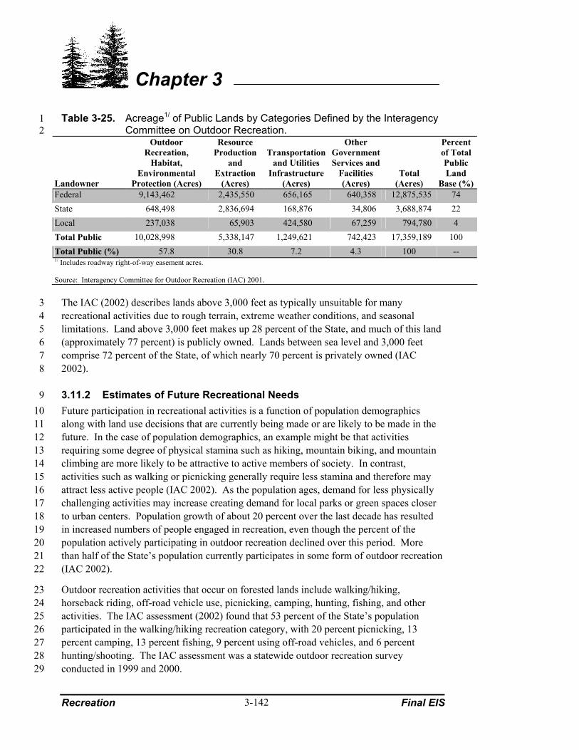
Recreation Final EIS
Chapter 3
3-142
Table 3-25. Acreage1/ of Public Lands by Categories Defined by the Interagency 1 Committee on Outdoor Recreation. 2
Landowner
Outdoor Recreation,
Habitat, Environmental
Protection (Acres)
Resource Production
and Extraction
(Acres)
Transportation and Utilities
Infrastructure (Acres)
Other Government Services and
Facilities (Acres)
Total (Acres)
Percent of Total Public Land
Base (%)Federal 9,143,462 2,435,550 656,165 640,358 12,875,535 74 State 648,498 2,836,694 168,876 34,806 3,688,874 22 Local 237,038 65,903 424,580 67,259 794,780 4 Total Public 10,028,998 5,338,147 1,249,621 742,423 17,359,189 100 Total Public (%) 57.8 30.8 7.2 4.3 100 -- 1/ Includes roadway right-of-way easement acres. Source: Interagency Committee for Outdoor Recreation (IAC) 2001.
The IAC (2002) describes lands above 3,000 feet as typically unsuitable for many 3 recreational activities due to rough terrain, extreme weather conditions, and seasonal 4 limitations. Land above 3,000 feet makes up 28 percent of the State, and much of this land 5 (approximately 77 percent) is publicly owned. Lands between sea level and 3,000 feet 6 comprise 72 percent of the State, of which nearly 70 percent is privately owned (IAC 7 2002). 8
3.11.2 Estimates of Future Recreational Needs 9 Future participation in recreational activities is a function of population demographics 10 along with land use decisions that are currently being made or are likely to be made in the 11 future. In the case of population demographics, an example might be that activities 12 requiring some degree of physical stamina such as hiking, mountain biking, and mountain 13 climbing are more likely to be attractive to active members of society. In contrast, 14 activities such as walking or picnicking generally require less stamina and therefore may 15 attract less active people (IAC 2002). As the population ages, demand for less physically 16 challenging activities may increase creating demand for local parks or green spaces closer 17 to urban centers. Population growth of about 20 percent over the last decade has resulted 18 in increased numbers of people engaged in recreation, even though the percent of the 19 population actively participating in outdoor recreation declined over this period. More 20 than half of the State’s population currently participates in some form of outdoor recreation 21 (IAC 2002). 22
Outdoor recreation activities that occur on forested lands include walking/hiking, 23 horseback riding, off-road vehicle use, picnicking, camping, hunting, fishing, and other 24 activities. The IAC assessment (2002) found that 53 percent of the State’s population 25 participated in the walking/hiking recreation category, with 20 percent picnicking, 13 26 percent camping, 13 percent fishing, 9 percent using off-road vehicles, and 6 percent 27 hunting/shooting. The IAC assessment was a statewide outdoor recreation survey 28 conducted in 1999 and 2000. 29

Final EIS Recreation
Chapter 3
3-143
Participation in all of these activities, with the exception of fishing and hunting/shooting, is 1 projected to increase by 2023. Increases by 2013 are expected to range from 5 to 10 2 percent for camping to 20 percent for picnicking. The numbers of people fishing and 3 hunting/shooting are projected to decrease by 5 percent and 15 percent, respectively, over 4 the same period (IAC 2003). 5
Land use decisions, including the conversion of forestland into uses incompatible with 6 timber production also affect recreational trends. Subsection 3.2 (Land Ownership and 7 Land Use) discusses the rate of land conversion over the past century. Additionally, many 8 cities in the State have designated urban growth areas where it is expected that future land 9 uses will be oriented toward urban development rather than being managed or preserved as 10 forestland. As urban development and forestland conversion continues, there may be a 11 shift in the availability and types of recreational activities. 12
3.11.3 Private Lands and Recreation 13 Currently in Washington State, private landowners play a key role in recreation. Smaller 14 landowners sometimes provide formal facilities, such as campgrounds and golf courses 15 that are available to the public on a fee basis, while some larger and industrial timberland 16 owners operate on a “good neighbor” policy and allow the public access to their lands for 17 general recreational purposes (IAC 2002). 18
In an IAC assessment performed in Washington State in 2002, the recreating public 19 demonstrated concerns regarding increasing needs for better maintenance of public 20 facilities, while local managers of public lands statewide expressed concerns about 21 decreasing funds available for public facilities. As resources for operation and 22 maintenance of recreation facilities on public lands decline, the public may eventually be 23 forced to rely more heavily on undeveloped private lands for recreational needs. 24
3.11.4 Forest Road-related Recreation 25 Existing forest road systems generally receive heavy recreation-related use, providing the 26 public with access to specific recreation areas, such as trailheads, campgrounds, and picnic 27 areas. In addition, a large portion of recreational users of managed forestlands use the road 28 systems as the primary focus of their recreational activity; driving the road systems and 29 occasionally dispersing across the landscape to hunt, bird watch, gather mushrooms or 30 berries, or engage in some other non-facility oriented activity. A recent survey, for 31 example, estimated that approximately 50 percent of back road and “off of road” fuel use 32 in the State of Washington was associated with hunting, driving, sightseeing, camping, and 33 fishing, with the other 50 percent used for off-road motorized activities (off-road vehicles 34 and snowmobiling) and access for non-motorized activities (hiking, mountain biking, 35 cross-county skiing, and equestrian) (Hebert Research, Inc. 2003). 36

Recreation Final EIS
Chapter 3
3-144
This page is intentionally left blank. 1
2

Final EIS Visual Resources
Chapter 3
3-145
3.12 VISUAL RESOURCES 1
3.12.1 Introduction 2 High quality scenery, especially scenery with natural appearing landscapes, is generally 3 regarded as an important resource that enhances peoples’ quality of life, influences the 4 quality of their recreational experiences, and, in some cases, effects the adjacent property 5 values. Forestlands are considered to be an important visual or scenic resource by many 6 Washington State residents and visitors. Approximately 53 percent of the lands in 7 Washington State are forested (23 million out of 43 million acres) (Table 3-2). 8
Table 3-26 presents the percentage of each analysis region that is forested and the 9 percentage of the forestlands that are subject to Washington Forest Practices Rules. The 10 visual resource provided by a forest depends on observer characteristics, as well as the 11 physical properties of the forest landscape. Important observer characteristics include: the 12 amount of concern individual observers have for visual quality, the number of observers, 13 the frequency and duration of their viewing, the context of viewing (e.g., hiking, driving), 14 and attitudes towards visible forest management activities (Bergen et al. 1995; Sheppard 15 1989; Magill 1992). Physical properties of the forest landscape that generally influence the 16 quality of the visual resource provided by forests include: type and density of vegetation, 17 topography, slope and aspect, presence of water, number and type of viewpoints, distance, 18 and weather (Bergen et al. 1995; Shepard 1989). 19
Primary areas where forest-related visual concerns exist include major highway corridors, 20 cities and towns, adjacent housing developments, and trails and other recreation areas. 21 Forested landscapes in these areas are often highly visible to the public and can be 22 managed to reduce the visual impact of harvest and road-building activities. 23
The public’s concern with forestland-related visual resources and quality has increased and 24 continues to increase for a number of reasons. Washington State’s population continues to 25 grow, increasing by approximately 21 percent, or 1 million people, between 1990 and 2000 26 (U.S. Census Bureau 2000). Scenic touring and viewing has continued to increase since it 27 first gained popularity following World War II when more families began to purchase cars 28 and use them for pleasure trips (Dakin 2003; Wilson 1991). Demands for outdoor 29 recreation in Washington State have increased, as shown by visits to State parks, which 30 increased from 12.9 million visits in 1965 to 42.3 million visits in 1997 (Washington DNR 31 1998h). Outdoor recreation takes place on public and private forestland where allowed. 32 Sightseeing was identified as the fifth most popular recreation activity by Washington 33 residents out of 15 recreation categories. Fifty percent of those individuals, who listed 34 sightseeing as one of their recreation activities, choose to sightsee in scenic areas, often 35 forestlands, while the other 50 percent sightsee in other areas such as historical areas 36 (IAC 2002). 37
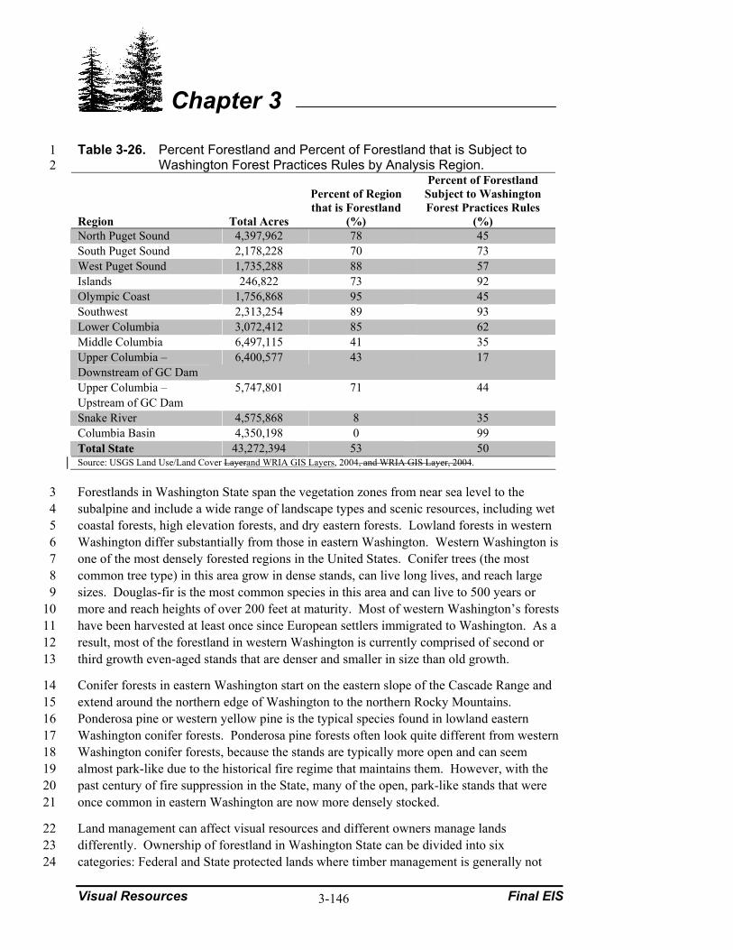
Visual Resources Final EIS
Chapter 3
3-146
Table 3-26. Percent Forestland and Percent of Forestland that is Subject to 1 Washington Forest Practices Rules by Analysis Region. 2
Region Total Acres
Percent of Region that is Forestland
(%)
Percent of Forestland Subject to Washington Forest Practices Rules
(%) North Puget Sound 4,397,962 78 45 South Puget Sound 2,178,228 70 73 West Puget Sound 1,735,288 88 57 Islands 246,822 73 92 Olympic Coast 1,756,868 95 45 Southwest 2,313,254 89 93 Lower Columbia 3,072,412 85 62 Middle Columbia 6,497,115 41 35 Upper Columbia – Downstream of GC Dam
6,400,577 43 17
Upper Columbia – Upstream of GC Dam
5,747,801 71 44
Snake River 4,575,868 8 35 Columbia Basin 4,350,198 0 99 Total State 43,272,394 53 50 Source: USGS Land Use/Land Cover Layerand WRIA GIS Layers, 2004, and WRIA GIS Layer, 2004.
Forestlands in Washington State span the vegetation zones from near sea level to the 3 subalpine and include a wide range of landscape types and scenic resources, including wet 4 coastal forests, high elevation forests, and dry eastern forests. Lowland forests in western 5 Washington differ substantially from those in eastern Washington. Western Washington is 6 one of the most densely forested regions in the United States. Conifer trees (the most 7 common tree type) in this area grow in dense stands, can live long lives, and reach large 8 sizes. Douglas-fir is the most common species in this area and can live to 500 years or 9 more and reach heights of over 200 feet at maturity. Most of western Washington’s forests 10 have been harvested at least once since European settlers immigrated to Washington. As a 11 result, most of the forestland in western Washington is currently comprised of second or 12 third growth even-aged stands that are denser and smaller in size than old growth. 13
Conifer forests in eastern Washington start on the eastern slope of the Cascade Range and 14 extend around the northern edge of Washington to the northern Rocky Mountains. 15 Ponderosa pine or western yellow pine is the typical species found in lowland eastern 16 Washington conifer forests. Ponderosa pine forests often look quite different from western 17 Washington conifer forests, because the stands are typically more open and can seem 18 almost park-like due to the historical fire regime that maintains them. However, with the 19 past century of fire suppression in the State, many of the open, park-like stands that were 20 once common in eastern Washington are now more densely stocked. 21
Land management can affect visual resources and different owners manage lands 22 differently. Ownership of forestland in Washington State can be divided into six 23 categories: Federal and State protected lands where timber management is generally not 24

Final EIS Visual Resources
Chapter 3
3-147
allowed (e.g., wildernesses, parks, and refuges), Federal lands managed under the 1 Northwest Forest Plan, State lands managed for timber under the Washington Forest 2 Practices Rules, tribal forestlands, county and city forestlands, and private forestlands 3 (Table 3-1). Private forestlands may be divided into industrial forestlands where intensive 4 forest practices take place and other private forestlands where forest practices are generally 5 periodic. 6
Federal- and State-protected lands are not managed for timber production and are, 7 therefore, not likely to be affected by Washington Forest Practices Rules. Federal lands 8 managed under the Northwest Forest Plan are managed under an extensive set of scenery 9 management rules (USDA Forest Service and USDI Bureau of Land Management 1994). 10 State lands managed for timber are also managed under policies that require consideration 11 of potential visual impacts, but they permit more extensive visual alteration than the 12 Federal Northwest Forest Plan (USDA Forest Service and USDI Bureau of Land 13 Management 1994). Private, tribal, and other lands can also be managed for timber, often 14 with fewer restrictions on harvest and road building for visual reasons. When these 15 forestlands are converted to other land uses, the visual resource can be substantially 16 impacted (conversion is discussed in subsection 3.2, Land Ownership and Use). 17
3.12.2 Visual Resources and the Current Washington Forest Practices 18 Rules 19
When forests are managed for timber in Washington State, landowners are subject to 20 Washington Forest Practices Rules, which include prescriptions that, although not their 21 primary intent, provide some protection for visual resources during timber harvest. 22 Clearcut harvest areas are prohibited from being larger than 240 acres. Clearcuts must 23 retain at least five uncut trees per acre in western Washington and four uncut trees per acre 24 in eastern Washington for wildlife. Uncut trees are also sometimes required to be left on 25 unstable slopes (WAC 222-10-030 (4)), and landowners are required to leave riparian 26 buffers adjacent to most streams. 27
Riparian buffers requirements, which have existed for nearly two decades, have increased 28 since the current Washington Forest Practices Rules were implemented in April 2000. 29 Under these rules the required widths for buffers adjacent to streams are wider and apply to 30 more streams than was previously required (WAC 222-30). The Washington Forest 31 Practices Rules contribute to the protection of visual resources on State and private 32 forestlands. In addition to these rules, many private forest landowners voluntarily leave 33 additional buffers specifically for visual resource protection. Many Industrial forest 34 landowners use Guidelines For The Design Of Harvest Practices In Visually Sensitive 35 Areas (Bradley 1996) to assist them in planning harvests when they are dealing with 36 visually sensitive landscapes. 37
Practices employed by industrial forest landowners in visually sensitive landscapes may 38 include leaving uncut buffers along major highways, leaving buffers along topographic 39 features to reduce the visual impact of the timber harvest, using selective harvest methods 40 instead of clearcut harvesting, harvesting timber in a way that simulates natural patterns, 41 providing roadside signs that explain the forest practices that have taken place, minimizing 42

Visual Resources Final EIS
Chapter 3
3-148
forest openings next to highways, protecting special vistas with no-harvest areas, and using 1 intensive management to help the harvest area regenerate quickly (Merrill and Ring 1999; 2 Plum Creek 1999; Champion Pacific Timberlands 2000). 3
4

Final EIS Archaeological, Historical, Cultural and Indian Trust Resources
Chapter 3
3-149
3.13 ARCHAEOLOGICAL, HISTORICAL, CULTURAL AND INDIAN 1 TRUST RESOURCES 2
3.13.1 Introduction 3 Cultural resources are districts, sites, buildings, structures, and objects that contain 4 evidence of past human activities or that play an active part in the traditional cultures of the 5 disparate ethnic groups that comprise Washington’s populace. Cultural resources have 6 been recognized by legislative bodies at the Federal and State levels as being important for 7 the education and inspiration of future generations of Americans, whatever their 8 backgrounds. Four categories of cultural resources are recognized and discussed here and 9 in the environmental effects section, as defined below. 10
Archaeological Resources—the physical residues of past human activity. Archaeological 11 resources provide evidence of the cultural continuum of people occurring across time and 12 space throughout the diverse landscapes of Washington. Examples of archaeological 13 resources include shell middens, scatters of stone chips (lithic scatters), rock art, talus slope 14 gravesites, and culturally modified trees. 15
Historic Sites—locations where Native or non-Native events and activities have taken 16 place since contact with Euro-Americans. Historic sites often, but not always, have written 17 records that document the events and activities that occurred at a particular location. 18 Examples of historic sites include homesteads, forts, lumber mills, cabins, mine shafts, and 19 old logging or mining equipment. 20
Traditional Places—landscapes, resource gathering areas, sacred sites, and legendary 21 areas that are identified (often with traditional names) by Indian Tribes in the State of 22 Washington as being important for the maintenance and perpetuation of their traditional 23 values and practices. These landscapes, places, and objects provide subsistence and 24 spiritual relationships, as well as stability and meaning to community ceremonies, customs, 25 and beliefs. Examples of traditional places include sacred ceremonial sites, groves used for 26 gathering edible/medicinal plants, and sources of materials used for traditional tools and 27 arts. 28
Traditional Materials—the resources used by Native peoples to sustain their culture. 29 Traditional materials come from the broad variety of plants, animals, and minerals that are 30 indigenous to this region’s native landscapes. Traditional and current cultural values for 31 plants include their use as medicines, foods, tools, textiles, building materials, carvings, 32 and sacred objects. Examples of traditional materials (such as some of the plants utilized 33 by Tribes) include bear grass, tule, and cedar and birch trees. 34
3.13.2 Archaeological Overview 35 Lands lying west and east of the Cascade Range have been ecologically distinct for most of 36 the postglacial period as well as being geographically separated by the mountain range. 37 Consequently, cultural developments and archaeological site distributions are also distinct. 38

Archaeological, Historical, Final EIS Cultural and Indian Trust Resources
Chapter 3
3-150
3.13.2.1 Western Washington 1 Despite nearly a century of scientific research in the region, the archaeology of western 2 Washington is not well understood. Most of what is known comes from low elevation 3 lands that are now largely under agricultural and residential development. The foothills 4 and lower mountain settings, where most of the region’s productive forests can be found, 5 have received relatively little attention from archaeologists. What is known about the 6 prehistoric archaeology of the region is, consequently, biased toward the lowlands, 7 particularly coastlines. Much of the property managed by the State and the majority of 8 privately owned forestlands has not been intensively surveyed for archaeological resources; 9 the same is true for nearby lands of the National Forests. Most archaeological sites in these 10 forests have been found along streams or on high ridges, but this may be due in part to a 11 tendency for land managers to survey what they consider high probability areas more 12 intensively than lower probability slopes. What is currently known about the archaeology 13 of western Washington is summarized below. 14
The first human occupation of Washington State may date back about 14,000 years1 to the 15 Manis Mastodon site at Sequim. Artifacts of the 13,000- to 13,500-year-old Clovis culture, 16 which is thought to have been focused on big game hunting, have been found on the 17 ground surface in such places as Thurston County and Whidbey Island, but no campsite of 18 this culture has yet been found in Washington. 19
The post-Clovis prehistory of western Washington has been divided into three periods, 20 designated as Early, Middle, and Late. The Early Period, which lasted from approximately 21 12,000 to 7,000 years ago, includes the Proto-Western and Old Cordilleran Traditions 22 (Matson and Copeland 1995). Sites left by these traditions typically occur on high marine 23 and river terraces, sometimes at a significant distance from modern water courses, and 24 consist of concentrations of cobble cores, flakes, large, ovate knives, and broad-stemmed 25 and leaf-shaped projectile points (Wessen 1990). In some areas, sites of this period have 26 also been documented along mountain streams in open sites, rockshelters, and caves 27 (Wessen and Stilson 1986; Lewarch and Benson 1989). Because of an apparent inland 28 focus, the people of this era are thought to have been more oriented to land animal hunting 29 and less to marine and fish resources. 30
The Middle Period, lasting from 7,000 to 3,500 years ago sees a continuation of the Old 31 Cordilleran Tradition until around 4,500 years ago, but few sites can be attributed to this 32 time interval (Morgan 1999). The focus of subsistence activity after 4,500 years ago seems 33 to have changed from terrestrial to marine resources and most sites appear along the coasts 34 or major river systems. There is little evidence of activity in the higher mountains. Tools 35 are more complex, including tools and ornaments of bone and antler along with chipped 36 stone (e.g., Larson and Lewarch 1995). 37
The concentration on marine resources intensified during the Late Period (3,500 to 150 38 years ago), and the number and diversity of sites increased markedly. People maintained 39
1 Dates given here are in calendric years, based on approximate calibration of radiocarbon ages.

Final EIS Archaeological, Historical, Cultural and Indian Trust Resources
Chapter 3
3-151
permanent villages on the coast and along the lower reaches of inland rivers, which they 1 used as home bases and storage warehouses. Huge shell middens built up at some villages 2 and at the best clam beaches. Cemeteries and petroglyph sites are often associated with 3 village and midden sites and fishing camps and occur occasionally in higher montane 4 settings. Blazed cedars, stripped of bark for basketry or with planks removed from their 5 living trunks, can still be found throughout the lowlands. Small open camps, left by 6 hunters, fishers, berry pickers (Mack and McClure 2002), and traders have been found 7 from the lowlands well into the subalpine zone of the mountains, but usually remain close 8 to larger, permanent sources of water. They typically are concentrated along trade routes. 9
Archaeological sites in western Washington consist of the remains of villages and their 10 associated cemeteries and petroglyph sites, saltwater shell middens, temporary camps 11 consisting of stone flaking debris (lithic scatters), berry processing camps, rockshelters and 12 caves, and stone quarries. With the exception of quarrying areas, berry processing 13 localities and some caves, rockshelters, and petroglyphs, most archaeological sites in 14 western Washington occur close to streams and shorelines (Nelson 1990). 15
A type of archaeological site that has recently been recognized is the culturally-modified 16 tree. These are typically living cedar trees that have had bark stripped from one or more 17 sides of the tree for use in making baskets or clothing. Culturally-modified trees are 18 expected in stands of old-growth cedar that predate intensive Euro-American settlement 19 (Larson 1998; Gunther 1973). 20
3.13.2.2 Eastern Washington 21 Lands east of the Cascade Range tend to be drier and more open, except at higher 22 elevations, and the archaeology of the region is proportionately better known than the 23 western region. The prehistory of this region begins much the same as that of western 24 Washington, with scattered manifestations of the Clovis Culture. Post-Clovis archaeology 25 is again divided into Early, Middle and Late, but the beginning and ending points of these 26 periods differ from those of western Washington (Ames et al. 1998; Chatters and Pokotylo 27 1998). 28
The Early Period, from 11,000 to 8,000 years ago, is characterized by large, stemmed 29 projectile points, ovate knives, barbed harpoons, grooved net weights, and a stone tool 30 technology reminiscent of the upper Paleolithic technologies of Eurasia. Few sites of this 31 time period have been found, most of them consisting of small campsites along rivers and 32 streams of the non-forested lowlands. A few sites of this period have been reported from 33 the Blue Mountains, but none are yet known from the Cascades. 34
During the Middle Period, 8,000 to 5,000 years ago, the region was occupied by a variant 35 of the Old Cordilleran Culture, known locally as Cascade. Cascade sites are ubiquitous 36 along the Snake and Columbia Rivers, and their larger tributaries and occasionally occur as 37 open camps and in rockshelters in all mountain ranges. There is some indication that 38 quarries in the eastern Cascade Range were in use at this time. Artifacts of this period 39 resemble comparable assemblages from western Washington, consisting of cobble tools, 40
Archaeological, Historical, Final EIS Cultural and Indian Trust Resources
Chapter 3
3-152
cobble flakes, leaf-shaped projectile points and knives, simple scraping tools, occasional 1 microblades, and little else (Ames et al. 1998). 2
During the Late Period, which is comprised of a sequence of distinct cultural adaptations, 3 people had begun to settle in pithouse villages along major streams. They followed a 4 seasonal subsistence routine that included early springtime camps away from the villages 5 but still in riverine settings, root gathering camps near springs in foothills and at mountain 6 meadows, berry picking camps in the subalpine forests, and hunting camps throughout the 7 landscape in caves, near springs, and along water courses. Special purpose sites are 8 common from this Period and include cemeteries near villages, isolated graves and rock art 9 panels in many settings, quarrying areas, spirit quest cairns and game drives on ridgetops, 10 hunting blinds and storage pits in talus slopes, storage caves, and culturally modified trees. 11 In eastern Washington forests, culturally modified trees may include cedars stripped of 12 bark for making baskets or pines stripped of edible cambium (Hunn et al. 1998). 13
There is an even more marked tendency in this region for sites to concentrate near springs 14 and streams. Cemeteries, villages, and most camps are rarely far from water, although 15 special purpose sites may occur at considerable distance (Galm et al. 1981). 16
3.13.3 Cultural and Trust Resources of Native American Tribes 17 Historic native cultures of the region can generally be seen as a continuation of the 18 lifeways indicated by Late Period archaeological sites. The region’s peoples belonged to 19 five linguistic groups: Wakashan, Salishan, Chimakuan, Chinookan, and Sahaptian. 20 Wakashan, Chinookan, Chimakuan, and most Salishan peoples were marine oriented, 21 occupying villages on the major rivers or saltwater shorelines of western Washington and 22 focusing on shellfish, and salmon and/or saltwater fish for their subsistence. These peoples 23 abandoned their villages in summer, moving among fishing sites, and hunting, root 24 gathering, and berrying camps in mountains and prairies (Haeberlin and Gunther 1930; 25 Silverstein 1990). The Salishan Snoqualmie and the Sahaptian-speaking Klikitat differed 26 from other western Washington Tribes, spending most of their time in foothill and 27 mountain settings, where they emphasized hunting, berrying, and root gathering, and 28 served as intermediaries in the transmontane trade (Suttles and Lane 1990; Walker 1998). 29
All eastern Washington Tribes belong either to the Salishan or Sahaptian language 30 families. Members of these groups focused on salmon fishing, root and berry gathering, 31 and big game hunting for their subsistence in varying proportion, depending on the 32 resources of their respective territories. In a continuation with the Late Period of 33 prehistory, they occupied villages of pithouses or mat lodges in winter along major stream 34 courses and moved among a series of smaller camps or multi-band conclaves as the year 35 progressed. They were linked to the peoples of the western flank of the Cascades and 36 Lower Columbia River through trade and intermarriage (Miller 1998; Schuster 1998). 37
Today, 29 federally recognized Tribes reside in Washington (Table 3-27) and over a dozen 38 Tribes that once lived in what is now Washington State, reside in adjacent states and 39 Canada. The Tribes that entered into treaties with the United States in 1855 (i.e., all the 40

Final EIS Archaeological, Historical, Cultural and Indian Trust Resources
Chapter 3
3-153
Table 3-27. Federally-Recognized Tribes of Washington and Adjacent States 1 with Cultural Interests in Washington Forests. 2
Region Tribes Eastern Washington Coeur D’Alene1, Colville, Nez Perce1/, Spokane, Pend d’Oreille,
Umatilla1, Yakama Western Washington Shoalwater Bay Chinook, Chehalis, Cowlitz, Hoh, Lummi, Makah,
Muckleshoot, Nisqually, Nooksack, Puyallup, Quileute, Quinault, Sauk-Suiattle, Upper Skagit, Lower Elwha, Jamestown, Port Gamble, S’Klallum, Skokomish, Snoqualmie, Squaxin Island, Stillaguamish, Suquamish, Swinomish, Tulalip
1/ With reservations outside Washington.
Tribes in Table 3-27 except the Colville, Chehalis, Cowlitz, Shoalwater Chinook, Spokane, 3 and Coeur D’Alene) all retained the right to certain resources on ceded territories. All 4 treaties reserve the right to fish in usual and accustomed grounds and places in common 5 with other citizens, and to hunt and gather roots and berries on open and unclaimed land. 6
The right to fish carries with it a trust responsibility on the part of the Federal government 7 to help ensure the continued productivity of the fishery. 8
Forests provide raw materials for Washington’s Tribes (e.g., bark and grasses for baskets 9 and mats, wood for carvings, and medicinal plants) as well as subsistence resources 10 (Gunther 1973). While each tribal group is different in the plants and animals that it 11 considers culturally important, and while many of the medicinal and ceremonial species are 12 kept secret for religious or other cultural reasons, some plants and animals that have 13 importance across many groups are listed in Table 3-28. Salmon, deer, elk, cedar, 14 beargrass, and huckleberries are the most prominent among these resources. 15
Of the culturally important resources listed in Table 3-28, most occur or are most abundant 16 in the water (fishes, shellfish, some mammals), streamside wetlands (tule, cattail), 17 meadows (camas, nettle, many berries and roots), or early seral stages of forests (most 18 berries, beargrass, nettle, bracken, alder, big game). Some species, however, occur or are 19 most useful when found in old-growth stands (cedar, spruce, tree lichen) (Turner 1978; 20 Gunther 1973). 21
Mature forests also provide solitude that is necessary for individuals’ quests for personal 22 spirit guidance, and for the observance of spirit dances among some Salishan groups 23 (Hajda 1990; Kew 1990; Suttles and Lane 1990). The quest for spiritual guidance begins 24 before puberty and continues throughout a person’s life (Haeberlin and Gunther 1930; 25 Walker 1998). Forestlands also contain many traditional places, which can take many 26 forms, from rock outcroppings or caves to cedar groves or camas meadows. Some Tribes 27 have worked with land managers to identify sacred places and stands of culturally 28 important plants (e.g., Blukis-Onat and Hollenbeck 1981), while others prefer to keep such 29 locations secret. 30
31

Archaeological, Historical, Final EIS Cultural and Indian Trust Resources
Chapter 3
3-154
Table 3-28. Culturally Important Plant and Animal Resources for Native 1 American Tribes in Washington. 2
Resources Western Washington1/ Eastern Washington2/ Fishes3/ Chinook, coho, pink, chum, and
sockeye salmon, steelhead, cutthroat trout, dolly varden trout, smelt
Chinook, coho, and sockeye salmon, steelhead, bull trout, cutthroat trout, lamprey, suckers, mountain whitefish
Shellfish3/ Freshwater mussels
Mammals4/ Blacktail deer, elk, bear, otter, beaver
Deer, elk, blackbear, otter
Berries, Roots, and Other Foods Huckleberries, blueberries, trailing blackberry, black cap, salmonberry, thimbleberry, salal berry, serviceberry, soapberry; wild carrot, wapato, camas, bracken root, sand verbena, thistle root, surf grass, buttercup, clover roots; cow parsnip
Blue huckleberry, serviceberry, chokecherry, currant, blackberry; camas, wild carrot, chocolate lily; tree lichen; pine cambium; wild celery
Raw Materials Yew, alder, and cedar wood, spruce root, cedar, hemlock, and willow bark, beargrass, nettle, cattail, and tule
Cedar bark, wood and boughs, beargrass, tule
1/ Renker and Gunther 1990; Gunther 19451973; Powell 1990; Suttles and Lane 1990; Silverstein 1990. 2/ Schuster 1998; Ross 1998; Kennedy and Bouchard 1998; Stern 1998; Walker 1998. 3/ Freshwater or anadromous, only. 4/ Terrestrial only.
3.13.4 Overview of Regional History 3 Washington’s coastline was first charted and described by English and American Explorers 4 in the last decades of the eighteenth century. Fur traders, primarily associated with Forts 5 Vancouver, Nisqually, Walla Walla, Okanagan, and Spokane, traveled into the interior in 6 the first half of the nineteenth century. Except for the increasing presence of beads, metal, 7 and other trade goods among the local Indian Tribes, they left few traces outside their fort 8 compounds. By the 1830s, the Hudson’s Bay Company had expanded into agricultural 9 production, maintaining large farms in the lowlands around Forts Vancouver and Nisqually 10 and in the lower Cowlitz River Valley. Missionaries soon followed the fur traders, setting 11 up missions in the Yakima and Walla Walla Valleys during the 1840s. Settlers, some 12 drawn by the promise of farmland, but most coming to exploit the region’s timber and 13 mineral wealth began flowing into the Puget Lowlands and Portland Basin by the late 14 1840s and into eastern Washington after the 1855 signing of treaties with the region’s 15 Indian Tribes. The farmers needed water and, like their Native predecessors, settled first in 16 valley bottoms and along small stream courses, particularly in the drier eastern part of the 17 state. Loggers and fishermen built along the coasts and exploited lowland timber from the 18 onset of settlement. By the latter part of the nineteenth century, Euro-Americans also 19 began to exploit the timber and mineral resources of the non-arable mountains in western 20 Washington, and began to mine, log, and graze stock in the open forests of eastern 21
Final EIS Archaeological, Historical, Cultural and Indian Trust Resources
Chapter 3
3-155
Washington (Avery 1965). Railroads and haul roads were built into and across the 1 Cascades for hauling timber, coal, stock, and produce to markets and to connect 2 Washington with the rest of the United States. 3
Past farming and stock raising activities are marked by buildings, water control structures, 4 fences, and stock camps. Mining has left its traces throughout the uplands of Washington. 5 Coal mining is marked by large, open pit mines and haul roads, whereas traces of past gold 6 mining occur as placer tailings, mining prospects, mine shafts, and miners’ camps. Sites 7 associated with logging include skid roads, railroad grades and tracks, trestles, construction 8 and logging camps, stumps cut with springboard notches, and a variety of equipment. 9
3.13.5 Washington State Protective Structure 10 Washington State makes use of many venues for protection and preservation of 11 archaeological, historical, and cultural resources, including the Office of Archaeology and 12 Historic Preservation, protective statutes in the RCW, and protective regulations in the 13 WAC. 14
The Office of Archaeology and Historic Preservation provides expertise, service, and 15 training for the protection and preservation of Washington’s historic places. The office 16 manages programs to aid historic property owners, community leaders, and preservation 17 advocates. A key role of the Office of Archaeology and Historic Preservation is the 18 identification, evaluation, and protection of significant properties worthy of preservation 19 (Washington State Community, Trade, and Economic Development 1996). The office is a 20 center for data collection and administers the National Register of Historic Places and the 21 Washington Heritage Register. The Office of Archaeology and Historic Preservation is a 22 part of the Washington State Department of Community, Trade, and Economic 23 Development. The Director of this department, or their designee, is a member of the 24 Forest Practices Board, the promulgating agency for Washington Forest Practices Rules. 25
Various state agencies interface with archaeological, historical, and cultural resources. The 26 Washington Department of Transportation has a Cultural Resources Program that keeps the 27 public, including Washington Tribes, informed about Department of Transportation 28 projects and actively seeks the public’s input on concerns about project impacts on 29 archaeological, historical, or cultural resources (Personal Communication, Sandie Turner, 30 Transportation Planning Specialist, Department of Transportation, August 19, 2004). 31 Washington State Parks and Recreation protects many archaeological, historical, and 32 cultural resources on their properties. Washington DNR interfaces with cultural resources 33 in both the regulatory arena and the land management arena. 34
The Washington DNR Forest Practices Regulatory Program regulates forest practices in 35 the state including forest practices affecting archaeological, historical, and cultural 36 resources on both private and State land (WAC 222). In addition to the forest practices 37 regulations, the Cultural Resource Protection and Management Plan, written and agreed to 38 by TFW participants on July 3, 2003, provides a process to enhance protection of cultural 39 and archeologicalarchaeological sites on managed forestlands (Timber, Fish, and Wildlife 40 Cultural Resources Committee 2003). 41

Archaeological, Historical, Final EIS Cultural and Indian Trust Resources
Chapter 3
3-156
Washington DNR State Lands program manages 2.1 million acres of forestland in the State 1 where archaeological, historical, and cultural resources may be found. Washington DNR 2 has a tribal Relations Manager who is a liaison between Washington DNR State Lands and 3 Washington Tribes and is working on strengthening and focusing Washington DNR State 4 Lands’ Cultural Resources program (Personal Communication, Joseph Davis, Washington 5 DNR, August 18, 2004). The Commissioner of Public Lands, the head of Washington 6 DNR, recently reaffirmed Washington DNR’s commitment of collaborative tribal 7 relationships in a Commissioner’s Order, stating that the Department will “actively work 8 with Tribes to encourage understanding and the cooperative pursuit of common objectives” 9 (Department of Natural Resources, Commissioner’s Order, April, 26, 2004a.) 10
The Department of Transportation, Washington State Parks and Recreation, and the Office 11 of Archaeology and Historic Preservation offer a weeklong semi-annual training course on 12 cultural resources. The course provides information for recognition and protection of 13 resources as well as information on State agency legal obligations centered on 14 archaeological, historical, and cultural resources. The course includes site visits to help 15 students learn how to recognize an archaeological, historical, or cultural resource. 16

Final EIS Social and Economic Environment
Chapter 3
3-157
3.14 SOCIAL AND ECONOMIC ENVIRONMENT 1
3.14.1 Introduction 2 This section presents a general overview of the social and economic conditions of 3 Washington State, and provides a baseline that the potential effects of the alternatives may 4 be measured against. The discussion is organized into three sections that address 5 population, employment and the economy, and environmental justice. 6
3.14.2 Population 7 The total population of Washington State was approximately 5.9 million in 2000, an 8 increase of 21 percent, or approximately 1 million people, since 1990. All Washington 9 counties experienced population growth during the 1990s, with increases ranging from 10 1 percent in Columbia County to 45 percent in Clark County. Net in-migration accounted 11 for 63 percent of statewide population growth over this period and contributed to 12 population increases in all Washington counties, with the exception of Whitman County, 13 where net out-migration accounted for approximately -1 percent of population change. 14 The majority of Washington counties also experienced natural increase (more births than 15 deaths) over this period. There were, however, some exceptions, including Columbia, 16 Garfield, Pacific, Wahkiakum, Clallam, Jefferson, and Lincoln Counties, where there were 17 more deaths than births (Washington Office of Financial Management 2004). 18
The statewide population density in 2000 was 88.6 persons per square mile compared to a 19 national average of 79.6 percent. Population density varies considerably by county, 20 ranging from 4.7 persons per square mile in Columbia County in southeast Washington to 21 817 persons per square mile in King County. Population densities were, not surprisingly, 22 highest in those counties that include major urban areas: the Puget Sound area (King, 23 Kitsap, Pierce, Snohomish, and Thurston Counties), Vancouver (Clark County), and 24 Spokane (Spokane County). Population densities in counties elsewhere in the State were 25 less than 100 persons per square mile and many counties, particularly those located in the 26 northeast part of the State, had population densities below 20 persons per square mile 27 (Washington Office of Financial Management 2004). 28
Population projections developed by the Washington Office of Financial Management in 29 2002 anticipate continued growth in the State, with the total State population projected to 30 reach 7.5 million by 2020. Population is projected to increase in all counties over this 31 period, with increases ranging from 2 percent in Columbia County to 50 percent in 32 Thurston County (Washington Office of Financial Management 2002a). 33
3.14.2.1 Race and Ethnicity 34 Approximately 85 percent of Washington’s population identified as white in the 2000 35 Census, compared to 75 percent nationwide. Compared to the national average, Black or 36 African American persons and persons of Hispanic or Latino origin were relatively under-37 represented, comprising smaller shares of the State population than the national average. 38 Asian and American Indian persons were, by the same measure, relatively over 39
Social and Economic Environment Final EIS
Chapter 3
3-158
represented, comprising slightly larger shares of the State population than the national 1 average (U.S. Census Bureau 2000). 2
The percentage of the population identifying as white varied by county, ranging from 3 approximately 62 percent in Franklin County to approximately 97 percent in Garfield 4 County. Persons of Hispanic or Latino origin comprised relatively large shares of the 5 population in Adams (40 percent), Franklin (39 percent), Yakima (28 percent), and Grant 6 (23 percent) Counties. American Indians made up relatively large shares of the population 7 in Ferry (18 percent), Okanogan (12 percent), and Yakima (4.5 percent) Counties 8 (Washington Office of Financial Management 2002b). 9
3.14.3 Employment and the Economy 10 This section provides a general overview of employment and the economy in Washington 11 State. The section discusses two summary measures developed by Federal and State 12 agencies—socioeconomic resiliency and the distressed areas index. It also addresses 13 overall employment trends and employment in the lumber and wood products, commercial 14 fishing, and recreation and tourism industries. 15
3.14.3.1 Socioeconomic Resiliency 16 Socioeconomic resiliency refers to the ability of an area’s population and economy (e.g., 17 community, county, or region) to adapt to economic changes or shocks. Resiliency is 18 generally related to diversity, with areas or socioeconomic systems with higher diversity 19 less affected by a change in the system, such as a change in timber harvest or grazing 20 opportunities. A high degree of resiliency implies that an area or socioeconomic system 21 adapts quickly to economic fluctuations or changes, such as specific firms or business 22 sectors experiencing downturns, with unemployment rates rising only briefly until 23 displaced individuals find other employment. Areas or socioeconomic systems with low 24 resiliency may, on the other hand, experience long-term negative impacts, with 25 unemployment or out-migration rates remaining high for several years. 26
A recent study prepared for Washington DNR assessed the socioeconomic resiliency of 27 Washington counties employing the methodology used to develop measures of 28 socioeconomic diversity for the Interior Columbia Basin Ecosystem Management Project 29 (ICBEMP) (Daniels 2003; Horne and Haynes 1999). The objective of the Washington 30 DNR study was to identify those counties where changes in timber harvest on State lands 31 may have disproportionate negative effects on the well being of county residents. Part of 32 this analysis involved identifying counties of concern, which were defined as those 33 counties with low socioeconomic resiliency and high forest dependency. A socioeconomic 34 resiliency index was developed based on a composite of three related factors: lifestyle 35 diversity, economic diversity, and population density. Forest dependence was identified 36 based on the percent of total county area classified as forestland. Ferry, Pend Oreille, 37 Pacific, Skamania, Stevens, and Wahkiakum Counties all had low socioeconomic 38 resiliency and high forest dependency and were identified as counties of concern. Adams, 39 Okanogan, Klickitat, Columbia, Garfield, and Lincoln Counties also had low 40 socioeconomic resilience, but had low or medium forest dependence ratings (Daniels 41 2003). 42

Final EIS Social and Economic Environment
Chapter 3
3-159
3.14.3.2 Distressed Areas Index 1 The Washington Employment Security Department identifies distressed counties using 3-2 year average unemployment rates. A county is considered distressed if the average 3 unemployment rate is 120 percent or greater than the average statewide unemployment rate 4 (Washington State Employment Security Department 2003). Nineteen counties were 5 identified as distressed areas in 2003 (Table 3-29). 6
Table 3-29. State of Washington Distressed Counties, 2003. 7
State/County 3-Year Average
Unemployment Rate1/ County 3-Year Average
Unemployment Rate1/
Washington State 6.3 Grays Harbor County 9.9 Adams County 10.3 Klickitat County 13.4 Chelan County 8.8 Lewis County 9.1 Clallam County 7.6 Mason County 7.7 Columbia County 11.1 Okanogan County 10.8 Cowlitz County 9.4 Pacific County 8.6 Douglas County 8 Pend Oreille County 9.5 Ferry County 13.2 Skamania County 10.5 Franklin County 9.1 Stevens County 10.1 Grant County 9.9 Yakima County 10.7 1/ The 3-year averages are for January 2000 through December 2002. Source: Washington State Employment Security Department 2003.
3.14.3.3 Employment 8 Employment is summarized by sector for Washington State in Table 3-30 for 1990 and 9 2000. Overall Washington State employment increased by 24 percent or 688,915 jobs 10 between 1990 and 2000, with the largest absolute gains occurring in the services (+325,865 11 jobs), retail trade (+125,545 jobs), and State and local government (+85,630 jobs) sectors. 12 Sectors with relatively large increases included services and also the agricultural services, 13 forestry, fishing, and other sectors. The agricultural services and forestry subsectors, also 14 shown in Table 3-30, experienced relatively large employment increases, while the fishing 15 subsector experienced large relative and absolute job loss over this period (U.S. Bureau of 16 Economic Analysis 2004a). 17
The largest absolute job loss occurred in the manufacturing sector (-17,577 jobs), with job 18 loss in the lumber and wood products accounting for approximately 47 percent of this 19 decline. Job loss also occurred in the Federal government sector, with a net loss of 4,610 20 jobs in the civilian sector, and a further net loss of 8,896 jobs in the military (Table 3-30) 21 (U.S. Bureau of Economic Analysis 2004a). 22
The following sections discuss lumber and wood products, commercial fishing, and 23 recreation and tourism. 24
Social and Economic Environment Final EIS
Chapter 3
3-160
Table 3-30. Washington Employment by Sector, 1990 and 2000. 1 1990 2000 1990-2000
Jobs Percent of Total (%) Jobs
Percent of Total (%)
Absolute Change
Percent Change
(%) TOTAL EMPLOYMENT1/ 2,864,111 100 3,553,026 100 688,915 24 By Type Wage and Salary Employment 2,371,705 83 2,940,967 83 569,262 24 Proprietors Employment 492,406 17 612,059 17 119,653 24 By Industry Farm Employment 81,399 3 80,004 2 -1,395 -2 Nonfarm Employment 2,782,712 97 3,473,022 98 690,310 25
Agricultural Services, Forestry, Fishing, and Other
49,242 2 63,384 2 14,142 29
Agricultural Services2/ 32,777 1 48,273 1 15,496 47 Forestry2/ 4,075 0 5,693 0 1,618 40 Fishing2/ 12,390 0 9,418 0 -2,972 -24 Mining 5,637 0 5,411 0 -226 -4 Manufacturing 388,748 14 371,171 10 -17,577 -5 Lumber and Wood Products2/ 45,664 2 37,460 1 -8,204 -18 Transportation and Public Utilities 128,055 4 168,164 5 40,109 31 Wholesale Trade 141,561 5 168,279 5 26,718 19 Retail Trade 468,693 16 594,238 17 125,545 27 Finance, Insurance, and Real Estate 218,487 8 267,150 8 48,663 22 Services3/ 747,216 26 1,073,081 30 325,865 44 Government and Government Enterprises
475,689 17 547,813 15 72,124 15
Federal, Civilian 73,745 3 69,135 2 -4,610 -6 Military 81,702 3 72,806 2 -8,896 -11 State and Local 320,242 11 405,872 11 85,630 27 1/ Total employment includes self-employed individuals. Employment data are by place of work, not place of residence and, therefore,
include people who work in the area but do not live there. Employment is measured as the average annual number of jobs, both full- and part-time, with each job that a person holds counted at full weight.
2/ Agricultural Services, Forestry, and Fishing are subcategories of the Agricultural Services, Forestry, Fishing and Other Standard Industrial Classification (SIC) division. Lumber and Wood Products is a subcategory of the Manufacturing SIC division.
3/ Examples include hotels/motels, business services, automotive repair and other services, amusement and recreation services, health services, legal services, educational services, social services, engineering and management services, and accounting services.
Source: U.S. Bureau of Economic Analysis 2004a.
Lumber and Wood Products 2 Statewide, a total of 37,460 people were directly employed in the lumber and wood 3 products industry in 2000, approximately 8,200 or 18 percent fewer than were employed in 4 this sector in 1990 (Table 3-30). Timber harvest results in direct employment in the 5 logging and lumber and wood products sectors. It also generates indirect and induced 6 employment. Indirect employment includes jobs associated with industries that supply 7 inputs to the harvesting and processing sector. Induced employment includes jobs 8 associated with spending in the economy from the salaries created by direct and indirect 9 effects. 10

Final EIS Social and Economic Environment
Chapter 3
3-161
Direct employment in the lumber and wood products sector accounted for about 1 percent 1 of total employment statewide, ranging from no covered employment in a number of 2 counties (e.g., Adams, Garfield, and Grant Counties) to 10 or more percent of total covered 3 employment in Mason (10 percent), Stevens (12 percent), and Wahkiakum (25 percent) 4 Counties.1 Viewed in absolute terms, the counties with the largest number of covered jobs 5 in this sector in 2001 were King (5,500 jobs), Pierce (3,500 jobs), and Snohomish (3,000 6 jobs), which together accounted for approximately 41 percent of covered employment in 7 the lumber and wood products sector. Lewis and Grays Harbor Counties followed with 8 approximately 2,100 lumber and wood products jobs each (Washington State Employment 9 Security Department 2004). Covered employment and wage data indicate that the average 10 wage in the lumber and wood products sector in Washington State was approximately 11 $39,700 in 2001 (Washington State Employment Security Department 2004). 12
Washington State was the second largest softwood lumber producer in the United States in 13 2001. Lumber production fluctuated during the 1990s, ranging from 3,820 million board 14 feet in 1991 to 4,384 million board feet in 2000. A total of 4,257 million board feet were 15 produced in 2001 (Warren 2003). 16
Washington timber harvest levels have shown an overall pattern of decline since 1990 17 (Figure 3-10). Harvest levels fluctuated during the 1990s, but ranged from a peak of 5,850 18 million board feet in 1990 to a low of 3,582 million board feet in 2002. Harvest declined 19 for all ownerships over this period, with the exception of tribal harvests, which increased 20 from 182 million board feet in 1990 to 319 million board feet in 2002. Harvest on lands 21 owned by large private (non-industrial) landowners was higher in 2002 than during most of 22 the preceding decade (Figure 3-10). The largest relative decline in harvest occurred on 23 Federal lands with harvest levels decreasing by 90 percent, from 833 million board feet in 24 1990 to just 85 million board feet in 2002. Statewide, private lands accounted for the 25 majority of harvest in 2002, with forest industry lands providing 36 percent of total harvest 26 and large private and small private lands accounting for 27 percent and 11 percent, 27 respectively (Washington DNR 2004b). 28
Counties in western Washington accounted for approximately 75 percent of total harvest in 29 2002 and the majority of harvest on forest industry, private large, private small, and State 30 lands (Table 3-31). This pattern was, however, reversed for tribal and Federal lands with 31
1 Covered employment includes workers covered by State unemployment insurance laws and Federal
workers covered by the Unemployment Compensation for Federal Employees Program. Self-employed persons are not included in covered employment data. This differs from the data summarized in Table 3-29, which include both covered employment and self-employed persons. Covered employment data tend to underestimate total employment in the logging, commercial fishing, and recreation and tourism sectors because people who work in these industries are often self-employed.

Social and Economic Environment Final EIS
Chapter 3
3-162
1
Figure 3-10. Washington Timber Harvest by Owner, 1990 to 2002. 2
Notes: 3 MMBF = million board feet 4 Private Large—Non-industrial companies and individuals not operating wood-using plants but with statewide 5 holdings totaling more than 1,000 acres. 6 Private Small—Non-industrial companies and individuals not operating wood-using plants and with statewide 7 holdings totaling less than 1,000 acres. 8 Data for the Other Non-Federal category are not shown in this figure. Statewide harvest from Other Non-9 Federal lands accounted for 26 million board feet in 2001. 10 Source: Washington DNR Washington Timber Harvest, annual reports 1990 to 2002. 11 12
Table 3-31. Timber Harvest by Ownership and Location, 2001. 13
Tribal Forest
Industry Private Large
Private Small State Federal
Other Non-Federal Total
Harvest (MMBF) Eastside 292 163 172 113 59 66 14 878 Westside 27 1,142 795 297 398 19 26 2,704 Total 319 1,304 967 410 457 85 40 3,582
Percent of Total by Ownership Eastside 92 12 18 28 13 78 34 25 Westside 8 88 82 72 87 22 66 75 Total 100 100 100 100 100 100 100 100 MMBF = million board feet Private Large—Non-industrial companies and individuals not operating wood-using plants but with statewide holdings totaling more than 1,000 acres. Private Small—Non-industrial companies and individuals not operating wood-using plants with statewide holdings totaling less than 1,000 acres. Source: Washington DNR 2004b.
0
5 0 0
1 ,0 0 0
1 ,5 0 0
2 ,0 0 0
2 ,5 0 0
3 ,0 0 0
1 9 9 0 1 9 9 1 1 9 9 2 1 9 9 3 1 9 9 4 1 9 9 5 1 9 9 6 1 9 9 7 1 9 9 8 1 9 9 9 2 0 0 0 2 0 0 1 2 0 0 2
MM
BF
T r ib a lF o re s t In d u s t r yP r iv a te L a rg eP r iv a te S m a llS ta teF e d e ra l
Final EIS Social and Economic Environment
Chapter 3
3-163
counties in eastern Washington accounting for the majority of timber harvest on these land 1 ownerships (Washington DNR 2004b). 2
Commercial Fishing 3 The commercial fishing industry accounted for 9,418 jobs in Washington State in 2000, 4 less than 1 percent (0.3 percent) of total employment (Table 3-30). Employment in this 5 sector was 24 percent lower in 2000 than it was in 1990 (Table 3-30). Covered 6 employment in the fishing, hunting, and trapping sector accounted for less than 1 percent 7 of total employment in all counties in 2001, with the exception of Pacific County where it 8 comprised 5.2 percent of all covered employment. Viewed in absolute terms, the counties 9 with the largest number of covered jobs in this sector in 2001 were King (1,122 jobs) and 10 Pacific (313 jobs) (Washington State Employment Security Department 2004). Covered 11 employment and wage data indicate that the average wage in the fishing, hunting, and 12 trapping sector in Washington State was $55,250 in 2001 (Washington State Employment 13 Security Department 2004). Data compiled by the Pacific Fishery Management Council 14 suggest that the estimated economic value of commercial fishing to Washington state was 15 $289.2 million in 2001 (Washington Department of Fish and Wildlife 2001c). 16
As the above employment data suggest, ports on the Puget Sound and the Pacific Ocean 17 handle almost all commercial landings in Washington, with less than 1 percent of total 18 catch by value coming from freshwater harvest. Salmon account for about one-third of the 19 catch by value, followed by oysters, crab, shrimp, and other shellfish. Other fish caught 20 include halibut, flounder, tuna, cod, rockfish, pollock, and sablefish (Washington DNR 21 2004b). 22
Sport and tribal fishing also generate employment and income in Washington. Sport 23 fishing is addressed in the following Recreation and Tourism section. Tribal issues, 24 including ceremonial and subsistence harvest, are addressed in subsection 3.13, Cultural 25 and Indian Trust Resources. 26
Recreation and Tourism 27 Recreation and tourism is not classified or measured as a standard industry category and, 28 therefore, employment and income data are not specifically collected for this sector. 29 Components of recreation and tourism activities are instead captured in other industrial 30 sectors, primarily the retail sales and services sectors. Estimates of travel impacts 31 developed for the Washington State Office of Trade and Economic Development indicated 32 that travel-related expenditures supported approximately 160,720 jobs in Washington State 33 in 2000, representing approximately 4.5 percent of total State employment. Travel-related 34 employment ranged from below 3.5 percent of total employment in Clark, Thurston, 35 Wahkiakum, and Yakima Counties to slightly more than 20 percent in Pacific (20.1 36 percent) and Skamania (21.6 percent) Counties (Dean Runyon Associates 2002). 37
Employment in the recreation and tourism sector generally tends to be seasonal and 38 relatively low paid, with a high proportion of the labor force self-employed. The study 39 prepared for Washington State indicated that the average annual salary for this sector in 40 2001 was $20,604 compared to the State average salary of $37,849 for all sectors (Dean 41

Social and Economic Environment Final EIS
Chapter 3
3-164
Runyon Associates 2002; U.S. Bureau of Economic Analysis 2004b). Average salaries in 1 2001 ranged from $22,252 in Pacific County to $47,336 in King County. The majority of 2 counties (31 out of 38) had average salaries of $30,000 or below in 2001 (U.S. Bureau of 3 Economic Analysis 2004b). 4
The 2001 National Survey of Fishing, Hunting, and Wildlife-Associated Recreation 5 estimated that a total of 938,000 residents and nonresidents 16 years or older fished in 6 Washington in 2001, spending approximately $854 million on fishing-related expenses 7 (Table 3-32) (U.S. Fish and Wildlife and Census Bureau 2003). The survey identified 8 approximately 659,000 freshwater anglers, with 211,000 and 156,000 anglers indicating 9 that they fished for salmon and steelhead, respectively. The survey also identified 386,000 10 saltwater anglers, with 250,000 anglers indicating that they fished for salmon in 2001 (U.S. 11 Fish and Wildlife and Census Bureau 2003). These categories are not mutually exclusive. 12 Some anglers fish in both fresh and salt water, and the majority fish for more than one 13 species at any one time. These numbers do, however, provide a good indication of the 14 importance of recreational fishing in Washington State, as well as the importance of 15 salmon and steelhead fishing to this activity. 16
This survey also found that a total of 227,000 residents and nonresidents 16 years or older 17 hunted in Washington in 2001, spending approximately $350 million on hunting-related 18 expenditures (Table 3-31). In addition, 2.5 million residents and nonresidents 16 years or 19 older fed, observed, or photographed wildlife in Washington, spending approximately $980 20 million on wildlife-watching activities (U.S. Fish and Wildlife and Census Bureau 2003). 21
Table 3-32. Fishing, Hunting, and Wildlife-Associated Recreation Expenditures in 22 Washington in 2001. 23
Activity Number of Participants Estimated Expenditures
($ thousand) Recreational Fishing 947,000 853,761 Hunting 269,000 349,771 Wildlife Viewing 2,496,000 979,730 Source: U.S. Fish and Wildlife and Census Bureau 2003.
3.14.3.4 Income and Poverty 24 Per capita income, which is calculated by dividing total personal income by total 25 population, was $31,230 in Washington State in 2000, ranging from $16,600 or 53 percent 26 of the State average in Ferry County to $45,500 (146 percent of the State average) in King 27 County. San Juan County was the only other county with per capita income above the 28 State average ($33,800 or 115 percent) (Washington State Employment Security 29 Department 2004). 30
Total personal income includes earnings (wage and salary disbursements, other labor 31 income, and proprietors’ income); dividends, interest, and rent; and transfer payments 32 received by residents. Earnings accounted for approximately 68 percent of total personal 33 income in Washington State in 2001; dividends, interest, and rent comprised approximately 34 19 percent, and transfer payments accounted for approximately 13 percent. Earnings, 35 dividends, interest, and rent, and transfer payments also accounted for the same relative 36

Final EIS Social and Economic Environment
Chapter 3
3-165
shares of total personal income in Washington State in 1991 (U.S. Bureau of Economic 1 Analysis 2004c). The share of total personal income comprised of earnings varied by 2 county, ranging from 46 percent in Clallam County in 2000 to 74 percent in Snohomish 3 and King Counties. 4
In 1999, 10.6 percent of the population in Washington was below the poverty rate, 5 compared to 10.9 percent in 1989. The percent of the population below the poverty rate by 6 county ranged from 6.9 percent in Snohomish County to more than 20 percent in 7 Okanogan (21.5 percent) and Whitman (24.2 percent) Counties (USDA Economic 8 Research Service 2004). 9
3.14.4 Environmental Justice 10 Executive Order 12898, Federal Actions to Address Environmental Justice in Minority 11 Populations and Low-Income Populations, requires each Federal agency to make the 12 achievement of environmental justice part of its mission by identifying and addressing 13 disproportionately high and adverse human health or environmental effects of its programs, 14 policies, and activities on minority and low income populations. The Order further 15 stipulates that the agencies conduct their programs and activities in a manner that does not 16 have the effect of excluding persons from participation in, denying persons the benefits of, 17 or subjecting persons to discrimination because of their race, color, or national origin. 18
The EPA working with the Enforcement Subcommittee of the National Environmental 19 Justice Advisory Council has developed technical guidance for conducting environmental 20 justice assessments that are referenced in the following discussion, as appropriate. Much 21 of this guidance is concerned with identifying low income and minority populations based 22 on the location of the proposed action. Suggested measures include identifying affected 23 areas as low income if more than 20 percent of the affected area is below the poverty level 24 or identifying areas as minority areas if minority populations represent more than 15.72 25 percent of the total population. These types of measure are useful for identifying potential 26 environmental justice concerns associated with proposed actions that occur in specific 27 locations, such as the siting of a hazardous waste site or an electric transmission line. They 28 have very limited or no applicability to analyses such as this that are concerned with 29 programmatic actions that establish direction for broad land areas rather than scheduling 30 activities on specific parcels of land. Race, ethnicity, income, and poverty are, however, 31 discussed for the State and by county in subsections 3.14.2.1 (Race and Ethnicity) and 32 3.14.3.4 (Income and Poverty). 33
More relevant to this analysis are measures that assess target populations in terms of those 34 groups that would likely be disproportionately affected by the proposed action. In this 35 case, these groups include loggers, mill workers, and others involved in timber harvest, and 36 groups that would be affected by potential changes in salmonid populations, primarily 37 people involved in commercial and recreational fishing. 38
Using this approach the minority populations most likely to be affected by the proposed 39 action are Native American Tribes. The general relationship between the potentially 40 affected Tribes, those that presently reside in Washington, as well as those that once lived 41

Social and Economic Environment Final EIS
Chapter 3
3-166
in what is now Washington State and now reside in adjacent states and Canada, is 1 discussed in subsection 3.13 (Cultural and Indian Trust Resources). The federally 2 recognized Tribes of Washington and adjacent states with cultural interests in Washington 3 forests are identified in Table 3-27. 4
Plant and animal resources that are culturally important for Native American Tribes in 5 Washington are summarized in Table 3-28. These include salmon, which are important 6 traditional resources to all Washington Tribes, and bull trout, which are particularly 7 important in watersheds outside the salmon’s historic range. In addition to being important 8 traditional tribal resources, salmon and bull trout are also important for subsistence and 9 commercial fishing. Forests are also important resources for Washington’s Tribes 10 providing raw materials, such as bark and grasses for baskets and mats, wood for carvings, 11 and medicinal plants, as well as subsistence resources. 12