Chapter 3 Formulae for Common Lighting and BRDF … 3 Formulae for Common Lighting and BRDF Models An analysis of the computational properties of the reﬂection operator is of interest

Chapter 3

Formulae for Common Lighting and

BRDF Models

An analysis of the computational properties of the reflection operator is of interest in both

computer graphics and vision, for analyzing forward and inverse problems in rendering.

Building on previous qualitative observations by Miller and Hoffman [59], Cabral et al. [7,

8], D’Zmura [17] and others, the previous chapter formalized the notion of reflection as a

spherical convolution of the incident illumination and the BRDF.

Specifically, we were able to develop a signal-processing framework for analyzing the

reflected light field from a homogeneous convex curved surface under distant illumina-

tion. Under these assumptions, we were able to derive an analytic formula for the reflected

light field in terms of the product of spherical harmonic coefficients of the BRDF and the

lighting. Our formulation allows us to view forward rendering as convolution and inverse

rendering as deconvolution.

In this chapter, we will primarily be concerned with the well-posedness and numerical

conditioning of inverse problems. We analytically derive the spherical harmonic coeffi-

cients for many common lighting and BRDF models. In this way, we analyze the well-

posedness and conditioning of a number of inverse problems, explaining many previous

empirical observations. This analysis is also of interest for forward rendering, since an ill-

conditioned inverse problem corresponds to a forward problem where the final results are

52

3.1. BACKGROUND 53

not sensitive to certain components of the initial conditions, allowing for efficient approxi-

mations to be made.

The rest of this chapter is organized as follows. In section 1, we briefly summarize

the main results from the previous chapter that we will use here. Section 2 is the main

part of this chapter, and works out analytic formulae for spherical harmonic coefficients

of many common lighting and BRDF models, demonstrating the implications of the theo-

retical analysis. This section is a more detailed version of the derivations in our previous

SIGGRAPH paper [73], and includes verification of the spherical harmonic formulae from

first principles, as well as a discussion of light field factorization for the special cases of

interest. Finally, section 3 concludes this chapter and discusses future work.

3.1 Background

In this section, we briefly summarize the main theoretical results derived in the previous

chapter, introducing the notation and terminology required in the next section. This section

may be skipped by readers familiar with the previous chapter of the dissertation. In this

chapter, we will only discuss results in 3D, since that is of greater practical importance.

For simplicity, we will also restrict ourselves to isotropic BRDFs. A more complete deriva-

tion of the convolution formula, along with a number of alternative forms, is found in the

previous chapter. Notation used in this and the previous chapter is in table 1.1.

3.1.1 Reflection Equation and Convolution Formula

The assumptions we are making here are convex curved homogeneous isotropic surfaces

under a distant illumination field. Under these circumstances, the reflection equation can

be written as (c.f. equation 2.12)

B(α, β, θ′o, φ′o) =

∫Ω′

i

L (Rα,β(θ′i, φ

′i)) ρ(θ

′i, φ

′i, θ

′o, φ

′o) dω

′i. (3.1)

It is possible to derive a frequency-space convolution formula corresponding to equa-

tion 3.1. For this purpose, we must expand quantities in terms of spherical harmonics.

54 CHAPTER 3. FORMULAE FOR COMMON LIGHTING AND BRDF MODELS

Specifically, the illumination can be written as (c.f. equation 2.52)

L(θi, φi) =∞∑l=0

l∑m=−l

LlmYlm(θi, φi)

L(θi, φi) = L (Rα,β(θ′i, φ

′i)) =

∞∑l=0

+l∑m=−l

l∑m′=−l

LlmDlmm′(α, β)Ylm′(θ′i, φ

′i). (3.2)

Then, we write the expansion of the isotropic BRDF (c.f. equation 2.53),

ρ(θ′i, θ′o, | φ′

o − φ′i |) =

∞∑l=0

∞∑p=0

min(l,p)∑q=−min(l,p)

ρlpqY∗lq(θ

′i, φ

′i)Ypq(θ

′o, φ

′o). (3.3)

The reflected light field, which is now a 4D function, can be expanded using a product of

representation matrices and spherical harmonics (c.f. equation 2.54),

Clmpq(α, β, θ′o, φ

′o) = Λ−1

l Dlmq(α, β)Ypq(θ

′o, φ

′o)

B(α, β, θ′o, φ′o) =

∞∑l=0

l∑m=−l

∞∑p=0


BlmpqClmpq(α, β, θ′o, φ

′o). (3.4)

Finally, we can derive an analytic expression (convolution formula) for the reflection

equation in terms of these coefficients (c.f. equation 2.55).

Blmpq = ΛlLlmρlpq. (3.5)

We may also derive an alternative form, holding the outgoing elevation angle θ′o fixed

(c.f. equation 2.57),

Blmq(θ′o) = ΛlLlmρlq(θ

′o). (3.6)

If we seek to preserve the reciprocity of the BRDF, i.e. symmetry with respect to in-

cident and outgoing angles, we may multiply both the transfer function and the reflected

light field by cos θ′o, defining (c.f. equation 2.58)

ρ = ρ cos θ′o = ρ cos θ′i cos θ′o

B = B cos θ′o. (3.7)

3.1. BACKGROUND 55

With these derivations, equation 3.5 becomes (c.f. equation 2.59)

Blmpq = ΛlLlmρlpq. (3.8)

The symmetry of the transfer function ensures that its coefficients are unchanged if the

indices corresponding to incident and outgoing angles are interchanged, i.e. ρlpq = ρplq.

Many models, such as Lambertian and Phong BRDFs are radially symmetric or 1D

BRDFs, where the BRDF consists of a single symmetric lobe of fixed shape, whose ori-

entation depends only on a well-defined central direction C. If we reparameterize by C,

the BRDF becomes a function of only 1 variable (θ′i with cos θ′i = C · L) instead of 3.

In this case, we may write the BRDF and equations for the reflected light field as (c.f.

equation 2.60)

ρ(θ′i) =∞∑l=0

ρlYl0(θ′i)

B(α, β) =∞∑l=0

l∑m=−l

BlmYlm(α, β). (3.9)

The required convolution formula now becomes (c.f. equation 2.62)

Blm = ΛlρlLlm. (3.10)

3.1.2 Analysis of Inverse Problems

The convolution formula in equation 3.5 (or equation 2.55) can be used to analyze the

well-posedness and numerical conditioning of inverse problems. For the inverse-BRDF

problem, we manipulate equation 3.5 to yield (c.f. equation 2.64)

ρlpq = Λ−1l

Blmpq

Llm. (3.11)

In general, BRDF estimation will be well-posed, i.e. unambiguous as long as the denomi-

nator on the right-hand side does not vanish.


A similar analysis can be done for estimation of the lighting (c.f. equation 2.65),

Llm = Λ−1l

Blmpq

ρlpq. (3.12)

Inverse lighting will be well-posed so long as the denominator does not vanish for all p, q

for some l, i.e. so long as the spherical harmonic expansion of the BRDF transfer function

contains all orders.

Finally, we can put these results together to derive an analytic formula for factoring the

reflected light field, i.e. determining both the lighting and BRDF in terms of coefficients of

the reflected light field. See equation 2.68 for details. We are able to show that up to global

scale, the reflected light field can be factored into the lighting and the BRDF, provided

the appropriate coefficients of the reflected light field do not vanish.

The next section will derive analytic formulae for the frequency spectrum of common

lighting and BRDF models, explaining the implications for the well-posedness and condi-

tioning of inverse problems in terms of the results stated above.

3.2 Derivation of Analytic Formulae

This section discusses the implications of the theoretical analysis developed in the previous

section. Our main focus will be on understanding the well-posedness and conditioning of

inverse problems. We consider a number of lighting distributions and BRDFs, deriving

analytic formulae and approximations for their spherical harmonic spectra. From this anal-

ysis, we quantitatively determine the well-posedness and conditioning of inverse problems

associated with these illumination conditions and BRDFs. Below, we first consider three

lighting conditions—a single directional source, an axially symmetric configuration, and

uniform lighting. Then, we consider four BRDF models—a mirror surface, a Lambertian

surface, the Phong BRDF, and a microfacet model.

3.2. DERIVATION OF ANALYTIC FORMULAE 57

3.2.1 Directional Source

Our first example concerns a single directional source. The lighting is therefore described

by a delta function in spherical coordinates. Let (θs, φs) refer to the angular coordinates of

the source. Then,

L(θi, φi) = δ (cos θi − cos θs) δ (φi − φs)

Llm =∫ 2π

0

∫ π

0δ (cos θi − cos θs) δ (φi − φs)Y

∗lm(θi, φi) sin θi dθidφi

= Y ∗lm(θs, φs). (3.13)

Note that in the equation above, the delta function has the correct form for spherical coor-

dinates. The same form will be used later to study mirror BRDFs.

It will simplify matters to reorient the coordinate system so that the source is at the

north pole or +Z, i.e. θs = 0. It is now straightforward to write

Llm = Y ∗lm(0)

= Λ−1l δm0

Blmpq = δm0ρlpq

ρlpq = Bl0pq. (3.14)

In angular space, a single observation of the reflected light field corresponds to a single

BRDF measurement. This property is used in image-based BRDF measurement [51, 55].

We see that in frequency space, there is a similar straightforward relation between BRDF

coefficients and reflected light field coefficients. BRDF recovery is well-posed and well-

conditioned since we are estimating the BRDF filter from its impulse response.

It is instructive to verify equation 3.14 directly from first principles. We first note that

in angular space, the reflected light field for a directional source at the north pole can be

written as

B(α, β, θ′o, φ′o) = ρ(α, π, θ′o, φ

′o). (3.15)

Note that the incident angle for surface normal (α, β) is given by (α, π). Clearly the

elevation angle of incidence must be α, and because of our standard right-handed sign


convention, the azimuthal angle is π. We will now show that equation 3.14 is simply a

frequency-space version of equation 3.15 by expanding out B and ρ, using the expressions

in equation 3.14. We will need to use the first property of the representation matrices from

equation 2.35. The first line below simply derives the form of Cl0pq, making use of equa-

tion 2.35. In the next line, we expand the left hand side of equation 3.15, B(α, β, θ′o, φ′o)

in terms of Cl0pq. Note that since the directional source is at the north pole, there is no

azimuthal dependence and we can assume that m = 0. Finally, we expand the right hand

side of equation 3.15, and equate coefficients.

Cl0pq(α, β, θ′o, φ

′o) = Λ−1

l Dl0q(α, β)Ypq(θ

′o, φ

′o)

= Y ∗lq(α, π)Ypq(θ

′o, φ

′o)

B(α, β, θ′o, φ′o) =

∞∑l=0

∞∑p=0


Bl0pqY∗lq(α, π)Ypq(θ

′o, φ

′o)

ρ(α, π, θ′o, φ′o) =

∞∑l=0

∞∑p=0


ρlpqY∗lq(α, π)Ypq(θ

′o, φ

′o)

Bl0pq = ρlpq. (3.16)

The last line comes from equating coefficients, and this confirms the correctness of equa-

tion 3.14, thereby verifying the convolution formula for the special case of a single direc-

tional source.

Finally, we may verify the factorization relations of equation 2.68 for the case when

both the BRDF and lighting are unknown a priori, and the lighting is actually a single

directional light source.

Llm = Λ−1l

Blm00

B00l0

= Λ−1l δm0

(ρl00

ρ0l0

)

ρlpq =Bl0pqB00l0

Bl000

= ρlpq

(ρ0l0

ρl00

). (3.17)


We see that these relations give the correct answer if the BRDF obeys reciprocity, and

provided the appropriate BRDF coefficients do not vanish. If the BRDF coefficients do

vanish, the factorization is ill-posed since there is an ambiguity about whether the lighting

or BRDF coefficient is 0. This is related to the associativity of convolution.

In summary, we have derived an analytic frequency-space formula, that has been ver-

ified from first principles. A directional source corresponds to a delta function, whose

frequency spectrum does not decay. Therefore, BRDF estimation is well-posed and well-

conditioned for all frequencies. In effect, we are estimating the BRDF filter from its im-

pulse response. This is a frequency-space explanation for the use of directional sources in

BRDF measurement, especially in the newer image-based methods for curved surfaces [51,

55].

3.2.2 Axially Symmetric Distribution

We now consider a lighting distribution that is symmetric about some axis. For conve-

nience, we position the coordinate system so that the Z axis is the axis of symmetry. Such

a distribution closely approximates the illumination due to skylight on a cloudy day. We

should also note that a single directional source, as just discussed, is a trivial example of an

axially symmetric lighting distribution. The general property of these configurations is that

the lighting coefficients Llm with m = 0 vanish, since they have azimuthal dependence.

The frequency-space reflection formulas now become

Blmpq = δm0ΛlLl0ρlpq

ρlpq = Λ−1l

Bl0pq

Ll0

. (3.18)

It is important to note that the property of axial symmetry is preserved in the reflected

light field, since m = 0. The remaining properties are very similar to the general case. In

particular, BRDF estimation is well conditioned if the frequency spectrum of the illumi-

nation does not rapidly decay, i.e. there are sharp variations with respect to the elevation

angle (there is no variation with respect to the azimuthal angle).


3.2.3 Uniform Lighting

Our final lighting configuration is that of uniform lighting. This can be considered the

canonical opposite to the case of a directional source. Note that a uniform lighting dis-

tribution is symmetric about any axis and is therefore a special case of axially symmetric

lighting. For uniform lighting, only the DC term of the lighting does not vanish, i.e. we

set L00 = Λ−10 , with other coefficients being zero. The relevant frequency-space reflection

formulas become

Llm = δl0δm0Λ−10

Blmpq = δl0δm0δq0ρ0p0

ρ0p0 = B00p0. (3.19)

Note that q = 0 since l = 0 and | q |≤ l. We may only find the BRDF coefficients

ρ0p0; the other coefficients cannot be determined. In other words, we can determine only

the 0−order coefficients (l = 0). This is because the input signal has no amplitude along

higher frequencies, making it impossible to estimate these higher frequencies of the BRDF

filter. A subtle point to be noted is that reciprocity (symmetry) of the BRDF can actually

be used to double the number of coefficients known, but the problem is still extremely

ill-posed.

All this may be somewhat clearer if we use the convolution formula from equations 3.6

or 2.57, where the dependence on the ougoing elevation angle is not expanded into basis

functions,

Blmq(θ′o) = δl0δm0δq0ρ00(θ

′o). (3.20)

This formulation makes it clear that only the lowest frequency, i.e. DC term of the transfer

function contributes to the reflected light field, with B being independent of surface ori-

entation. From observations made under uniform lighting, we can estimate only the DC

term of the BRDF transfer function; higher frequencies in the BRDF cannot be estimated.

Hence, a mirror surface cannot be distinguished from a Lambertian object under uniform

lighting.

We may also verify equation 3.20 by writing it in terms of angular space coordinates.


First, we note the form of the basis functions, noting that Y00 = Λ−10 and that D0

00 = 1,

C000 =

√1

2πΛ−1

0

ρ00(θ′o) =

√1

2π

∫ 2π

0

∫ 2π

0

∫ π/2

0ρ(θ′i, θ

′o, | φ′

o − φ′i |) sin θ′i dθ′idφ′

idφ′o

=√2π∫ 2π

0

∫ π/2

0ρ(θ′i, θ

′o, | φ |) sin θ′i dθ′idφ. (3.21)

In the last line, we have set φ = φ′o − φ′

i and integrated over φ′o, obtaining a factor of 2π.

Substituting in the expansion of equation 3.20, we obtain

B = B000(θ′o)C000

= ρ00(θ′o)

√1

2πΛ−1

0

= Λ−10

∫ 2π

0

∫ π/2

0ρ(θ′i, θ

′o, | φ |) sin θ′i dθ′idφ, (3.22)

which is the expected angular-space result, since the lighting is constant and equal to Λ−10

everywhere. Thus, we simply integrate over the BRDF.

We next consider factorization of the light field to estimate both the lighting and the

BRDF. An examination of the formulas in equation 2.68 shows that we will indeed be able

to estimate all the lighting coefficients, provided the BRDF terms ρ0p0 do not vanish. We

will thus be able to determine that the lighting is uniform, i.e. that all the lighting coeffi-

cients Llm vanish unless l = m = 0. However, once we do this, the factorization will be

ill-posed since BRDF estimation is ill-posed. To summarize, we have derived and verified

analytic formulae for the case of uniform lighting. BRDF estimation is extremely ill-posed,

and only the lowest-frequency terms of the BRDF can be found. Under uniform lighting,

a mirror surface and a Lambertian surface will look identical, and cannot be distinguished.

With respect to factoring the light field when the lighting is uniform, we will correctly be

able to determine that the illumination is indeed uniform, but the factorization will remain

ill-posed since further information regarding the BRDF cannot be obtained. In signal pro-

cessing terms, the input signal is constant and therefore has no amplitude along nonzero

frequencies of the BRDF filter. Therefore, these nonzero frequencies of the BRDF filter


cannot be estimated.

We will now derive analytic results for four different BRDF models. We start with the

mirror BRDF and Lambertian surface, progressing to the Phong model and the microfacet

BRDF.

3.2.4 Mirror BRDF

A mirror BRDF is analogous to the case of a directional source. A physical realization of

a mirror BRDF is a gazing sphere, commonly used to recover the lighting. For a mirror

surface, the BRDF is a delta function and the coefficients can be written as

ρ = δ (cos θ′o − cos θ′i) δ (φ′o − φ′

i ± π)

ρlpq =∫ 2π

0

∫ 2π

0

∫ π/2

0

∫ π/2

0ρ(θ′i, φ

′i, θ

′o, φ

′o)Ylq(θ

′i, φ

′i)Y

∗pq(θ

′o, φ

′o) sin θ

′i sin θ

′o dθ

′idθ

′odφ

′idφ

′o

=∫ 2π

0

∫ π/2

0Y ∗

pq(θ′i, φ

′i ± π)Ylq(θ

′i, φ

′i) sin θ

′i dθ

′idφ

′i

= (−1)qδlp. (3.23)

The factor of (−1)q in the last line comes about because the azimuthal angle is phase

shifted by π. This factor would not be present for retroreflection. Otherwise, the BRDF

coefficients simply express in frequency-space that the incident and outgoing angles are the

same, and show that the frequency spectrum of the BRDF does not decay with increasing

order.

The reflected light field and BRDF are now related by

Blmpq = Λl(−1)qδlpLlm

Llm = Λ−1l (−1)qBlmlq. (3.24)

Just as the inverse lighting problem from a mirror sphere is easily solved in angular space,

it is well-posed and easily solved in frequency space because there is a direct relation

between BRDF and reflected light field coefficients. In signal processing terminology,

the inverse lighting problem is well-posed and well-conditioned because the frequency


spectrum of a delta function remains constant with increasing order. This is a frequency-

space explanation for the use of gazing spheres for estimating the lighting.

It is easy to verify equation 3.24 from first principles. We may write down the appro-

priate equations in angular space and then expand them in terms of spherical harmonics.

B(α, β, θ′o, φ′o) = L (Rα,β(θ

′o, φ

′o ± π))

=∞∑l=0

l∑m=−l

LlmYlm (Rα,β(θ′o, φ

′o ± π))

= Λl(−1)q∞∑l=0

l∑m=−l

Llm

(Λ−1

l Dlmq(α, β)Ylq(θ

′o, φ

′o)), (3.25)

from which equation 3.24 follows immediately.

Factorization: The result for factoring a light field with a mirror BRDF is interesting.

We first note that, unlike in our previous examples, there is no need to perform the sym-

metrizing transformations in equation 3.7 since the transfer function is already symmetric

with respect to indices l and p (δlp = δpl). We next note that equation 2.68 seems to in-

dicate that the factorization is very ill-posed. Indeed, both the denominators, B00l0 and

Blm00, vanish unless l = 0. In fact, it is possible to explain the ambiguity by constructing a

suitable BRDF,

ρl = f(l)(−1)qδlp

ρ(θ′i, φ′i, θ

′o, φ

′o) =

∞∑l=0

l∑q=−l

f(l)Y ∗lq(θ

′i, φ

′i)Ylq(θ

′o, φ

′o), (3.26)

where f(l) is an arbitrary function of frequency. When f(l) = 1, we obtain a mirror BRDF.

However, for any f(l), we get a valid BRDF that obeys reciprocity. Physically, the BRDF

acts like a mirror except that the reflectance is different for different frequencies, i.e. it may

pass through high frequencies like a perfect mirror but attenuate low frequencies, while

still reflecting them about the mirror direction. It is not clear that this is a realistic BRDF

model, but it does not appear to violate any obvious physical principles.


It is now easy to see why factorization does not work. The function f(l) cannot be de-

termined during factorization. Without changing the reflected light field, we could multiply

the coefficients Llm of the lighting by f(l), setting the BRDF to a mirror. In other words,

there is a separate global scale for each frequency l that we cannot estimate. Reciprocity of

the BRDF is not much help here, since only the “diagonal” terms of the frequency spectrum

are nonzero.

Note that if the lighting coefficients do not vanish, we will indeed be able to learn that

the BRDF has the form in equation 3.26. However, we will not be able to make further

progress without additional assumptions about the form of the BRDF, i.e. of the function

f(l). In certain applications, we may want to turn this ambiguity to our advantage by

selecting f(l) appropriately to give a simple form for the BRDF or the lighting, without

affecting the reflected light field. The ambiguity, and its use in simplifying the form for

the reflected light field, are common to many reflective BRDFs, and we will encounter this

issue again for the Phong and microfacet models.

Reparameterization by Reflection Vector: For reflective BRDFs, it is often convenient

to reparameterize by the reflection vector, as discussed in section 2.3.4, or at the end of

section 3.1.1. The transfer function can then be written simply as a function of the incident

angle (with respect to the reflection vector), and is still a delta function. Since there is no

dependence on the outgoing angle after reparameterization, we obtain

ρ(θ′i) =δ (cos(0)− cos θ′i)

2πρl = Yl0(0) = Λ

−1l

Blm = Llm. (3.27)

In the top line, the factor of 2π in the denominator is to normalize with respect to the

azimuthal angle. The bottom line follows from the identity for mirror BRDFs thatΛlρl = 1.

Therefore, we see that after reparameterization by the reflection vector, the BRDF fre-

quency spectrum becomes particularly simple. The reflected light field corresponds directly

to the incident lighting. The BRDF filter just passes through the incident illumination, and


the reflected light field is therefore just an image of the lighting without filtering or attenu-

ation. Hence, the illumination can be trivially recovered from a mirror sphere.

3.2.5 Lambertian BRDF

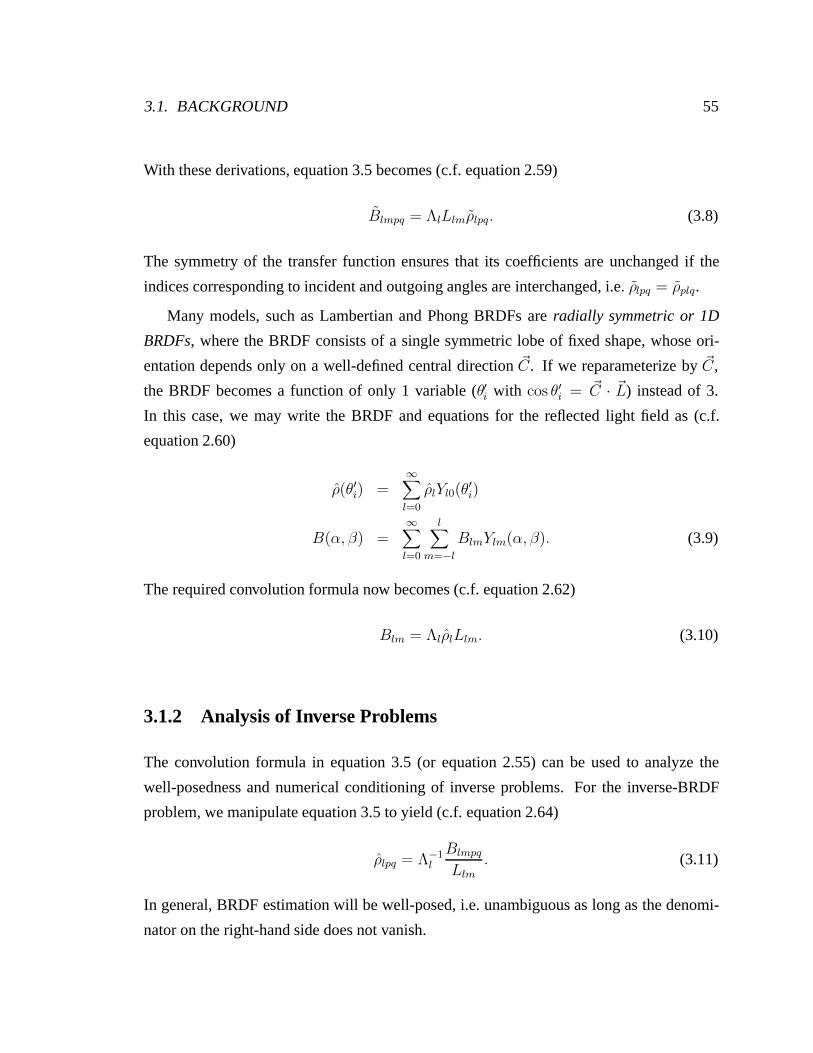
For a Lambertian surface, the BRDF is a constant, corresponding to the surface albedo—

which for purposes of energy conservation must not be greater than 1/π. For simplicity, we

will omit this constant in what follows. The transfer function is a clamped cosine since it

is equal to the cosine of the incident angle over the upper hemisphere when cos θ′i > 0 and

is equal to 0 over the lower hemisphere when cos θ′i < 0. A graph of this function, along

with spherical harmonic approximations to it up to order 4 is in figure 3.1.

0 0.5 1 1.5 2 2.5 3−0.4

−0.2

0

0.2

0.4

0.6

0.8

1Clamped Cosl=0 l=1 l=2 l=4

π/2 π

Figure 3.1: The clamped cosine filter corresponding to the Lambertian BRDF and successiveapproximations obtained by adding more spherical harmonic terms. For l = 2, we already get avery good approximation.

Since the reflected light field is proportional to the incident irradiance and is equal for

all outgoing directions, we will drop the outgoing angular dependence and use the form of

the convolution formula given in equation 3.10,

ρ = max(cos θ′i, 0) =∞∑l=0

ρlYl0(θ′i)



It remains to derive the form of the spherical harmonic coefficients ρl. To derive the spheri-

cal harmonic coefficients for the Lambertian BRDF, we must represent the transfer function

ρ(θ′i) = max(cos θ′i, 0) in terms of spherical harmonics.

We will need to use many formulas for representing integrals of spherical harmonics,

for which a reference [52] will be useful. The spherical harmonic coefficients are given by

ρl = 2π∫ π

2

0Yl0(θ

′i) cos θ

′i sin θ

′i dθ

′i. (3.29)

The factor of 2π comes from integrating 1 over the azimuthal dependence. It is important to

note that the limits of the integral range from 0 to π/2 and not π because we are considering

only the upper hemisphere. The expression above may be simplified by writing in terms of

Legendre polynomials P (cos θ′i). Putting u = cos θ′i in the above integral and noting that

P1(u) = u and that Yl0(θ′i) = Λ

−1l Pl(cos θ

′i), we obtain

ρl = 2πΛ−1l

∫ 1

0Pl(u)P1(u) du. (3.30)

To gain further insight, we need some facts regarding the Legendre polynomials. Pl is odd

if l is odd, and even if l is even. The Legendre polynomials are orthogonal over the domain

[−1, 1] with the orthogonality relationship being given by

∫ 1

−1Pa(u)Pb(u) =

2

2a+ 1δa,b. (3.31)

From this, we can establish some results about equation 3.30. When l is equal to 1, the

integral evaluates to half the norm above, i.e. 1/3. When l is odd but greater than 1, the

integral in equation 3.30 vanishes. This is because, for a = l and b = 1, we can break the

left-hand side of equation 3.31 using the oddness of a and b into two equal integrals from

[−1, 0] and [0, 1]. Therefore, both of these integrals must vanish, and the latter integral is

the right-hand integral in equation 3.30. When l is even, the required formula is given by

manipulating equation 20 in chapter 5 of MacRobert[52]. Putting it all together, we obtain,


l = 1 ρl =

√π

3l > 1, odd ρl = 0

l even ρl = 2π

√2l + 1

4π

(−1) l2−1

(l + 2)(l − 1)

[l!

2l( l2!)2

]. (3.32)

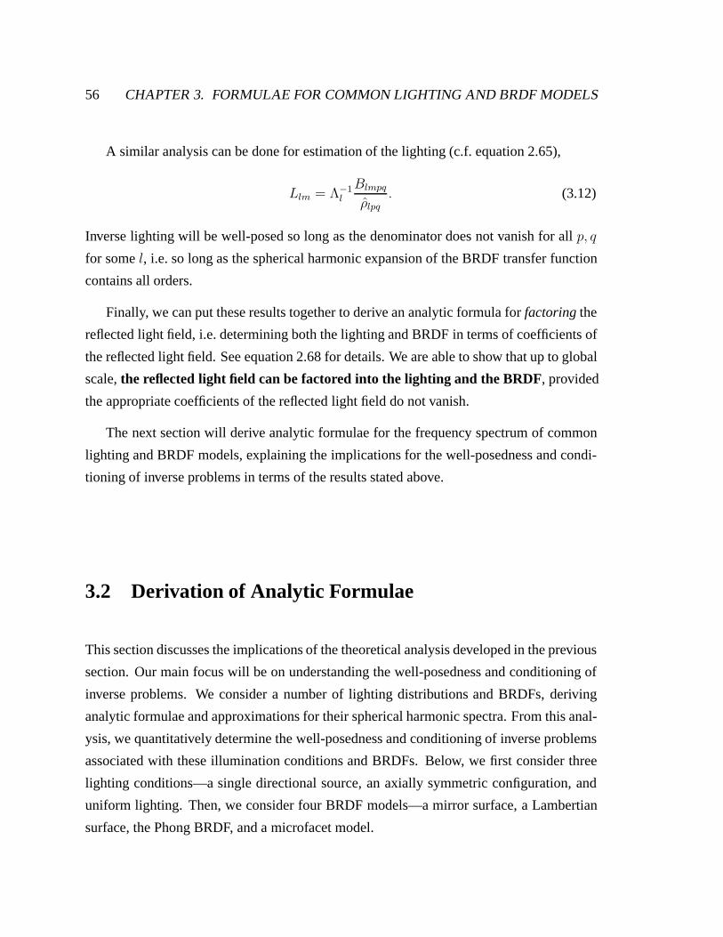
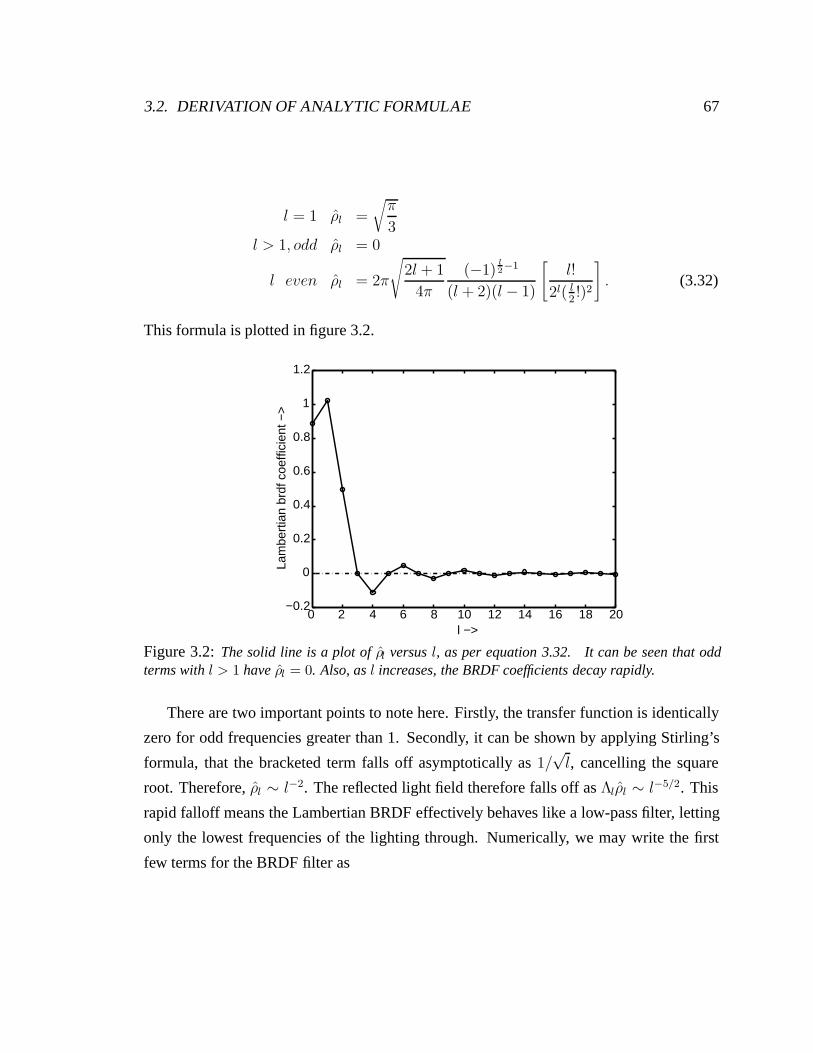
This formula is plotted in figure 3.2.

0 2 4 6 8 10 12 14 16 18 20−0.2

0

0.2

0.4

0.6

0.8

1

1.2

l −>

Lam

bert

ian

brdf

coe

ffici

ent −

>

Figure 3.2: The solid line is a plot of ρl versus l, as per equation 3.32. It can be seen that oddterms with l > 1 have ρl = 0. Also, as l increases, the BRDF coefficients decay rapidly.

There are two important points to note here. Firstly, the transfer function is identically

zero for odd frequencies greater than 1. Secondly, it can be shown by applying Stirling’s

formula, that the bracketed term falls off asymptotically as 1/√l, cancelling the square

root. Therefore, ρl ∼ l−2. The reflected light field therefore falls off as Λlρl ∼ l−5/2. This

rapid falloff means the Lambertian BRDF effectively behaves like a low-pass filter, letting

only the lowest frequencies of the lighting through. Numerically, we may write the first

few terms for the BRDF filter as


Λ0ρ0 = 3.142

Λ1ρ1 = 2.094

Λ2ρ2 = 0.785

Λ3ρ3 = 0

Λ4ρ4 = −0.131

Λ5ρ5 = 0

Λ6ρ6 = 0.049. (3.33)

We see that already for l = 4, the coefficient is only about 4% of what it is for l = 0. In

fact, it can be shown that over 99% of the energy of the BRDF filter is captured by l ≤ 2. By

considering the fact that the lighting must remain positive everywhere [2], similar worst-

case bounds can be shown for the approximation of the reflected light field by l ≤ 2.

Therefore, the irradiance, or equivalently, the reflected light field from a Lambertian

surface can be well approximated using only the first 9 terms of its spherical harmonic

expansion—1 term with order 0, 3 terms with order 1, and 5 terms with order 2. Note that

the single order 0 mode Y00 is a constant, the 3 order 1 modes are linear functions of the

Cartesian coordinates—in real form, they are simply x, y, and z—while the 5 order 2 modes

are quadratic functions of the Cartesian coordinates. Therefore, the irradiance can be well

approximated as a quadratic polynomial of the Cartesian coordinates of the surface normal

vector.

We first consider illumination estimation, or the inverse lighting problem. The fact that

the odd frequencies greater than 1 of the BRDF vanish means the inverse lighting prob-

lem is formally ill-posed for a Lambertian surface. The filter zeros the odd frequencies of

the input signal, so these terms cannot be estimated from images of a convex Lambertian

object. This observation corrects a commonly held notion (see Preisendorfer [67], volume

2, pages 143–151) that radiance and irradiance are equivalent in the sense that irradiance

can be formally inverted to recover the radiance. Different radiance distributions can give

rise to the same irradiance distribution. For further details, see [72]. Moreover, in practical


applications, we can robustly estimate only the first 9 coefficients of the incident illumina-

tion, those with l ≤ 2. Thus, inverse lighting from a Lambertian surface is not just formally

ill-posed for odd frequencies, but very ill-conditioned for even frequencies. This result ex-

plains the ill-conditioning observed by Marschner and Greenberg [54] in estimating the

lighting from a surface assumed to be Lambertian.

The 9 parameter approximation also gives rise to a simple algorithm (described in detail

in chapter 6) for estimating the illumination at high angular resolution from surfaces having

both diffuse and specular components. The diffuse component of the reflected light field

is subtracted out using the 9 parameter approximation for Lambertian surfaces. The object

is then treated as a gazing sphere, with the illumination recovered from the specular com-

ponent alone. A consistency condition ensures that the high frequency lighting recovered

from the specular BRDF component is indeed consistent with the low frequency lighting

used to subtract out the diffuse component of the reflected light field.

Our results are also in accordance with the perception literature, such as Land’s retinex

theory [46]. It is common in visual perception to associate lighting effects with low fre-

quency variation, and texture with high frequency variation. Our results formalize this

observation, showing that distant lighting effects can produce only low frequency varia-

tion, with respect to orientation, in the intensity of a homogeneous convex Lambertian

surface. Therefore, it should be possible to estimate high frequency texture independently

of the lighting. However, for accurate computational estimates as required for instance in

computer graphics, there is still an ambiguity between low frequency texture and lighting-

related effects.

Since the approximation of Lambertian surfaces is commonly used in graphics and

vision, the above results are of interest for many other problems. For instance, we can

simply use the first 9 terms of the lighting to compute the irradiance, i.e. the shading on

a Lambertian surface. Further implementation details on computing and rendering with

irradiance environment maps are found in chapter 4. The 9 parameter approximation also

means that images of a diffuse object under all possible illumination conditions lie close to

a 9D subspace. This is a step toward explaining many previous empirical observations of

the low-dimensional effects of lighting made in the computer vision community, such as

by Hallinan [30] and Epstein et al. [18]. Basri and Jacobs [2] have derived a Lambertian


formula similar to ours, and have applied this result to lighting invariant recognition, and

more recently to photometric stereo under general unknown lighting [3].

3.2.6 Phong BRDF

The normalized Phong transfer function is

ρ =s+ 1

2π

(R · L

)s, (3.34)

where R is the reflection vector, L is the direction to the light source, and s is the shininess,

or Phong exponent. The normalization ensures that the Phong lobe has unit energy. Tech-

nically, we must also zero the BRDF when the light vector is not in the upper hemisphere.

However, the Phong BRDF is not physically based anyway, so others have often ignored

this boundary effect, and we will do the same. This allows us to reparameterize by the

reflection vector R, making the transformations outlined in section 2.3.4 or at the end of

section 3.1.1. In particular, R · L → cos θ′i. Since the BRDF transfer function depends only

on R · L = cos θ′i, the Phong BRDF after reparameterization is mathematically analogous

to the Lambertian BRDF just discussed (they are both radially symmetric). In particular,

equation 3.28 holds. However, note that while the Phong BRDF is mathematically analo-

gous to the Lambertian case, it is not physically similar since we have reparameterized by

the reflection vector. The BRDF coefficients depend on s, and are given by

ρl = (s+ 1)∫ π/2

0[cos θ′i]

sYl0(θ

′i) sin θ

′i dθ

′i


To solve this integral, we substitute u = cos θ′i in equation 3.35. We also note that Yl0(θ′i) =

Λ−1l Pl(cos θ

′i), where Pl is the legendre polynomial of order l. Then, equation 3.35 becomes

ρl = Λ−1l (s+ 1)

∫ 1

0usPl(u) du. (3.36)


An analytic formula is given by MacRobert [52] in equations 19 and 20 of chapter 5,

ODD l Λlρl =(s+ 1)(s− 1)(s− 3) . . . (s− l + 2)

(s+ l + 1)(s+ l − 1) . . . (s+ 2)

EVEN l Λlρl =s(s− 2) . . . (s− l + 2)

(s+ l + 1)(s+ l − 1) . . . (s+ 3) . (3.37)

This can be expressed using Euler’s Gamma function, which for positive integers is simply

the factorial function, Γ(n) = (n − 1)!. Neglecting constant terms, we obtain for large s

and s > l − 1,

Λlρl =

[Γ(

s2

)]2Γ(

s2− l

2

)Γ(

s2+ l

2

) . (3.38)

If l s, we can expand the logarithm of this function in a Taylor series about l = 0.

Using Stirling’s formula, we obtain

log(Λlρl) = −l2(1

2s− 1

2s2

)+O

(l4

s2

). (3.39)

For large s, 1/s 1/s2, and we may derive the approximation

Λlρl ≈ exp

[− l2

2s

]. (3.40)

The coefficients fall off as a gaussian with width of order√s. The Phong BRDF behaves in

the frequency domain like a gaussian filter, with the filter width controlled by the shininess.

Therefore, inverse lighting calculations will be well-conditioned only up to order√s. As s

approaches infinity, Λlρl = 1, and the frequency spectrum becomes constant, correspond-

ing to a perfect mirror. Note that the frequency domain width of the filter varies inversely

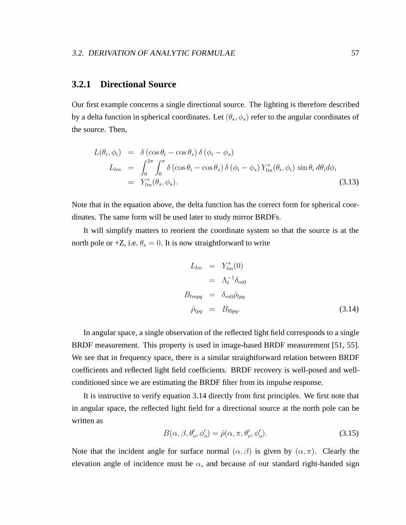
with the angular domain extent of the BRDF filter. A plot of the BRDF coefficients and the

approximation in equation 3.40 is shown in figure 3.3.

We should also note that for l > s, ρl vanishes if l and s are both odd or both even. It

can be shown that for l s, the nonzero coefficients fall off very rapidly as ρl ∼ l−(s+1).

This agrees with the result for the mathematically analogous Lambertian case, where s = 1

and ρl ∼ l−2. Note that s √s, so ρl is already nearly 0 when l ≈ s.


0 2 4 6 8 10 12 14 16 18 20−0.2

0

0.2

0.4

0.6

0.8

1

1.2

l −>

BR

DF

coe

ffici

ent −

>s=8 s=32 s=128 s=512

Figure 3.3: Numerical plots of the Phong coefficients Λlρl, as defined by equation 3.37. The solidlines are the gaussian filter approximations in equation 3.40. As the Phong exponent s increases,corresponding to increasing the angular width of the BRDF filter, the frequency width of the BRDFfilter decreases.

Associativity of Convolution: With respect to factorization of light fields with surfaces

approximated by Phong BRDFs, we obtain the same results for reflective surfaces as we did

for mirror BRDFs. From the form of equation 3.35, it is clear that there is an unrecoverable

scale factor for each order l. In physical terms, using the real BRDF and real lighting

is equivalent to using a blurred version of the illumination and a mirror BRDF. In signal

processing terminology, associativity of convolution allows us to sharpen the BRDF while

blurring the illumination without affecting the reflected light field. To be more precise, we

may rewrite equation 3.35 as

L′lm = ΛlρlLlm

Λlρ′l = 1

Blm = Λlρ′lL

′lm

= L′lm. (3.41)


These equations say that we may blur the illumination using the BRDF filter, while treat-

ing the BRDF as a mirror. This formulation also allows us to analyze the conditioning in

estimating the parameters of a Phong BRDF model under arbitrary illumination. The form

of equation 3.40 for the Phong BRDF coefficients indicates that for l √s, the effects of

the filtering in equation 3.41 are minimal. The BRDF filter passes through virtually all the

low-frequency energy with practically no attenuation. Thus, under low-frequency lighting,

the reflected light field is essentially independent of the Phong exponent s. This means

that under low-frequency lighting, estimation of the exponent s of a Phong BRDF

model is ill-conditioned. In physical terms, it is difficult to determine the shininess of

an object under diffuse lighting. In order to do so robustly, we must have high-frequency

lighting components like directional sources. This observation holds for many reflective

BRDF models. In particular, we shall see that a similar result can be derived for micro-

facet BRDFs; estimation of the surface roughness is ill-conditioned under low-frequency

lighting.

3.2.7 Microfacet BRDF

Consider a simplified Torrance-Sparrow [84] model,

ρ =1

4πσ2 cos θ′i cos θ′o

exp

−

(θ′hσ

)2 . (3.42)

The subscript h stands for the half-way vector, while σ corresponds to the surface roughness

parameter. For simplicity, we have omitted Fresnel and geometric shadowing terms, as well

as the Lambertian component usually included in such models.

It is convenient to reparameterize by the reflection vector, as we did for the Phong

BRDF. However, it is important to note that microfacet BRDFs are not symmetric about

the reflection vector. Unlike for the Phong BRDF, there is a preferred direction, determined

by the exitant angle. However, it can be shown by Taylor-series expansions and verified

numerically that it is often reasonable to treat the microfacet BRDF using the same ma-

chinery as for the Phong case, assuming no outgoing angular dependence. Even under this

assumption, it is somewhat difficult to derive precise analytic formulae. However, we may


make good approximations.

We analyze the microfacet BRDF by fixing the outgoing angle and reparameterizing

by the reflection vector. That is, we set the outgoing angle to (θ′o, 0), corresponding to an

angle of 2θ′o with respect to the reflection vector. We now write the BRDF as

ρ =∞∑l=0

l∑q=−l

ρlq(θ′o)Ylq(θ

′i, φ

′i). (3.43)

Note that we have reparameterized with respect to the reflection vector, so θ′i refers to the

angle made with the reflection vector. Our goal is to show that azimuthally dependent

terms, i.e. those with q = 0 are small, at least for small angles θ′o. Furthermore, we would

like to find the forms of the terms with q = 0. We start off by considering the simplest

case, i.e. θ′o = 0. This corresponds to normal exitance, with the reflection vector also

being normal to the surface. We then show how Taylor series expansions can be used to

generalize the results.

Normal Exitance

For normal exitance, there is no azimuthal dependence, and the half angle, θ′h = θ′i/2,

ρl = 2π∫ π/2

0

exp[−θ′i

2/4σ2]

4πσ2Yl0(θ

′i) sin θ

′i dθ

′i. (3.44)

The expansion of Yl0(t) near t = 0 for small l is

Yl0(t) = Λ−1l

(1− l(l + 1)

4t2 +O(t4)

). (3.45)

The asymptotic form of Yl0(t) near t = 0 for large l is

Yl0(t) ∼ Λ−1l

(1√tcos[(l + 1/2)t− π/4]

). (3.46)

To integrate equation 3.44, we substitute u = θ′i/2σ. Then, θ′i = 2σu. Assuming σ 1,

as it is for most surfaces, the upper limit of the integral becomes infinite, and we have that


sin θ′i dθ′i = θ′i dθ

′i = 4σ

2u du,

ρl =∫ ∞

02e−u2

Yl0(2σu)u du. (3.47)

We therefore set t = 2σu in equations 3.45 and 3.46. When σl 1, we use equation 3.45

to obtain to O([σl]4),

Λlρl =(∫ ∞

02ue−u2

d u− (σl)2∫ ∞

02u3e−u2

du). (3.48)

Substituting, v = u2, both integrals evaluate to 1, so we obtain

Λlρl = 1− (σl)2 +O([σl]4

). (3.49)

We note that these are the first terms of the Taylor series expansion of exp[−(σl)2]. When

σl 1, we use equation 3.46 to obtain (Φ is a phase that encapsulates the lower-order

terms)

Λlρl ∼∫ ∞

0e−u2√

u cos[(2σl)u+Φ] du. (3.50)

The dominant term can be shown to be exp[−(2σl)2/4] = exp[−(σl)2]. Therefore, we

can simply use exp[−(σl)2] as a valid approximation in both domains, giving rise to an

approximation of the form

Λlρl ≈ exp[− (σl)2

]. (3.51)

We have also verified this result numerically.

For normal exitance, the BRDF is symmetric about the reflection vector and gaussian,

so in that case, equation 3.51 simply states that even in the spherical-harmonic basis, the

frequency spectrum of a gaussian is also approximately gaussian, with the frequency width

related to the reciprocal of the angular width. For non-normal exitance, we will see that

this is still a good approximation. The corrections are small except when l is large (corre-

sponding to directional light sources), and at large viewing angles. These statements are

made more precise in the next subsection.


Non-Normal Exitance

For non-normal exitance, we first expand θ′h in a Taylor series in terms of θ′i. After some

tedious manipulation, we can verify that to first order,

θ′h2=

(θ′i2

)2 (1 + sin2 φ′

i tan2 θ′o

). (3.52)

When θ′o = 0 (normal exitance), this is the result we obtained earlier. When θ′o = 0, there is

some asymmetry, and the half-angle depends on the azimuthal angle between the light and

viewing vector, as defined by the formula above. In angular-space, the BRDF behaves as

an “anisotropic” filter over the incident illumination. Our goal here is to bound the extent

of this “anisotropy”, or asymmetry.

We first consider the coefficients for the isotropic or azimuthally symmetric term Yl0.

For l small, we can expand as 1− (σl)2+O(σl)4. Now, the constant term is just the area of

the microfacet distribution, but when normalized by cos θ′o must integrate to 1. Therefore,

corrections are at least of O(θ′o2(σl)2). In fact, it is possible to obtain a tighter bound by

deeper analysis.

Therefore, these corrections are not significant for small outgoing angles, and within

that domain, we may use equation 3.51 as a good approximation. It should be noted that

in practical applications, measurements made at wide or near-grazing angles are given low

confidence anyway.

To make this more concrete, consider what happens to equation 3.47. Considering the

first term in the Taylor-series expansion, and including the cos θ′o term in the denominator,

we get

ρl =1

cos θ′o

∫ ∞

02ue−u2

Yl0(2σu)

(1− u2 tan2 θ′o

2

)du. (3.53)

The factor of 2 in the denominator of the last (correction) term is to take care of the inte-

gration of sin2 φ′i. Next, we expand both the cosine and tangent functions about θ′o = 0,

i.e. cos θ′o = 1− θ′o2/2 + O

(θ′o

4)

and tan2 θ′o = θ′o2 + O

(θ′o

4). Upon doing this, it can be

verified that, as expected from physical arguments, there is no net correction to the integral

and equation 3.53 evaluates to equation 3.49.


Now, consider the anisotropic terms Ylq with q = 0. If we Taylor expand as in equa-

tion 3.53, we are again going to get something at least of O(θ′o

2), and because the Ylq

constant term vanishes, there will be another factor of σ. In fact, if we Taylor-expand, we

get an expansion of the form sin2 φ′i+sin

4 φ′i+ · · · and it is clear that the azimuthal integral

against Ylq vanishes unless there is a term of type sinq φ′i. Therefore, the corrections are ac-

tually O (θ′oqσ). What this means in practice is that the azimuthally dependent corrections

are only important for large viewing angles and large orders l (l must be large if q is large,

and for small q, θ′oqσ is small for σ 1 even if θ′o is large).

But, that situation will arise only for observations made at large angles of lights that

have broad spectra, i.e. directional sources. Therefore, these should be treated separately,

by separating the illumination into slow and fast varying components. Equation 3.51 in

the frequency domain is a very good approximation for the slow-varying lighting compo-

nent, while we may approximate the fast-varying lighting component using one or more

directional sources in the angular domain.

Conditioning Properties

Since equation 3.51 has many similarities to the equations for the Phong BRDF, most of

those results apply here too. In particular, under low-frequency lighting, there is an am-

biguity with respect to estimation of the surface roughness σ. Also, inverse lighting is

well-conditioned only up to order σ−1. With respect to factorization, there are ambigui-

ties between illumination and reflectance, similar to those for mirror and Phong BRDFs.

Specifically, we may blur the illumination while sharpening the BRDF. However, it is im-

portant to note that while these ambiguities are exact for Phong and mirror BRDFs, they

are only a good approximation for microfacet BRDFs since equation 3.51 does not hold at

grazing angles or for high-frequency lighting distributions. In these cases, the ambiguity

can be broken, and we have used this fact in an algorithm to simultaneously determine the

lighting and the parameters of a microfacet model [73].

In summary, while it is difficult to derive precise analytic formulae, we can derive good

approximations to the frequency-space behavior of a microfacet BRDF model. The results

are rather similar to those for the Phong BRDF with the Phong exponent s replaced by the


physically-based surface roughness parameter σ.

In this subsection, we have seen analytic formulae derived for a variety of common

lighting and BRDF models, demonstrating the implications of the theoretical analysis. We

end this chapter by summarizing its key contributions, discussing avenues for future work,

and outlining the rest of the dissertation, which discusses some practical applications of the

theoretical analysis in chapters 2 and 3.

3.3 Conclusions and Future Work

We have presented a theoretical analysis of the structure of the reflected light field from a

convex homogeneous object under a distant illumination field. In chapter 2, we have shown

that the reflected light field can be formally described as a convolution of the incident

illumination and the BRDF, and derived an analytic frequency space convolution formula.

This means that, under our assumptions, reflection can be viewed in signal processing terms

as a filtering operation between the lighting and the BRDF to produce the output light field.

Furthermore, inverse rendering to estimate the lighting or BRDF from the reflected light

field can be understood as deconvolution. This result provides a novel viewpoint for many

forward and inverse rendering problems.

In this chapter, we have derived analytic formulae for the frequency spectra of many

common BRDF and lighting models, and have demonstrated the implications for inverse

problems such as lighting recovery, BRDF recovery, and light field factorization. We have

shown in frequency-space why a gazing sphere is well-suited for recovering the lighting—

the frequency spectrum of the mirror BRDF (a delta function) is constant—and why a

directional source is well-suited for recovering the BRDF—we are estimating the BRDF

filter by considering its impulse response. With the aid of our theory, we have been able

to quantitatively determine the well-posedness and conditioning of many inverse problems.

The ill-conditioning observed by Marschner and Greenberg [54] in estimating the lighting

from a Lambertian surface has been explained by showing that only the first 9 coefficients

of the lighting can robustly be recovered, and we have shown that factorization of lighting

effects and low-frequency texture is ambiguous. All these results indicate that the theory

3.3. CONCLUSIONS AND FUTURE WORK 79

provides a useful analytical tool for studying the properties of inverse problems.

Of course, all the results presented in this chapter depend on our assumptions. Further-

more, the results for well-posedness of inverse problems depend on having all the reflected

light field coefficients, or the entire reflected light field available. It is an interesting future

direction to consider how these results change when we have only a limited fraction of the

reflected light field available, as in most practical applications, or can move our viewpoint

only in a narrow range. More generally, we believe a formal analysis of inverse problems

under more general assumptions is of significant and growing interest in many areas of

computer graphics, computer vision, and visual perception.

The remainder of this dissertation describes practical applications of the theoretical

framework for forward and inverse rendering. Chapters 4 and 5 describe frequency domain

algorithms for environment map prefiltering and rendering. Chapter 4 discusses the case

of Lambertian BRDFs (irradiance maps), while chapter 5 extends these ideas to the gen-

eral case with arbitrary isotropic BRDFs. Finally, chapter 6 discusses how the theoretical

analysis can be extended and applied to solve practical inverse rendering problems under

complex illumination.

Documents

Chapter 3 Formulae for Common Lighting and BRDF … 3 Formulae for Common Lighting and BRDF Models An analysis of the computational properties of the reﬂection operator is of interest