128

Chapter 3

Clustering Wireless Sensor Nodes Using Caterpillar Graph

3. Introduction

A wireless sensor network is a collection of nodes organized into a cooperative

network [1].Currently, wireless sensor networks are beginning to be deployed at an

accelerated space. It is not unreasonable to expect that in 10-15 years that the world

will be covered with wireless sensor networks with access to them via the Internet.

This can be considered as the Internet becoming a physical network. This new

technology is exciting with unlimited potential for numerous application areas

including environmental, medical, military, transportation, entertainment, crisis

management, homeland defense, and smart spaces. Since a wireless sensor network is

a distributed real-time system a natural question is how many solutions from

distributed and real-time systems can be used in these new systems? Unfortunately,

very little prior work can be applied and new solutions are necessary in all areas of

the system. The main reason is that the set of assumptions underlying previous work

has changed dramatically. Most past distributed systems research has assumed that the

systems are wired, have unlimited power, are not real-time, have user interfaces such

as screens and mice, have a fixed set of resources, treat each node in the system as

very important and are location independent. In contrast, for wireless sensor networks,

the systems are wireless, have scarce power, are real-time, utilize sensors and

actuators as interfaces, have dynamically changing sets of resources, aggregate

behavior is important and location is critical. Many wireless sensor networks also

129

utilize minimal capacity devices which places a further strain on the ability to use past

solutions.

3.1 MAC

A medium access control (MAC) protocol coordinates actions over a shared channel.

The most commonly used solutions are contention-based. One general contention-

based strategy is for a node which has a message to transmit to test the channel to see

if it is busy, if not busy then it transmits, else if busy it waits and tries again later.

After colliding, nodes wait random amounts of time trying to avoid re-colliding. If

two or more nodes transmit at the same time there is a collision and all the nodes

colliding try again later. Many wireless MAC protocols also have a dozen mode

where nodes not involved with sending or receiving a packet in a given timeframe go

into sleep mode to save energy. Many variations exist on this basic scheme. In

general, most MAC protocols optimize for the general case and for arbitrary

communication patterns and workloads. However, a wireless sensor network has more

focused requirements that include a local unicast or broad cast , traffic is generally

from nodes to one or a few sinks (most traffic is then in one direction),have periodic

or rare communication and must consider energy consumption as a major factor. An

effective MAC protocol for wireless sensor networks must consume little power,

avoid collisions, be implemented with a small code size and memory requirements, be

efficient for a single application, and be tolerant to changing radio frequency and

networking conditions. One example of a good MAC protocol for wireless sensor

networks is B-MAC [2]. B-MAC is highly configurable and can be implemented with

130

a small code and memory size. It has an interface that allows choosing various

functionality and only that functionality as needed by a particular application. B-MAC

consists of four main parts: clear channel assessment (CCA), packet back off, link

layer acks, and low power listening. For CCA, B-MAC uses a weighted moving

average of samples when the channel is idle in order to assess the background noise

and better be able to detect valid packets and collisions. The packet back off time is

configurable and is chosen from a linear range as opposed to an exponential back off

scheme typically used in other distributed systems. This reduces delay and works

because of the typical communication patterns found in a wireless sensor network. B-

MAC also supports a packet by packet link layer acknowledgement. In this way only

important packets need pay the extra cost. A low power listening scheme is employed

where a node cycles between awake and sleep cycles. While awake it listens for a

long enough preambles to assess if it needs to stay awake or can return to sleep mode.

This scheme saves significant amounts of energy. Many MAC protocols use a request

to send (RTS) and clear to send (CTS) style of interaction. This works well for ad hoc

mesh networks where packet sizes are large (1000s of bytes). However, the overhead

of RTS-CTS packets to set up a packet transmission is not acceptable in wireless

sensor networks where packet sizes are on the order of 50 bytes. B-MAC, therefore,

does not use a RTS-CTS scheme. Recently, there has been new work on supporting

multi-channel wireless sensor networks. In these systems it is necessary to extend

MAC protocols to multi-channel MACs. One such protocol is MMSN[3] . These

protocols must support all the features found in protocols such as B-MAC, but must

also assign frequencies for each transmission. Consequently, multi-frequency MAC

131

protocols consist of two phases: channel assignment and access control. The details

for MMSN are quite complicated and are not described here. On the other hand, we

expect that more and more future wireless sensor networks will employ multiple

channels (frequencies). The advantages of multi-channel MAC protocols include

providing greater packet throughput and being able to transmit even in the presence of

a crowded spectrum.

3.1.1 Routing

Semantics may be that a single node closest to the geographic destination is to be the

unicast node. Second, the semantics could be that all nodes within some area around

the destination address should receive the message. This is an area multicast. Third, it

may only be necessary for any node, called any cast, in the destination area to receive

the message. The SPEED [4] protocol supports these 3 types of semantics. There is

also often a need to flood (multicast) to the entire network. Many routing schemes

exist for supporting efficient flooding.

Real-Time: For some applications, messages must arrive at a destination by a

deadline. Due to the high degree of uncertainty in WSN it is difficult to develop

routing algorithms with any guarantees. Protocols such as SPEED [5] and RAP [6]

use a notion of velocity to prioritize packet transmissions. Velocity is a nice metric

that combines the deadline and distance that a message must travel.

Mobility: Routing is complicated if either the message source or destination or both

are moving. Solutions include continuously updating local neighbor tables or

identifying proxy nodes which are responsible for keeping track of where nodes are.

132

Proxy nodes for a given node may also change as a node moves further and further

away from its original location.

Voids: Since WSN nodes have a limited transmission range, it is possible that for

some node in the routing path there are no forwarding nodes in the direction a

message is supposed to travel. Protocols like GPSR [7]. Solve this problem by

choosing some other node “not” in the correct direction in an effort to find a path

around the void.

Security: If adversaries exist, they can perpetrate a wide variety of attacks on the

routing algorithm including selective forwarding, black hole, Sybil, replays,

wormhole and denial of service attacks. Unfortunately, almost all WSN routing

algorithms have ignored security and are vulnerable to these attacks. Protocols such as

SPINS [8] have begun to address secure routing issues.

Congestion: Today, many WSN have periodic or infrequent traffic. Congestion does

not seem to be a big problem for such networks. However, congestion is a problem

for more demanding WSN and is expected to be a more prominent issue with larger

systems that might process audio, video and have multiple base stations (creating

more cross traffic). Even in systems with a single base station, congestion near the

base station is a serious problem since traffic converges at the base station. Solutions

use backpressure, reducing

133

3.2 Design Challenges

Several design challenges present themselves to designers of wireless sensor network

applications. The limited resources available to individual sensor nodes implies

designers must develop highly distributed, fault-tolerant, and energy efficient

applications in a small memory-footprint. Some features of wireless sensor nodes are:

1. Individual nodes in a wireless sensor network have limited computational power

and storage capacity. They operate on nonrenewable power sources and employ a

short-range transceiver to send and receive messages.

2. The number of nodes in a wireless sensor network can be several orders of

magnitude higher than in an ad hoc network. Thus, algorithm scalability is an

important design criterion for sensor network applications.

3. Sensor nodes are generally densely deployed in the area of interest. This dense

deployment can be leveraged by the application, since nodes in close proximity can

collaborate locally prior to relaying information back to the base station.

4. Sensor networks are prone to frequent topology changes. This is due to several

reasons, such as hardware failure, depleted batteries, intermittent radio interference,

environmental factors, or the addition of sensor nodes. As a result, applications

require a degree of inherent fault tolerance and the ability to reconfigure themselves

as the network topology evolves over time.

Wireless sensor networks do not employ a point-to-point communication paradigm

because they are usually not aware of the entire size of the network and nodes are not

uniquely identifiable. Consequently, it is not possible to individually address a

specific node. Paradigms, such as directed diffusion [9, 10] employ a data-centric

134

view of generated sensor data. Nodes request data by disseminating interests for this

named data throughout the network. Data that matches the criterion are relayed back

toward the querying node.

Even with the limitations individual sensor nodes possess and the design challenges

application developers face, several advantages exist for instrumenting an area with a

wireless sensor network [11].Due to the dense deployment of a greater number of

nodes, a higher level of fault tolerance is achievable in wireless sensor networks. .

Coverage of a large area is possible through the union of coverage of several small

sensors. Coverage of a particular area and terrain can be shaped as needed to

overcome any potential barriers or holes in the area under observation. It is possible to

incrementally extend coverage of the observed area and density by deploying

additional sensor nodes within the region of interest. An improvement in sensing

quality is achieved by combining multiple, independent sensor readings. Local

collaboration between nearby sensor nodes achieves a higher level of confidence in

observed phenomena. . Since nodes are deployed in close proximity to the sensed

event, this overcomes any ambient environmental factors that might otherwise

interfere with observation of the desired phenomenon.

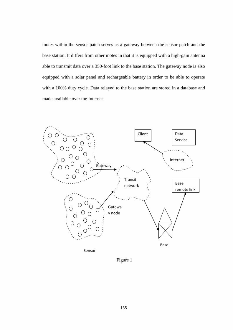
3.2.1 Architecture

The wireless sensor network architecture is divided into distinct tiers Fig. 1. The

lowest level consists of autonomous motes, equipped with various sensors that

perform basic networking, computing, and sensing tasks. They are organized into a

local one-hop network and collectively identified as a sensor patch. One of the sensor

135

motes within the sensor patch serves as a gateway between the sensor patch and the

base station. It differs from other motes in that it is equipped with a high-gain antenna

able to transmit data over a 350-foot link to the base station. The gateway node is also

equipped with a solar panel and rechargeable battery in order to be able to operate

with a 100% duty cycle. Data relayed to the base station are stored in a database and

made available over the Internet.

Client Data Service

Base remote link

Transit network

Base Sensor

Gateway node

Internet Gateway

Figure 1

136

3.3 Clustering

Clustering analysis is desirable in nearly any field of study where it is beneficial to

group data into similar sets depending on one’s objective in analyzing a set of data

one might define similarity between elements differently and thus a clustering process

could be optimized to provide numerous way of grouping a set of elements. In order

to create any sort of clustering algorithm and determine its effectiveness it is

necessary to find some way to quantity similarity between elements. When sensor

nodes are organized in clusters they could use either single hop or multi hop mode of

communication to send their data to their respective cluster heads. The sensor nodes

are randomly and uniformly distributed over the region and the nodes are organized in

clusters to take advantage of possible data aggregation at the cluster head nodes.

There are two types of nodes; cluster head nodes and sensor nodes. The cluster head

nodes act as the fusion points within the network. During each data gathering cycle

the sensor nodes send their sensed data to the closest cluster head node which perform

data aggregation. Then the cluster head directly transmits the aggregated data to a

base station. The sensor nodes have simple functionality, since they perform sensing

and relatively short-range communication. However the cluster head nodes are more

complex, since they coordinate MAC and routing within their cluster perform data

fusion and perform long range transmissions to the remote base station. The overall

system design problem involves determining the optimum number of cluster head

nodes the optimum node of communication within a cluster (Single hop or Multi

hop).Some of the objectives of the clustering nodes are as follows

137

• Involves grouping nodes into clusters and electing a CH

• Members of a cluster can communicate with their CH directly

• CH can forward the aggregated data to the central base station through

other CHs

• Clustering Objectives

• Allows aggregation

• Limits data transmission

• Facilitate the reusability of the resources

• CHs and gateway nodes can form a virtual backbone for intercluster

routing

• Cluster structure gives the impression of a smaller and more stable

network

• Improve network lifetime

• Reduce network traffic and the contention for the channel

• Data aggregation and updates take place in CHs

Various clustering algorithms have been proposed to organize sensor nodes in a

wireless sensor network into clusters. [1][2][3][4][5][6](Papers). Each aim to meet

certain needs of the system. This could provide a system having low clustering related

maintenance cost or energy efficient clusters to minimize energy consumption

suitable for sensor nodes with energy constraints or for load balancing to distribute

the workload of a network. The fig2 illustrates the concept of clusters.

138

Wireless sensor networks are networks of wireless nodes that are deployed over an area for

the purpose of monitoring certain phenomena of interest. The nodes perform certain

measurements process the measured data and transmit the processed data to a base station

over a wireless channels. The base station collects data from all the nodes and analyzes this

data to draw conclusion about the activity in the area of interest. These networks are different

from the traditional wireless ad hoc networks. However, when nodes are organized in clusters

and when they use multi hop communication to reach the cluster head the nodes closer to a

cluster head have a higher load of relaying packets as compared to other nodes. However is

Cluster member

Clusterhead

Gateway node

Intra - Cluster Cross - Cluster

Figure 2

139

most sensor networks nodes are static consequently the nodes closer to the cluster head get

overburdened constantly. The cluster heads themselves have the extra burden of performing

long rang transmissions to the distant base station.

We consider a region to be covered by sensor nodes. The number of sensor nodes is

determined by the application requirements. Usually each sensor node has a sensing radius

and it is required that the sensor nodes provide coverage of the region with a high probability.

The sensing radius of each node depends on the phenomenon that is being sensed as well as

the sensing hardware of the node. Thus in general the required number of sensor nodes is

dictated by the application and hence we assume it to be a constant.

3.3.1 Clustering Algorithm

Consider a wireless network represented by a connected graph where the

vertex set contains nodes and is the edge set. We assume that the nodes form

clusters in such a manner that the following assumptions are satisfied: . Each node

belongs to one and only one cluster.2. In each cluster, there is a node which is

adjacent to all the remaining nodes in the cluster. Such a node is called a cluster-head.

(If more than one such nodes exist, only one is chosen). Two clusters are called

adjacent (or neighbors) if there is a direct link joining them. Assume that through

some information exchange, a cluster-head knows all its neighboring clusters. In the

case that two clusters are joined by more than one links, we assume that the cluster-

heads of both clusters agree on a single such link being activated. The end nodes of

active links are called gateway nodes. The set of cluster-heads by our assumption is a

dominating set, i.e., a subset of nodes which are at most 1 hop away from any node.

140

The well-known minimum dominating set (MDS) problem seeks a dominating set of

minimum size, and has been proven to be -hard. In the following, we describe

hence its degree (i.e., the number of neighbors). Initially, a non-iterative

decentralized clustering algorithm for choosing a dominating set. Assume that each

node knows its one-hop neighbors, each node sets its own flag to , meaning that it

does not yet belong to any cluster. At a certain time, each node starts a timer with

length drawn from an exponential distribution with rate If node ’s timer expires

at , it becomes a cluster-head. It sets its flag to , and broadcasts a “cluster

initialize” message to all its neighbors. Each of its neighbors with flag signals its

intention to join the cluster by replying with a “cluster join” message. It also sets its

own flag to and stops the timer. At the end, clusters satisfying the two properties

mentioned above are formed. The particular choice of timers ensures that high degree

nodes have more chances to become cluster-heads, somewhat like a greedy algorithm.

3.4 Graph Terminology

We use an undirected graph with edges and nodes, to represent a

snapshot of the wireless sensor network. Each node in represents a mobile host, and

each edge in signifies that two hosts are within transmission range of each other.

The topology of is the set of edges and nodes. Hence, when we say a node

movement changes the topology, we mean a change in the network that results in a

change in either or . Specifically, an edge deletion occurs when two hosts lose

communication with each other, and an edge insertion occurs when two hosts move

141

into range of each other. A node deletion in isolation occurs when a host turns off its

power, and a node insertion in isolation occurs when a host turns on its power. By “in

isolation” we mean that no other change has occurred in the network. Because a node

insertion or deletion affects multiple edges, we process these changes to as multiple

changes to . Finally, the most general node movement models the movement of a

host from one part of the network to another; hence, a node movement is a

combination of a node deletion from one part of and a node insertion in another part

of . The open neighborhood of node represents all hosts within

transmission range of except for itself. The closed neighborhood of also

includes , that is, . With these definitions extended to subsets of

, the open neighborhood of ∈ , and the closed

neighborhood of is . The degree of v is the size of its open

neighborhood: The maximum degree of is ∈ For

the purposes of analysis of overhead, we assume that a local broadcast takes

time (which is true if the MAC layer can schedule local broadcasts reliably). Given a

subgraph of , the –degree of is , the number of ’s neighbors that are in

. The maximum degree of is denoted . The diameter of is the

maximum number of edges contained in any simple path between two nodes in .

The diameter of a subgraph of is denoted

We use an approximation to a minimum connected dominating set (MCDS). A

subset is a dominating set if . Let be the subgraph induced by

is a connected dominating set if, in addition to , is

142

connected. Since finding an MCDS is an -complete problem that is also hard to

approximate we present a distributed greedy MCDS approximation algorithm that is

similar to the algorithm in. The MCDS nodes are incidentally also the interior nodes

of a maximum leaf spanning tree.

We use the interior of this tree as the back bone. Thus, each node in has a unique

dominator in , denoted .The set ∈ is a maximum leaf

spanning tree. The nodes of comprise the interior of this spanning tree, and the

edges of this spanning tree between nodes in are called back bone edges. Wireless

sensor networks can be deployed for many application unlike wired networks or

cellular networks no physically backbone infrastructure is installed in wireless sensor

networks. A communication session is achieved either through a single hop if the

communication parties are close enough or through relating by intermediate nodes

otherwise. The topology of such wireless ad hoc network can be modeled as a unit

disk graph a geometric graph in which there is an edge between two nodes if and only

if there distance is at one unit as show in fig 3

Figure 3

143

Although a wireless sensor network has no physical backbone infrastructure a virtual

back bone can be formed by nodes in a connected dominating set of the corresponding

unit disk graph [6][7][8]. Such a virtual backbone plays a very important role in

routing, broadcasting, and connectivity managements in wireless sensor networks

3.4.1 Clustering Using Dominating Sets

A dominating set is a subset of a graph such that every vertex in is either in

or adjacent to a vertex in [12]. Dominating sets are widely used in clustering

networks [8]. Dominating sets can be classified into three main classes, Independent

Dominating Sets (IDS), Weakly Connected Dominating Sets (WCDS) and Connected

Dominating Sets (CDS) [13]

Independent Dominating Sets: IDS is a dominating set of a graph in which there

are no adjacent vertices.

Weakly Connected Dominating Sets (WCDS): A weakly induced sub graph is a

subset of a graph that contains the vertices of , their neighbors and all edges of

the original graph with at least one endpoint in . A subset is a weakly-connected

dominating set, if is dominating and is connected [14].

Connected Dominating Sets: A connected dominating set (CDS) is a subset of a

graph such that forms a dominating set and is connected.

Clustering Using IDS: Baker and Ephremides [15] proposed an independent

dominating set algorithm called highest vertex ID. A very similar algorithm to the

highest id algorithm is the lowest id algorithm by Gerla and Tsai [16].”Gerla and

Tsai” developed another algorithm to find the independent dominating sets called the

144

highest degree algorithm. Although these algorithms are considered as important

algorithms, Chen et al. [17] proposed that these algorithms are not working correctly

for some graphs. To solve this incorrect operation, Chen et al developed the -

distance independent dominating set algorithm.[18].

Clustering Using WCDS: Although independent dominating sets are suitable for

constructing optimum sized dominating sets, they have some deficiencies such as lack

of direct communication between cluster heads. In order to obtain the connectivity

between cluster heads, WCDSs can be used to construct clusters. A Dominating Set

Based Clustering Algorithm for Mobile Ad Hoc Networks 573. The WCDS was first

proposed for clustering in ad hoc networks by Chen and Liestman [19] called zonal

clustering.

Clustering Using CDS: CDS have many advantages in network applications such as

ease of broadcasting and constructing virtual backbones [20],however, when we try to

obtain a connected dominating set, we may have undesirable number of cluster heads.

So, in constructing connected dominating sets, our primary problem is to find a

minimal connected dominating set. Guha and Khuller [21] proposed two centralized

greedy algorithms for finding suboptimal connected dominating sets. Das and

Bharghavan [22] provided distributed implementations of Ghua and Khuller’s

algorithms [23]. Wu and Li [24] improved Das and Bhraghavan’s distributed

algorithm as a localized distributed algorithm for finding connected and Ophir

Frieder [25] proposed a distributed algorithm for finding a CDS which constructs the

dominating set using the Maximal Independent Sets. Hui Liu, Yi Pan and Jiannong

Cao [26],”Improved Wu and Li’s algorithm” [27] by adding a third phase elimination.

145

In the additional third phase, the algorithm searches redundant cluster heads. A cluster

head is eliminated if it is dominated by two of its cluster head neighbors.

3.5 Caterpillar Graphs

A caterpillar graph is a tree having a chordless path , called the backbone

that contains at least one end point of every edge. Edges connecting the leaves with

the backbone are called hairs. In a complete caterpillar graph, each vertex of its

backbone has a nonempty set of hairs denoted by a complete caterpillar graph

with backbone .

We can use a simple graph to represent an wireless sensor network,

where represents a set of wireless mobile hosts and represents a set of edges. An

edge between host pairs indicates that both hosts and are within their

wireless transmitter ranges. To simplify our discussions, we assume all mobile hosts

are homogeneous i.e. their wireless transmitter ranges are the same. In other word, if

there is an edge in E, it indicates is within ’s range and is within ’s

range. Thus the corresponding graph will be an undirected graph. The graph in fig3

represents the corresponding wireless sensor network.

Figure 4

146

Lemma 1 ([28]). If is a chord less path with vertices, then

≥ two vertices

are twins in a graph if they have the same neighborhood. Jou et al [28] proved the

following properties.

Lemma 2. If and are twins in a graph then

Lemma 3. If is an induced subgraph of , then

Lemma 4. ([29]) For any two disjoint graphs and Let

For each , ) is the set of its

pendent vertices and is an independent set but it

is not maximal in If same vertex of belongs to a MIS then every vertex

of ) must belongs to it otherwise it is not maximal. As two vertices of are

twins in , we can construct them in to a single vertex, called hi, that represents

the whole set . Let be the construction group of

otherwise that is also a caterpillar graph with at most one pendent vertex at

each the contraction graph of a complete caterpillar graph is also complete.

Here, we can deploy the wireless sensor nodes in the form of caterpillar graphs as

shown in the fig. 4.But our objective here is to retain the connected dominating set

from the caterpillar graphs. Because the nodes in the set of connected dominating set

are cluster heads which has many applications in wireless sensor networks.We are

using linear algorithm to retain connected dominating set (CDS).

147

3.6 Linear Algorithm

Efficient liner algorithm for the domination number of a tree designed by

Cockayne,S Goodman and S Hedetniemi Cock et al [30] proposed their “a liner

algorithm for finding the domination number of a tree”, Partitioning the tree in

to three subsets where consists of free vertices, consists of bound

vertices and consists of required vertices. They have coined the one more term

called mixed domination set in is set of vertices which contain all required

vertices i.e. and which dominate all bound vertices i.e. every vertex ∈ is

either in or is adjacent to at least one vertex in . Free vertices need not be

dominated by but may be included in in order to dominate bound vertices. The

mixed dominating set in such a set is called an set of . Here we are applying

this algorithm on caterpillar graphs. Once we traced the algorithm on caterpillar graph

we get a a connected dominating set. Let us consider the algorithm.

Let the vertices of network be partitioned in to three subsets, ,

where consists of free vertices, consists of bound vertices and consist

required vertices. A mixed dominating set in G is set of vertices M which contains all

required vertices, i.e. and which dominates all bound vertices, i.e. every

vertex either in or is adjacent to at least one vertex in . Free vertices need

not be dominated by but may be included in in order to dominate bound vertices.

The mixed domination number is the minimum order of a mixed dominating

set in ; such a set is called an - set of .

148

The construction and correctness of the next algorithm is based on the following

theorem.

3.7 Theorem: [30] Let be a tree having free, bound and required vertices

respectively. Let be an end vertex of which is adjacent to vertex .

Then

(i) If , then ;

(ii) If and is the tree which results from deleting and relabeling

as “required”, then ;

(iii) If and , then

(iv) If and and if is the tree which results from deleting and

relabeling as “free”, then

Proof.(i) If ∈ , then since is free it need not be dominated in mixed

dominating set of . Thus any mixed dominating set of is also a mixed

dominating set of i.e. . Conversely, let be an set

of and let the free end vertex be a adjacent to vertex . Now if , the is

also a mixed dominating set of On the other hand if then

is mixed dominating set of Thus in either case.

.

149

(ii) The proof of this case, where the end vertex is bound, is virtually identical to

case (i) i.e must be dominated in any - set of . In this case we can show that

if is an set of then so is , i.e. there is an –set of

which contains . But this –set must also be an -set of , in

which is considered a required vertex.

(iii) The proof of this case is obvious and is omitted.

(iv) Let be an – set of in which is deleted and is labeled ‘free’. Then

clearly, is a mixed dominating set of , i.e.

Conversely let be an - set of . Since is required, We need to

consider two cases. If is also in , then is mixed dominating set of

similarly if then, since is free in , is also mixed dominating set

in . In either case – and with the previous inequality we

conclude,

150

3.8 Algorithm DOMSET. To find a -Set, or – Set, DOMSET, in a tree

T with free, bound and required vertices.

Step 0. [Initialize] Set DOMSET ← φ ; ← .

Step 1. [Delete end vertices one at a time]

Do

Step 2. has a free end vertex adjacent to a vertex

Step 3.set ← –

Step 4. has a bound end vertex adjacent to vertex

Step 5.Relabel as required;

Step 6.Set ← – .

Step7. has a required end vertex adjacent to a vertex

Step 8.Set ←

Step 9.If is bound then label as free

Step 10.Set ← –

od

Step11. [Process last vertex] If the last vertex is not free

then ←

Grouping sensor nodes into clusters in order to achieve the network scalability

objective. Every cluster would have a leader often referred to as cluster head (CH).

Recently a number of clustering algorithm have been specifically designed for WSN.

These proposed clustering techniques widely vary depending on the node deployment.

In this algorithm we need to deploy sensors in the form of caterpillar graphs and

151

tracing the algorithm on caterpillar graphs finally it left with path which is itself a

connected dominating set and all the nodes in the connected dominating sets are

cluster heads (CH).A CH may also be just one of the sensors or a node that is richer in

resources. The cluster membership may be fixed or variable. In addition to supporting

network scalability. Clustering has numerous advantages It can localize the route set

up within the cluster and thus reduce the size of the routing table store at the

individual node.

3.9 Conclusion

We studied the problem of the design of wireless sensor networks from the point of

view of the caterpillar graphs retaining the connected dominating set (CDS) of

caterpillar graphs. The CDS is itself a cluster head of the sensor nodes. And we utilize

the exiting linear time algorithm for finding domination number of a tree. Applying

this algorithm systematically on caterpillar graphs we get a connected dominating set.

152

References

[1]J. Hill, R. Szewczyk, A, Woo, S. Hollar, D. Culler, and K. Pister, System

Architecture Directions for Networked Sensors, ASPLOS, November 2000.

[2]. J. Polastre, J. Hill and D. Culler, Versatile Low Power Media Access for Wireless

Sensor Networks,ACM SenSys, November 2004.

[3] G. Zhou, C. Huang, T. Yan, T. He and J. Stankovic, MMSN: Multi-Frequency

Media Access Control for Wireless Sensor Networks, Infocom, April 2006.

[4] T. He, J. Stankovic, C. Lu and T. Abdelzaher, A Spatiotemporal Communication

Protocol for Wireless Sensor Networks, IEEE Transactions on Parallel and

Distributed Systems, to appear

[5] T. He, J. Stankovic, C. Lu and T. Abdelzaher, A Spatiotemporal Communication

Protocol for Wireless Sensor Networks, IEEE Transactions on Parallel and

Distributed Systems, to appear.

[6] J. Liu, M. Chu, J.J. Liu, J. Reich and F. Zhao, State-centric Programming for

Sensor and Actuator Network Systems, IEEE Pervasive Computing, October 2003.

[7]” B. Karp and H. T. Kung, GPSR: Greedy Perimeter Stateless Routing for Wireless

Sensor Networks,IEEE Mobicom, August 2000. ”

[8] A. Perrig, R. Szewczyk, J. Tygar, V.Wen, and D. Culler, SPINS: Security

Protocols for Sensor Networks,ACM Journal of Wireless Networks, September 2002.

[9] C. Intanagonwiwat, R. Govindan, and D. Estrin. Directed diffusion: A scalable

and robustcommunication paradigm for sensor networks. In Proceedings of the 6th

Annual International Conference on Mobile Computing and Networking, pages 56–

67, ACM Press,2000.

153

[10] C. Intanagonwiwat, R. Govindan, D. Estrin, J. Heidemann, and F. Silva. Directed

diffusion for wireless sensor networking. IEEE/ACM Transactions on

Networking,11(1):2–16, 2003.

[11] J. Agre and L. Clare. An integrated architecture for cooperative sensing

networks. IEEE Computer, pages 106–108, May 2000..

[12]. West, D. : Introduction to Graph Theory, Second edition, Prentice Hall, Upper

Saddle River, N.J., (2001).

[13] Haynes, T., W., Hedetniemi, S., T. and Slater, P., J. : Domination in

Graphs,Advanced Topics, Marcel Dekker, Inc., (1998).

[14] Chen, Y., Z., P., Liestman, A., L. and Jiangchuan, L. : Clustering Algorithms for

Ad Hoc Wireless Networks, Nova Science Publishers, (2004).

[15] Baker, D. and Ephremides, A. : The Architectural Organization of a Mobile

Radio Network via a Distributed Algorithm, Communications, IEEE Transactions,

(1981), 29(11), 1694-1701.

[16] Gerla, M. and Jack T., C., T. : Multicluster, Mobile, Multimedia Radio

Network,Wireless Networks, 1(3), (1995), 255-265.

[17] Chen, G., Nocetti, F.,G., Gonzalez and J.S., Stojmenovic, I. : Connectivity Based

K-Hop Clustering in Wireless Networks, System Sciences, Proc. of the 35th Annual

Hawaii International Conference, (2002), 2450-2459.

[18] Ohta, T., Inoue, S. and Kakuda, Y. : An Adaptive Multihop Clustering Scheme

for Highly Mobile Ad Hoc Networks, Proc. of 6th ISADS’03, (2003).

154

[19] Chen, Y., P. and Liestman, A., L. : A Zonal Algorithm for Clustering Ad Hoc

Networks, International Journal of Foundations of Computer Science, (2003),

14(2),305-322.

[20] Stojmenovic, I., Seddigh M. and Zunic, J. : Dominating Sets and Neighbor

Elimination-Based Broadcasting Algorithms in Wireless Networks, IEEE

Transactions on Parallel and Distributed Systems, (2002), 13, 14-25. ”

[21] Guha S. and Khuller, S. : Approximation Algorithms for Connected Dominating

Sets, Springer Verlag New York, LLC, ISSN: 0178-4617, (1998).

[22] Das, B. and Bharghavan, V. : Routing in Ad-Hoc Networks Using Minimum

Connected Dominating Sets, Communications, ICC97 Montreal, ’Towards the

Knowledge Millennium’, IEEE International Conference, (1997), 1, 376-380

[23]. Wu and Li [14],” Wu, J. and Li, H. : A Dominating-Set-Based Routing Scheme

in Ad Hoc Wireless Networks, Springer Science Business Media B.V., Formerly

Kluwer Academic Publishers B.V. ISSN: 1018-4864, (2001).

[24] Wu, J. and Li, H. : A Dominating-Set-Based Routing Scheme in Ad Hoc

Wireless Networks, Springer Science+Business Media B.V., Formerly Kluwer

Academic Publishers B.V. ISSN: 1018-4864, (2001).

[25] Wan, P., J., Alzoubi, K., M. and Frieder, O. : Distributed Construction of

Connected Dominating Set in Wireless Ad Hoc Networks, Springer Science+Business

Media B.V., Formerly Kluwer Academic Publishers B.V., , (2002), 9(2), 141-149

[26], “Liu, H., Pan, Y. and Cao, J. : An Improved Distributed Algorithm for

Connected Dominating Sets in Wireless Ad Hoc Networks, Parallel and Distributed

Processing and Applications, Proc. of the ISPA 2004, (2004), 340.

155

[27]Liu, H., Pan, Y. and Cao, J. : An Improved Distributed Algorithm for Connected

Dominating Sets in Wireless Ad Hoc Networks, Parallel and Distributed Processing

and Applications, Proc. of the ISPA 2004, (2004), 340.

[28] J.Liu, Maximal Independent Sets in Bipartite Graphs, Journal of Graph Theory

17(1993)495-507.

[29]M Hujter, Z. Tuza, The Number of Maximal Independent Sets In Triangle – Free

Graph, SIAM Journal on Discrete Mathematics 6(1993)284-288.

[30] E Cockayne,S. Goodman, and S.Hedetniemi, A Linear Algorithm for the

Domination Number of A Tree Volume 4,number 2 ,1975