Chapter 3 Basic Properties of Convex Setscis610/convex1-09.pdf3.1. CONVEX SETS 95 It is obvious that the intersection of any family (ﬁnite or inﬁnite) of convex sets is convex

Chapter 3

Basic Properties of Convex Sets

3.1 Convex Sets

Convex sets play a very important role in geometry. Inthis chapter, we state some of the “classics” of convexaffine geometry: Caratheodory’s Theorem, Radon’s The-orem, and Helly’s Theorem.

These theorems share the property that they are easy tostate, but they are deep, and their proof, although rathershort, requires a lot of creativity.

Given an affine space E, recall that a subset V of E isconvex if for any two points a, b ∈ V , we have c ∈ V forevery point c = (1 − λ)a + λb, with 0 ≤ λ ≤ 1 (λ ∈ R).

93

94 CHAPTER 3. BASIC PROPERTIES OF CONVEX SETS

(a) (b)

Figure 3.1: (a) A convex set; (b) A nonconvex set

The notation [a, b] is often used to denote the line segmentbetween a and b, that is,

[a, b] = {c ∈ E | c = (1 − λ)a + λb, 0 ≤ λ ≤ 1},and thus, a set V is convex if [a, b] ⊆ V for any twopoints a, b ∈ V (a = b is allowed).

The empty set is trivially convex, every one-point set {a}is convex, and the entire affine space E is of course convex.

3.1. CONVEX SETS 95

It is obvious that the intersection of any family (finite orinfinite) of convex sets is convex.

Then, given any (nonempty) subset S of E, there is asmallest convex set containing S denoted by C(S) (orconv(S)) and called the convex hull of S (namely, theintersection of all convex sets containing S). The affinehull of a subset, S, of E is the smallest affine set contain-ing S and is denoted by 〈S〉 or aff(S).

Definition 3.1.1 The dimension of a nonempty con-vex subset, S, of X , denoted by dim S, is the dimensionof the smallest affine subset 〈S〉 containing S.

Lemma 3.1.2 Given an affine space 〈E,−→E , +〉, for

any family (ai)i∈I of points in E, the set V of convexcombinations

∑i∈I λiai (where

∑i∈I λi = 1 and

λi ≥ 0) is the convex hull of (ai)i∈I.

In view of lemma 3.1.2, it is obvious that any affine sub-space of E is convex.


H+(f)

H−(f)

H

Figure 3.2: The two half-spaces determined by a hyperplane, H

Convex sets also arise in terms of hyperplanes. Givena hyperplane H , if f : E → R is any nonconstant affineform defining H (i.e., H = Ker f ), we can define the twosubsets

H+(f ) = {a ∈ E | f (a) ≥ 0},H−(f ) = {a ∈ E | f (a) ≤ 0},

called (closed) half spaces associated with f .

Observe that if λ > 0, then H+(λf ) = H+(f ), but ifλ < 0, then H+(λf ) = H−(f ), and similarly for H−(λf ).

However, the set {H+(f ), H−(f )} only depends on thehyperplane H , and the choice of a specific f defining Hamounts to the choice of one of the two half-spaces.

3.1. CONVEX SETS 97

For this reason, we will also say that H+(f ) and H−(f )are the (closed) half spaces associated with H .

Clearly,

H+(f ) ∪ H−(f ) = E and H+(f ) ∩ H−(f ) = H.

It is immediately verified that H+(f ) and H−(f ) are con-vex.

Bounded convex sets arising as the intersection of a finitefamily of half-spaces associated with hyperplanes play amajor role in convex geometry and topology (they arecalled convex polytopes).

It is natural to wonder whether lemma 3.1.2 can be sharp-ened in two directions:

(1) is it possible have a fixed bound on the number ofpoints involved in the convex combinations?

(2) Is it necessary to consider convex combinations of allpoints, or is it possible to only consider a subset withspecial properties?


The answer is yes in both cases. In case 1, assumingthat the affine space E has dimension m, Caratheodory’sTheorem asserts that it is enough to consider convexcombinations of m + 1 points.

In case 2, the theorem of Krein and Milman asserts thata convex set which is also compact is the convex hull ofits extremal points (see Berger [?] or Lang [?]).

First, we will prove Caratheodory’s Theorem.

3.2. CARATHEODORY’S THEOREM 99

3.2 Caratheodory’s Theorem

The following technical (and dull!) lemma plays a crucialrole in the proof.

Lemma 3.2.1 Given an affine space 〈E,−→E , +〉, let

(ai)i∈I be a family of points in E. The family (ai)i∈I

is affinely dependent iff there is a family (λi)i∈I suchthat λj = 0 for some j ∈ I,

∑i∈I λi = 0, and∑

i∈I λixai = 0 for every x ∈ E.

Theorem 3.2.2 Given any affine space E of dimen-sion m, for any (nonempty) family S = (ai)i∈L in E,the convex hull C(S) of S is equal to the set of convexcombinations of families of m + 1 points of S.


Proof sketch. By lemma 3.1.2,

C(S) = {∑i∈I

λiai | ai ∈ S,∑i∈I

λi = 1, λi ≥ 0,

I ⊆ L, I finite}.We would like to prove that

C(S) = {∑i∈I

λiai | ai ∈ S,∑i∈I

λi = 1, λi ≥ 0,

I ⊆ L, |I| = m + 1}.We proceed by contradiction. If the theorem is false, thereis some point b ∈ C(S) such that b can be expressed asa convex combination b =

∑i∈I λiai, where I ⊆ L is a

finite set of cardinality |I| = q with q ≥ m + 2, and bcannot be expressed as any convex combinationb =

∑j∈J µjaj of strictly less than q points in S

(with |J | < q).


We shall prove that b can be written as a convex com-bination of q − 1 of the ai. Since E has dimension mand q ≥ m + 2, the points a1, . . . , aq must be affinelydependent, and we use lemma 3.2.1.

If S is a finite (of infinite) set of points in the affine planeA

2, theorem 3.2.2 confirms our intuition that C(S) is theunion of triangles (including interior points) whose ver-tices belong to S.

Similarly, the convex hull of a set S of points in A3 is

the union of tetrahedra (including interior points) whosevertices belong to S.

We get the feeling that triangulations play a crucial role,which is of course true!

An interesting consequence of Caratheodory’s theorem isthe following result:

Proposition 3.2.3 If K is any compact subset of Am,

then the convex hull, conv(K), of K is also compact.


There is also a version of Theorem 3.2.2 for convex cones.

This is a useful result since cones play such an impor-tant role in convex optimization. let us recall some basicdefinitions about cones.

Definition 3.2.4 Given any vector space, E, a subset,C ⊆ E, is a convex cone iff C is closed under positivelinear combinations , that is, linear combinations of theform,∑i∈I

λivi, with vi ∈ C and λi ≥ 0 for all i ∈ I,

where I has finite support (all λi = 0 except for finitelymany i ∈ I). Given any set of vectors, S, the positivehull of S, or cone spanned by S, denoted cone(S), is theset of all positive linear combinations of vectors in S,

cone(S) =

{∑i∈I

λivi | vi ∈ S, λi ≥ 0

}.

Note that a cone always contains 0. When S consists ofa finite number of vector, the convex cone, cone(S), iscalled a polyhedral cone.


Theorem 3.2.5 Given any vector space, E, of di-mension m, for any (nonvoid) family S = (vi)i∈L ofvectors in E, the cone, cone(S), spanned by S is equalto the set of positive combinations of families of mvectors in S.

There is an interesting generalization of Caratheodory’stheorem known as the Colorful Caratheodory theorem.

This theorem due to Barany and proved in 1982 can beused to give a fairly short proof of a generalization ofHelly’s theorem known as Tverberg’s theorem (see Sec-tion 3.4).


Theorem 3.2.6 (Colorful Caratheodory theorem) LetE be any affine space of dimension m. For any point,b ∈ E, for any sequence of m + 1 nonempty sub-sets, (S1, . . . , Sm+1), of E, if b ∈ conv(Si) for i =1, . . . , m + 1, then there exists a sequence of m + 1points, (a1, . . . , am+1), with ai ∈ Si, so thatb ∈ conv(a1, . . . , am+1), that is, b is a convex combina-tion of the ai’s.

Although Theorem 3.2.6 is not hard to prove, we will notprove it here. Instead, we refer the reader to Matousek[?], Chapter 8, Section 8.2.

There is also a stronger version of Theorem 3.2.6, in whichit is enough to assume that b ∈ conv(Si ∪ Sj) for all i, jwith 1 ≤ i < j ≤ m + 1.

3.3. VERTICES, EXTREMAL POINTS AND KREIN AND MILMAN’S THEOREM 105

3.3 Vertices, Extremal Points and Krein and Milman’s

Theorem

First, we define the notions of separation and of separat-ing hyperplanes.

For this, recall the definition of the closed (or open) half–spaces determined by a hyperplane.

Given a hyperplane H , if f : E → R is any nonconstantaffine form defining H (i.e., H = Ker f ), we define theclosed half-spaces associated with f by

H+(f ) = {a ∈ E | f (a) ≥ 0},H−(f ) = {a ∈ E | f (a) ≤ 0}.

We saw earlier that {H+(f ), H−(f )} only depends on thehyperplane H , and the choice of a specific f defining Hamounts to the choice of one of the two half-spaces.


B

A

H

(a)

B

A

H

H ′

(b)

Figure 3.3: (a) A separating hyperplane, H. (b) A strictly separating hyperplane, H

We also define the open half–spaces associated with fas the two sets

◦H+ (f ) = {a ∈ E | f (a) > 0},◦H− (f ) = {a ∈ E | f (a) < 0}.

The set {◦H+ (f ),

◦H− (f )} only depends on the hyper-

plane H .

Clearly,◦H+ (f ) = H+(f )−H and

◦H− (f ) = H−(f )−H .

Definition 3.3.1 Given an affine space, X , and twononempty subsets, A and B, of X , we say that a hyper-plane H separates (resp. strictly separates) A and Bif A is in one and B is in the other of the two half–spaces(resp. open half–spaces) determined by H .


The special case of separation where A is convex and B ={a}, for some point, a, in A, is of particular importance.

Definition 3.3.2 Let X be an affine space and let A beany nonempty subset of X . A supporting hyperplane ofA is any hyperplane, H , containing some point, a, of A,and separating {a} and A. We say that H is a supportinghyperplane of A at a.

Observe that if H is a supporting hyperplane of A at a,then we must have a ∈ ∂A.

Also, if A is convex, then H ∩◦A = ∅.

One should experiment with various pictures and realizethat supporting hyperplanes at a point may not exist (forexample, if A is not convex), may not be unique, and mayhave several distinct supporting points (see Figure 3.4).


Figure 3.4: Examples of supporting hyperplanes

Next, we consider various types of boundary points ofclosed convex sets.

Definition 3.3.3 Let X be an affine space of dimen-sion d. For any nonempty closed and convex subset, A,of dimension d, a point a ∈ ∂A has order k(a) if theintersection of all the supporting hyperplanes of A at ais an affine subspace of dimension k(a). We say thata ∈ ∂A is a vertex if k(a) = 0; we say that a is smoothif k(a) = d − 1, i.e., if the supporting hyperplane at a isunique.

A vertex is a boundary point a such that there are dindependent supporting hyperplanes at a.


A d-simplex has boundary points of order 0, 1, . . . , d− 1.The following proposition is shown in Berger [?] (Propo-sition 11.6.2):

Proposition 3.3.4 The set of vertices of a closed andconvex subset is countable.

Another important concept is that of an extremal point.

Definition 3.3.5 Let X be an affine space. For anynonempty convex subset A, a point a ∈ ∂A is extremal(or extreme) if A − {a} is still convex.

It is fairly obvious that a point a ∈ ∂A is extremal if itdoes not belong to the interior of any closed nontrivialline segment [x, y] ⊆ A (x = y, a = x, a = y).


v1v2

Figure 3.5: Examples of vertices and extreme points

Observe that a vertex is extremal, but the converse isfalse. For example, in Figure 3.5, all the points on thearc of parabola, including v1 and v2, are extreme points.However, only v1 and v2 are vertices.

Also, if dimX ≥ 3, the set of extremal points of a compactconvex may not be closed.

Actually, it is not at all obvious that a nonempty compactconvex possesses extremal points.

In fact, a stronger results holds (Krein and Milman’s the-orem).


In preparation for the proof of this important theorem,observe that any compact (nontrivial) interval of A

1 hastwo extremal points, its two endpoints.

Lemma 3.3.6 Let X be an affine space of dimensionn, and let A be a nonempty compact and convex set.Then, A = C(∂A), i.e., A is equal to the convex hullof its boundary.

The following important theorem shows that only ex-tremal points matter as far as determining a compactand convex subset from its boundary.

The proof uses a proposition due to Minkowski (Proposi-tion 4.2.1) which will be proved in the next chapter.

Theorem 3.3.7 (Krein and Milman) Let X be anaffine space of dimension n. Every compact and con-vex nonempty subset A is equal to the convex hull ofits set of extremal points.


Observe that Krein and Milman’s theorem implies thatany nonemty compact and convex set has a nonemptysubset of extremal points. This is intuitively obvious, buthard to prove!

Krein and Milman’s theorem also holds for infinite di-mensional affine spaces, provided that they are locallyconvex.


An important consequence of Krein and Millman’s theo-rem is that every convex function on a convex and com-pact set achieves its maximum at some extremal point.

Definition 3.3.8 Let A be a nonempty convex subsetof A

n. A function, f : A → R, is convex if

f ((1 − λ)a + λb) ≤ (1 − λ)f (a) + λf (b)

for all a, b ∈ A and for all λ ∈ [0, 1]. The function,f : A → R, is strictly convex if

f ((1 − λ)a + λb) < (1 − λ)f (a) + λf (b)

for all a, b ∈ A with a = b and for all λ with 0 < λ <1. A function, f : A → R, is concave (resp. strictlyconcave) iff −f is convex (resp. −f is strictly convex).

If f is convex, a simple induction shows that

f (∑i∈I

λiai) ≤∑i∈I

λif (ai)

for every finite convex combination in A, i.e., for anyfinite family (ai)i∈I of points in A and any family (λi)i∈I

with∑

i∈I λi = 1 and λi ≥ 0 for all i ∈ I .


Proposition 3.3.9 Let A be a nonempty convex andcompact subset of A

n and let f : A → R be any func-tion. If f is convex and continuous, then f achievesits maximum at some extreme point of A.

Proposition 3.3.9 plays an important role in convex op-timization: It guarantees that the maximum value of aconvex objective function on a compact and convex set isachieved at some extreme point.

Thus, it is enough to look for a maximum at some extremepoint of the domain.

Proposition 3.3.9 fails for minimal values of a convex func-tion. For example, the function, x → f (x) = x2, definedon the compact interval [−1, 1] achieves it minimum atx = 0, which is not an extreme point of [−1, 1].

However, if f is concave, then f achieves its minimumvalue at some extreme point of A. In particular, if f isaffine, it achieves its minimum and its maximum at someextreme points of A.

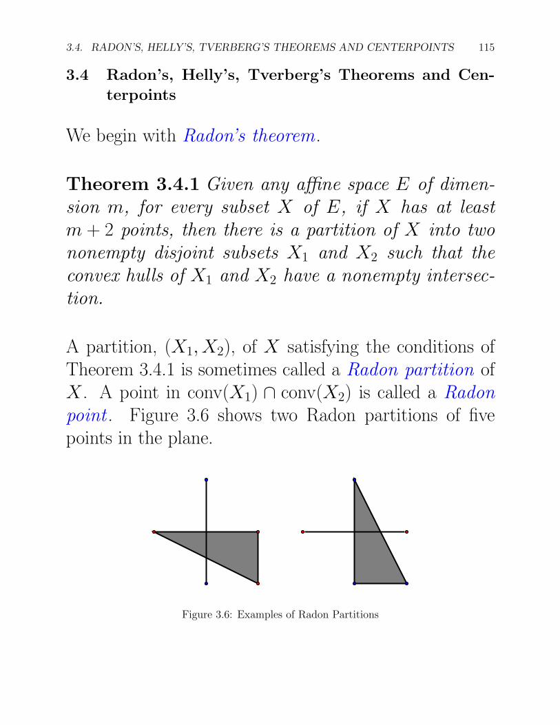
3.4. RADON’S, HELLY’S, TVERBERG’S THEOREMS AND CENTERPOINTS 115

3.4 Radon’s, Helly’s, Tverberg’s Theorems and Cen-

terpoints

We begin with Radon’s theorem.

Theorem 3.4.1 Given any affine space E of dimen-sion m, for every subset X of E, if X has at leastm + 2 points, then there is a partition of X into twononempty disjoint subsets X1 and X2 such that theconvex hulls of X1 and X2 have a nonempty intersec-tion.

A partition, (X1, X2), of X satisfying the conditions ofTheorem 3.4.1 is sometimes called a Radon partition ofX . A point in conv(X1) ∩ conv(X2) is called a Radonpoint . Figure 3.6 shows two Radon partitions of fivepoints in the plane.

Figure 3.6: Examples of Radon Partitions


Figure 3.7: The Radon Partitions of four points (in A2)

It can be shown that a finite set, X ⊆ E, has a uniqueRadon partition iff it has m + 2 elements and any m + 1points of X are affinely independent.

For example, there are exactly two possible cases in theplane as shown in Figure 3.7.

There is also a version of Radon’s theorem for the classof cones with an apex.

Say that a convex cone, C ⊆ E, has an apex (or is apointed cone) iff there is some hyperplane, H , such thatC ⊆ H+ and H ∩ C = {0}.

For example, the cone obtained as the intersection of twohalf spaces in R

3 is not pointed since it is a wedge with aline as part of its boundary.


Theorem 3.4.2 Given any vector space E of dimen-sion m, for every subset X of E, if cone(X) is apointed cone such that X has at least m + 1 nonzerovectors, then there is a partition of X into two nonemptydisjoint subsets, X1 and X2, such that the cones,cone(X1) and cone(X2), have a nonempty intersectionnot reduced to {0}.

There is a beautiful generalization of Radon’s theoremknown as Tverberg’s Theorem.

Theorem 3.4.3 (Tverberg’s Theorem, 1966) Let Ebe any affine space of dimension m. For any naturalnumber, r ≥ 2, for every subset, X, of E, if X has atleast (m+1)(r−1)+1 points, then there is a partition,(X1, . . . , Xr), of X into r nonempty pairwise disjointsubsets so that

⋂ri=1 conv(Xi) = ∅.

A partition as in Theorem 3.4.3 is called a Tverberg par-tition and a point in

⋂ri=1 conv(Xi) is called a Tverberg

point .


Theorem 3.4.3 was conjectured by Birch and proved byTverberg in 1966. Tverberg’s original proof was techni-cally quite complicated. Tverberg then gave a simplerproof in 1981 and other simpler proofs were later given,notably by Sarkaria (1992) and Onn (1997), using theColorful Caratheodory theorem.

A proof along those lines can be found in Matousek [?],Chapter 8, Section 8.3. A colored Tverberg theorem andmore can also be found in Matousek [?] (Section 8.3).


Next, we state a version of Helly’s theorem.

Theorem 3.4.4 Given any affine space E of dimen-sion m, for every family {K1, . . . , Kn} of n convexsubsets of E, if n ≥ m+2 and the intersection

⋂i∈I Ki

of any m + 1 of the Ki is nonempty (where I ⊆{1, . . . , n}, |I| = m + 1), then

⋂ni=1 Ki is nonempty.

An amusing corollary of Helly’s theorem is the followingresult: Consider n ≥ 4 parallel line segments in the affineplane A

2. If every three of these line segments meet aline, then all of these line segments meet a common line.


Centerpoints generalize the notion of median to higherdimensions.

Recall that if we have a set of n data points,S = {a1, . . . , an}, on the real line, a median for S isa point, x, such that both intervals [x,∞) and (−∞, x]contain at least n/2 of the points in S (by n/2, we meanthe largest integer greater than or equal to n/2).

Definition 3.4.5 Let S = {a1, . . . , an} be a set of npoints in A

d. A point, c ∈ Ad, is a centerpoint of S iff

for every hyperplane, H , whenever the closed half-spaceH+ (resp. H−) contains c, then H+ (resp. H−) containsat least n

d+1 points from S (by nd+1, we mean the largest

integer greater than or equal to nd+1, namely the ceiling

� nd+1� of n

d+1).

So, for d = 2, for each line, D, if the closed half-planeD+ (resp. D−) contains c, then D+ (resp. D−) containsat least a third of the points from S.

For d = 3, for each plane, H , if the closed half-space H+

(resp. H−) contains c, then H+ (resp. H−) contains atleast a fourth of the points from S, etc.


Figure 3.8: Example of a centerpoint

Example 3.8 shows nine points in the plane and one oftheir centerpoints (in red). This example shows that thebound 1

3 is tight.

Observe that a point, c ∈ Ad, is a centerpoint of S iff

c belongs to every open half-space,◦

H+ (resp.◦

H−) con-taining at least dn

d+1 + 1 points from S (again, we mean

� dnd+1� + 1).

We are now ready to prove the existence of centerpoints.


Theorem 3.4.6 Every finite set, S = {a1, . . . , an}, ofn points in A

d has some centerpoint.

The proof is by induction and its uses the second charac-terization of centerpoints involving open half-spaces con-taining at least dn

d+1 + 1 points.

The proof actually shows that the set of centerpoints ofS is a convex set.

It should also be noted that Theorem 3.4.6 can be provedeasily using Tverberg’s theorem (Theorem 3.4.3). Indeed,for a judicious choice of r, any Tverberg point is a cen-terpoint!

In fact, it is a finite intersection of convex hulls of finitelymany points, so it is the convex hull of finitely manypoints, in other words, a polytope.


Jadhav and Mukhopadhyay have given a linear-time algo-rithm for computing a centerpoint of a finite set of pointsin the plane.

For d ≥ 3, it appears that the best that can be done(using linear programming) is O(nd).

However, there are good approximation algorithms (Clark-son, Eppstein, Miller, Sturtivant and Teng) and in E

3

there is a near quadratic algorithm (Agarwal, Sharir andWelzl).

Miller and Sheehy (2009) have given an algorithm for find-ing an approximate centerpoint in sub-exponential timetogether with a polynomial-checkable proof of the approx-imation guarantee.


Chapter 4

Separation and SupportingHyperplanes

4.1 Separation Theorems and Farkas Lemma

It seems intuitively rather obvious that if A and B aretwo nonempty disjoint convex sets in A

2, then there isa line, H , separating them, in the sense that A and Bbelong to the two (disjoint) open half–planes determinedby H .

However, this is not always true! For example, this failsif both A and B are closed and unbounded (find an ex-ample).

Nevertheless, the result is true if both A and B are open,or if the notion of separation is weakened a little bit.

125

126 CHAPTER 4. SEPARATION AND SUPPORTING HYPERPLANES

The key result, from which most separation results follow,is a geometric version of the Hahn-Banach theorem.

In the sequel, we restrict our attention to real affine spacesof finite dimension. Then, if X is an affine space of di-mension d, there is an affine bijection f between X andA

d.

Now, Ad is a topological space, under the usual topology

on Rd (in fact, A

d is a metric space).

Recall that if a = (a1, . . . , ad) and b = (b1, . . . , bd)are any two points in A

d, their Euclidean distance,d(a, b), is given by

d(a, b) =√

(b1 − a1)2 + · · · + (bd − ad)2,

which is also the norm, ‖ab‖, of the vector ab and thatfor any ε > 0, the open ball of center a and radius ε,B(a, ε), is given by

B(a, ε) = {b ∈ Ad | d(a, b) < ε}.

4.1. SEPARATION THEOREMS AND FARKAS LEMMA 127

A subset U ⊆ Ad is open (in the norm topology) if

either U is empty or for every point, a ∈ U , there issome (small) open ball, B(a, ε), contained in U .

A subset C ⊆ Ad is closed iff A

d − C is open. Forexample, the closed balls , B(a, ε), where

B(a, ε) = {b ∈ Ad | d(a, b) ≤ ε},

are closed.

A subset W ⊆ Ad is bounded iff there is some ball (open

or closed), B, so that W ⊆ B.

A subset W ⊆ Ad is compact iff every family, {Ui}i∈I ,

that is an open cover of W (which means thatW =

⋃i∈I(W∩Ui), with each Ui an open set) possesses a

finite subcover (which means that there is a finite subset,F ⊆ I , so that W =

⋃i∈F (W ∩ Ui)).

In Ad, it can be shown that a subset W is compact iff W

is closed and bounded.


Given a function, f : Am → An, we say that f is con-

tinuous if f−1(V ) is open in Am whenever V is open in

An.

If f : Am → An is a continuous function, although it is

generally false that f (U) is open if U ⊆ Am is open,

it is easily checked that f (K) is compact if K ⊆ Am is

compact.

An affine space X of dimension d becomes a topologicalspace if we give it the topology for which the open subsetsare of the form f−1(U), where U is any open subset ofA

d and f : X → Ad is an affine bijection.

Given any subset, A, of a topological space X , the small-est closed set containing A is denoted by A, and is calledthe closure or adherence of A.

A subset, A, of X , is dense in X if A = X .

The largest open set contained in A is denoted by◦A, and

is called the interior of A.


x y

u

v

z

UV

W

Figure 4.1: Illustration for the proof of Lemma 4.1.1

The set Fr A = A ∩ X − A, is called the boundary (orfrontier ) of A. We also denote the boundary of A by∂A.

In order to prove the Hahn-Banach theorem, we will needtwo lemmas.

Given any two distinct points x, y ∈ X , we let

]x, y[ = {(1 − λ)x + λy ∈ X | 0 < λ < 1}.

Lemma 4.1.1 Let S be a nonempty convex set, and

let x ∈◦S and y ∈ S. Then, we have ]x, y[ ⊆ S.

Corollary 4.1.2 If S is convex, then◦S is also convex

and we have◦S =

◦S. Further, if

◦S = ∅, then S =

◦S.


Beware that if S is a closed set, then its convex hull,conv(S), is not necessarily closed! However, conv(S) isclosed when S is compact (see Proposition 3.2.3).

There is a simple criterion to test whether a convex sethas an empty interior, based on the notion of dimensionof a convex set.

Proposition 4.1.3 A nonempty convex set S has anonempty interior iff dim S = dim X.

� Proposition 4.1.3 is false in infinite dimension.

Proposition 4.1.4 If S is convex, then S is also con-vex.

One can also easily prove that convexity is preserved un-der direct image and inverse image by an affine map.


The next lemma, which seems intuitively obvious, is thecore of the proof of the Hahn-Banach theorem. This isthe case where the affine space has dimension two.

First, we need to define what is a convex cone with vertexx.

Definition 4.1.5 A convex set, C, is a convex conewith vertex x if C is invariant under all central magnifi-cations Hx,λ of center x and ratio λ, with λ > 0(i.e., Hx,λ(C) = C).

Given a convex set, S, and a point x /∈ S, we can define

conex(S) =⋃λ>0

Hx,λ(S).

It is easy to check that this is a convex cone with vertexx.

Lemma 4.1.6 Let B be a nonempty open and convexsubset of A

2, and let O be a point of A2 so that

O /∈ B. Then, there is some line, L, through O, sothat L ∩ B = ∅.


B

O

C

xL

Figure 4.2: Hahn-Banach Theorem in the plane (Lemma 4.1.6)

Finally, we come to the Hahn-Banach theorem.

Theorem 4.1.7 (Hahn-Banach theorem, geometricform) Let X be a (finite-dimensional) affine space, Abe a nonempty open and convex subset of X and L bean affine subspace of X so that A∩L = ∅. Then, thereis some hyperplane, H, containing L, that is disjointfrom A.

Proof . The case where dim X = 1 is trivial. Thus, wemay assume that dimX ≥ 2. We reduce the proof to thecase where dim X = 2.

Remark: The geometric form of the Hahn-Banach the-orem also holds when the dimension of X is infinite,but a more sophisticated proof is required (it uses Zorn’slemma).


A

L

H

Figure 4.3: Hahn-Banach Theorem, geometric form (Theorem 4.1.7)

� Theorem 4.1.7 is false if we omit the assumption thatA is open. For a counter-example, let A ⊆ A

2 be theunion of the half space y < 0 with the close segment[0, 1] on the x-axis and let L be the point (2, 0) on theboundary of A. It is also false if A is closed! (Find acounter-example).


A

L

H

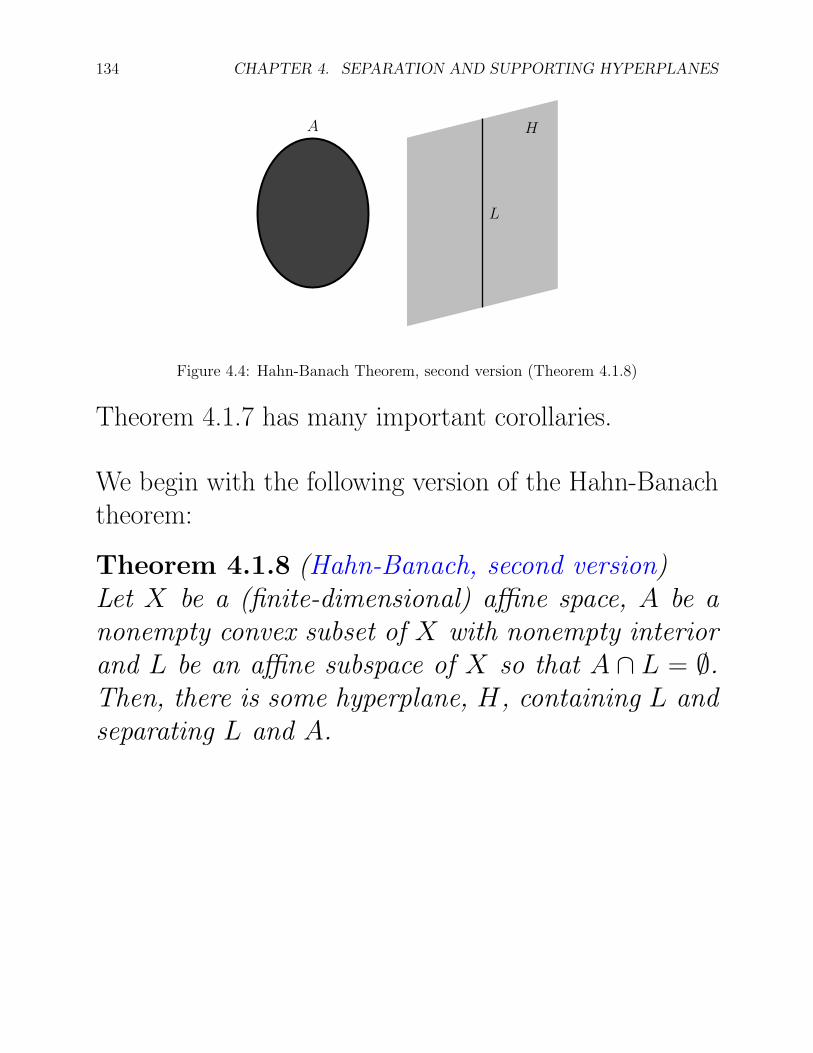
Figure 4.4: Hahn-Banach Theorem, second version (Theorem 4.1.8)

Theorem 4.1.7 has many important corollaries.

We begin with the following version of the Hahn-Banachtheorem:

Theorem 4.1.8 (Hahn-Banach, second version)Let X be a (finite-dimensional) affine space, A be anonempty convex subset of X with nonempty interiorand L be an affine subspace of X so that A ∩ L = ∅.Then, there is some hyperplane, H, containing L andseparating L and A.


A

B

H

Figure 4.5: Separation Theorem, version 1 (Corollary 4.1.9)

Corollary 4.1.9 Given an affine space, X, let A andB be two nonempty disjoint convex subsets and as-

sume that A has nonempty interior (◦A = ∅). Then,

there is a hyperplane separating A and B.

Remark: Theorem 4.1.8 and Corollary 4.1.9 also hold

in the infinite case.

Corollary 4.1.10 Given an affine space, X, let Aand B be two nonempty disjoint open and convex sub-sets. Then, there is a hyperplane strictly separatingA and B.


Beware that Corollary 4.1.10 fails for closed convex sets.However, Corollary 4.1.10 holds if we also assume that A(or B) is compact.

We need to review the notion of distance from a pointto a subset .

Let X be a metric space with distance function d. Givenany point a ∈ X and any nonempty subset B of X , welet

d(a, B) = infb∈B

d(a, b)

(where inf is the notation for least upper bound).

Now, if X is an affine space of dimension d, it can begiven a metric structure by giving the corresponding vec-tor space a metric structure, for instance, the metric in-duced by a Euclidean structure.

We have the following important property: For anynonempty closed subset, S ⊆ X (not necessarily con-vex), and any point, a ∈ X , there is some point s ∈ S“achieving the distance from a to S,” i.e., so that

d(a, S) = d(a, s).


Corollary 4.1.11 Given an affine space, X, let Aand B be two nonempty disjoint closed and convexsubsets, with A compact. Then, there is a hyperplanestrictly separating A and B.

A “cute” application of Corollary 4.1.11 is one of themany versions of “Farkas Lemma” (1893-1894, 1902), abasic result in the theory of linear programming.

For any vector, x = (x1, . . . , xn) ∈ Rn, and any real,

α ∈ R, write x ≥ α iff xi ≥ α, for i = 1, . . . , n.


Lemma 4.1.12 (Farkas Lemma, Version I) Given anyd × n real matrix, A, and any vector, z ∈ R

d, exactlyone of the following alternatives occurs:

(a) The linear system, Ax = z, has a solution, x =(x1, . . . , xn), such that x ≥ 0 and x1 + · · ·+xn = 1,or

(b) There is some c ∈ Rd and some α ∈ R such that

c�z < α and c�A ≥ α.

Remark: If we relax the requirements on solutions ofAx = z and only require x ≥ 0 (x1 + · · · + xn = 1 isno longer required) then, in condition (b), we can takeα = 0. This is another version of Farkas Lemma.

In this case, instead of considering the convex hull of{A1, . . . , An} we are considering the convex cone,

cone(A1, . . . , An) =

{λA1 + · · · + λnAn | λi ≥ 0, 1 ≤ i ≤ n},that is, we are dropping the condition λ1 + · · ·+ λn = 1.For this version of Farkas Lemma we need the followingseparation lemma:


H ′ H

aO C

Figure 4.6: Illustration for the proof of Proposition 4.1.13

Proposition 4.1.13 Let C ⊆ Ed be any closed convex

cone with vertex O. Then, for every point, a, notin C, there is a hyperplane, H, passing through Oseparating a and C with a /∈ H.

Lemma 4.1.14 (Farkas Lemma, Version II) Givenany d × n real matrix, A, and any vector, z ∈ R

d,exactly one of the following alternatives occurs:

(a) The linear system, Ax = z, has a solution, x, suchthat x ≥ 0, or

(b) There is some c ∈ Rd such that c�z < 0 and

c�A ≥ 0.

One can show that Farkas II implies Farkas I.


Here is another version of Farkas Lemma having to dowith a system of inequalities, Ax ≤ z. Although, thisversion may seem weaker that Farkas II, it is actuallyequivalent to it!

Lemma 4.1.15 (Farkas Lemma, Version III) Givenany d × n real matrix, A, and any vector, z ∈ R

d,exactly one of the following alternatives occurs:

(a) The system of inequalities, Ax ≤ z, has a solution,x, or

(b) There is some c ∈ Rd such that c ≥ 0, c�z < 0

and c�A = 0.

The proof uses two tricks from linear programming:

1. We convert the system of inequalities, Ax ≤ z, into asystem of equations by introducing a vector of slackvariables , γ = (γ1, . . . , γd), where the system of equa-tions is

(A, I)

(xγ

)= z,

with γ ≥ 0.

2. We replace each “unconstrained variable”, xi, byxi = Xi − Yi, with Xi, Yi ≥ 0.


Then, the original system Ax ≤ z has a solution, x (un-constrained), iff the system of equations

(A,−A, I)

(XYγ

)= z

has a solution with X,Y, γ ≥ 0.

By Farkas II, this system has no solution iff there existssome c ∈ R

d with c�z < 0 and

c�(A,−A, I) ≥ 0,

that is, c�A ≥ 0, −c�A ≥ 0, and c ≥ 0.

However, these four conditions reduce to c�z < 0,c�A = 0 and c ≥ 0.


x

−x

A

B

A + x

C

A − x

D

H

O

Figure 4.7: Separation Theorem, final version (Theorem 4.1.16)

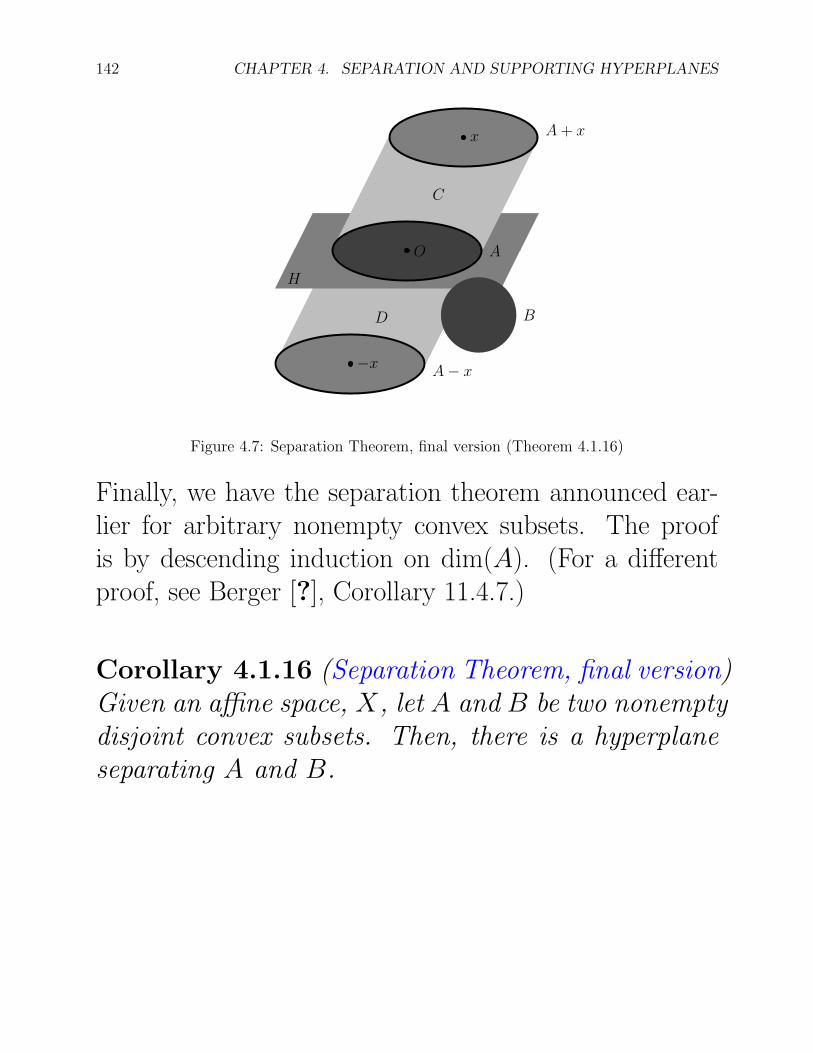
Finally, we have the separation theorem announced ear-lier for arbitrary nonempty convex subsets. The proofis by descending induction on dim(A). (For a differentproof, see Berger [?], Corollary 11.4.7.)

Corollary 4.1.16 (Separation Theorem, final version)Given an affine space, X, let A and B be two nonemptydisjoint convex subsets. Then, there is a hyperplaneseparating A and B.


Remarks:

(1) The reader should compare the proof from Valentine[?], Chapter II with Berger’s proof using compactnessof the projective space P

d [?] (Corollary 11.4.7).

(2) Rather than using the Hahn-Banach theorem to de-duce separation results, one may proceed differentlyand use the following intuitively obvious lemma, as inValentine [?] (Theorem 2.4):

Lemma 4.1.17 If A and B are two nonempty con-vex sets such that A∪B = X and A∩B = ∅, thenV = A ∩ B is a hyperplane.

One can then deduce Corollaries 4.1.9 and 4.1.16. Yetanother approach is followed in Barvinok [?].

(3) How can some of the above results be generalized toinfinite dimensional affine spaces, especially Theorem4.1.7 and Corollary 4.1.9?


One approach is to simultaneously relax the notionof interior and tighten a little the notion of closure,in a more “linear and less topological” fashion, as inValentine [?].

Given any subset A ⊆ X (where X may be infi-nite dimensional, but is a Hausdorff topological vectorspace), say that a point x ∈ X is linearly accessi-ble from A iff there is some a ∈ A with a = x and]a, x[ ⊆ A. We let lina A be the set of all pointslinearly accessible from A and lin A = A ∪ lina A.

A point a ∈ A is a core point of A iff for everyy ∈ X , with y = a, there is some z ∈]a, y[ , suchthat [a, z] ⊆ A. The set of all core points is denotedcore A.

It is not difficult to prove that lin A ⊆ A and◦A ⊆ core A. If A has nonempty interior, then

lin A = A and◦A = core A.


Also, if A is convex, then core A and lin A are con-vex. Then, Lemma 4.1.17 still holds (where X is notnecessarily finite dimensional) if we redefine V asV = lin A ∩ lin B and allow the possibility that Vcould be X itself.

Corollary 4.1.9 also holds in the general case if we as-sume that core A is nonempty. For details, see Valen-tine [?], Chapter I and II.

(4) Yet another approach is to define the notion of analgebraically open convex set, as in Barvinok [?].

A convex set, A, is algebraically open iff the inter-section of A with every line, L, is an open interval,possibly empty or infinite at either end (or all of L).

An open convex set is algebraically open. Then, theHahn-Banach theorem holds provided that A is analgebraically open convex set and similarly, Corollary4.1.9 also holds provided A is algebraically open.

For details, see Barvinok [?], Chapter 2 and 3. We donot know how the notion “algebraically open” relatesto the concept of core.


(5) Theorems 4.1.7, 4.1.8 and Corollary 4.1.9 are provedin Lax using the notion of gauge function in the moregeneral case where A has some core point (but bewarethat Lax uses the terminology interior point insteadof core point!).

An important special case of separation is the case whereA is convex and B = {a} for some point a in A.

4.2. SUPPORTING HYPERPLANES AND MINKOWSKI’S PROPOSITION 147

4.2 Supporting Hyperplanes and Minkowski’s Propo-

sition

Recall the definition of a supporting hyperplane given inDefinition 3.3.2. We have the following important propo-sition first proved by Minkowski (1896):

Proposition 4.2.1 (Minkowski) Let A be a nonemptyclosed and convex subset. Then, for every point,a ∈ ∂A, there is a supporting hyperplane to A througha.

� Beware that Proposition 4.2.1 is false when the dimen-

sion X of A is infinite and when◦A = ∅.

The proposition below gives a sufficient condition for aclosed subset to be convex.

Proposition 4.2.2 Let A be a closed subset withnonempty interior. If there is a supporting hyperplanefor every point a ∈ ∂A, then A is convex.

� The condition that A has nonempty interior is crucial!


The proposition below characterizes closed convex sets interms of (closed) half–spaces. It is another intuitive factwhose rigorous proof is nontrivial.

Proposition 4.2.3 Let A be a nonempty closed andconvex subset. Then, A is the intersection of all theclosed half–spaces containing it.

Documents

Chapter 3 Basic Properties of Convex Setscis610/convex1-09.pdf3.1. CONVEX SETS 95 It is obvious that the intersection of any family (ﬁnite or inﬁnite) of convex sets is convex