CHAPTER 3 BACKGROUND AND RELATED WORK · CHAPTER 3 BACKGROUND AND RELATED WORK This chapter will provide the background knowledge required for the rest of this thesis. It will start

CHAPTER 3

BACKGROUND AND RELATED WORK

This chapter will provide the background knowledge required for the rest of this thesis. It will

start with the definition of the input signal function and terminology related to the

triangulation mesh. This will be followed by a discussion of the triangular representation, the

image reconstruction method and its error metric. The definitions of Delaunay and data

dependent triangulation will also be presented in this chapter. Finally, this chapter will end

with a discussion of graph theory for triangular mesh applications.

3.1 Input and Output Data

Usually a natural gray-scale image contains a lot of redundant information. This redundancy

in data can be used for file compression so that less storage or transfer capacity will be

required. The similarity in intensity and rate of change at different scales are some of the

duplications in data that can be used in compression. Since it is possible to segment some

regions into triangles without substantially degrading the quality of the image, a triangular

mesh is a good approach for data compression for storage reduction and data processing.

3.1.1 Gray-Scale Image

A gray-scale image is usually presented in the two-dimensional domain. It can be viewed as a

set of finite intensity (or magnitude) values being sampled at finite intervals with time (or

space) domain. This can be mathematically expressed as:

( ) 1| , , 1,..., , 1,...,ij ij i jV v v f x y i N j N= = ∈Ω = = 2 (3.1)

where represents the parameter domain and and represent the number of samples

along each dimension of the image. Meanwhile, the intensity of the image, which can be

found at each of the sample points, can be defined as:

Ω 1N 2N

22

CHAPTER 3. BACKGROUND AND RELATED WORK

( ),i j if x y z= j N

)

)

y

, and (3.2) 11,...,i N= 21,...,j =

where represents the quantized value of the intensity at sample location ( . Normally

this value is in an integer that ranges from 0 to 255.

ijz ,i jx y

3.1.2 Triangulation

A triangulation is a partitioning of the 2D image plane into a set of triangles. It may be

represented using a set of appropriate vertices, which are located on the original grid of

sample points, and a set of edges that connects those vertices. A vertex can be represented by

three parameter variables as

( )1 1 1, ,i i i iV x y I= (3.3) 1 2 31 Vi i i N≤ ≠ ≠ ≤

where is the number of vertices found in the triangulation. Note that ( is the

sampled location of the vertex V and is the quantized intensity at that location.

VN1 2,i ix y

i iI

In addition to vertex information, a triangulation requires vertex connection

information. This relationship is usually defined in the form of edges. An edge is a line

segment that connects two vertices and it can be expressed by

( )1 2,i i iE V V= , (3.5) 1 21 Ei i N≤ ≠ ≤

A triangle is a planar patch, which is determined by three non-collinear points that are

connected by three line segments. This patch can be defined by

( )1 2 3, ,i i i iT V V V= , (3.4) 1 2 31 Ti i i N≤ ≠ ≠ ≤

where the three vertices V ,V and V are located at three different sample points in the two-

dimensional plane and is the number of triangles. The triangulation, , in a finite

parametric domain, Ω⊂ , must satisfy four conditions:

i

2R

j k

x − TN VΓ

(i) Let V be the set of all vertices found in such that V V . VΓ i j φ=∩

(ii) j is either iE E∩ φ or a vertex if i j . ≠

(iii) , where is the number of triangles in a given triangulation. 1

TN

ii

T=

Ω = ∪ TN

(iv) is either iT T∩ j φ or a common edge , or a common vertex V if . kE k i j≠

23


Therefore the triangulation can be defined as VΓ

| 1,...,V i TT i NΓ = = (3.6)

Since it is common to define an operator for the number of elements in a set as i , we define

TN = ΓV as the number of triangles in the triangulation , which covers the parameter

domain and

VΓ

2RΩ⊂ VN V= as the number of vertices in the triangulation . VΓ

Figure 3.1 and 3.2 illustrate some of the regular sampled grid triangulations and how

the sampling can affect the quality of the image. The original image of a crater lake is shown

in Figure 3.1 (a) while (b) shows an example of the locations of points on the 16x16 regular

sample grid. Figure 3.2 (a-c) show the triangulations that are sampled at different regular

finite intervals of 4, 8 and 16 respectively. Since the image size is 256x256, the grid sizes are

64x64, 32x32 and 16x16 respectively while the reconstructed images are shown in Figure 3.2

(d-f). These images are reconstructed using the Gouraud shading technique, which will be

explained in Section 3.3. Although denser triangulation gives a better approximation of

the original image, it requires more vertices and triangles for image representation.

VΓ

3.2 Delaunay and Data-Dependent Triangulations

There has been much research concerning the minimization of error using refinement

methods. Some of these methods are greedy insertion [De Floriani et al. 85], feature-based

[Scarlatos and Pavlidis 92], and hierarchical subdivision [De Floriani et al. 84]. The greedy

insertion algorithm scans for a vertex location where total error reduction is achieved. This

method produces a good approximation of the original dataset. However it is time-consuming

to search for an optimal point. This drawback motivates the search for a faster algorithm. A

feature-based method is proposed using the features to determine the vertices or edges of the

triangulation [Chen and Schmitt 93]. Edge detectors and Laplacian filters have been proposed

to detect some of these features for vertex insertion in mesh refinement [Southard 91].

24


(a) (b)

Figure 3.1 – Regular sample grid. (a) Original image of crater lake of size 256x256. (b) Locations of sample points taken by the regular sampling grid of size 16x16.

(a) (b) (c)

(d) (e) (f)

Figure 3.2 - Approximation of an image using a regularly sampled triangular mesh. Triangular meshes with regular sampling grid size of (a) 64x64, (b) 32x32 and (c) 16x16. Reconstructed images using Gouraud shading on the regular sampling grid of (d) 64x64, (e) 32x32 and (f) 16x16 respectively.

Another approach is hierarchical subdivision [Scarlatos and Pavlidis 92], which

recursively subdivides a triangle into smaller sub-triangles to represent a better

approximation of the original dataset. The advantage of this method is its fast computation

and use of multiresolution modeling. Its reconstructed image quality, however, is no better

than that of the greedy insertion method.

Besides these refinement processes, one of the equally important decisions for triangle

representation is to determine the choice of triangles without considering error metrics. One

of the proposed methods for choosing triangles is Delaunay triangulation [Kropatsch and

Bischof 01]. Generally, this type of triangulation is known as the dual of the Voronoi

25


diagram, which segments the parameter domain into regions in such a way that points lying

in the same region are located nearest to the vertex of its region. A Voronoi polygon is

defined by

( ) ( ,i ii j

p H p pκ≠∩ )j

)

(3.7)

where is a discrete point (or vertex) of interest and is a half-plane that contains

the set of points that lie in and are located nearer to than to . Therefore, if there are

vertices in the domain, each Voronoi polygon can result from the intersection of at most

half-planes. These polygons are convex with no more than sides.

ip ( ,i jH p p

ip2R jp

N −

N

N 1− 1

Delaunay triangulation can be achieved from a Voronoi diagram by connecting

vertices, whose regions in the Voronoi diagram intersect. The result of using the Delaunay

scheme is the triangulation that maximizes the minimum angles of all triangles. In other

words, in a Delaunay triangulation, the circle that circumscribes three vertices of any triangle

contains no other vertices. Figure 3.3 below shows an example of a Voronoi diagram with ten

vertices of interest and its corresponding Delaunay triangulations, while Figure 3.4 shows an

example of Delaunay triangulation and non-Delaunay triangulation.

Figure 3.3 - Example of a Voronoi diagram and its Delaunay triangulation. (a) Voronoi diagram and its points (or vertices) of interest. (b) Corresponding Delaunay triangulation.

26


Figure 3.4 – Concept of Delaunay triangulation. (a) In a Delaunay triangulation, no other vertices lie in the circumscribing circle of each triangle. Circle C does not include vertex V and circle C does not contain vertex V . (b) Non-Delaunay triangulation. Circle C contains more than three vertices. It includes vertices V , V , V and V .

1 4

2 1 1

1 2 3 4

Although the Delaunay triangulation method is fast in regularizing the triangulation, it

does not guarantee an optimal solution to the approximation. In many applications, the choice

of Delaunay triangulation can significantly increase the approximation error. It is found that

non-Delaunay triangles can produce a better result in most cases because long, sliver triangles

can give a better approximation, especially along the edges, where large changes in intensity

occur.

Figure 3.5 compares the results of reconstructed images of Lena using both Delaunay

triangulation and non-Delaunay triangulation. An edge swap operation, which will be

discussed in Section 5.4.1, is performed on the 16x16 regular grid triangulation to improve

the reconstruction image quality. It can be observed that the Delaunay triangulation tends to

produce a lot of inappropriate triangles along the edge in the image. This is because it does

not allow the thin, sliver triangles in the set. However, the data-dependent triangulation,

which permits sliver triangles, yields a better rough approximation to the image data. The

reason is that a change in intensity can be represented more accurately by thin, sliver triangles

by short, ‘fat’ triangles. However it is possible to combine these two important parameters to

achieve a better result. The choice of combining Delaunay and data-dependent triangles will

be discussed in Section 5.4.1.

27


(a)

(b) (c)

(d) (e)

Figure 3.5 – Comparison of Delaunay triangulation and non-Delaunay triangulation. (a) Original image of Lena. (b-c) A Delaunay triangulation and its reconstructed image. (d-e) A non-Delaunay triangulation and its reconstructed image.

28


3.3 Gouraud Shading

There are many techniques to perform shading of a triangle. The choice of rendering not only

helps the triangulation-based image look more realistic, but also smooths the edges between

adjacent triangles. The shading technique used in this thesis is based on the Gouraud shading

technique [Watt 93]. Given a sequence of three vertices (V ,V and V ) and their intensity

values ( , and ), it is possible to perform Gouraud shading on a triangle by bilinear

interpolation. Figure 3.6 shows the concept of how Gouraud shading can be performed.

1 2 3

1I 2I 3I

To render a triangle, first, its maximum and minimum values ( and ) in the

(vertical) direction are determined. These two values are used for the vertical scan

limitation. Next, for each row starting from to , its horizontal boundaries (

and ) and their intensities ( and ) are calculated by interpolating a necessary pair of

vertices, whose edges give the limitation of the horizontal boundaries.

maxy miny

y

sy

aI

maxy miny ax

bx bI

( ) ( )( )

2 11

2 1a s

x xx y y

y y−

= − +− 1x (3.8)

( ) ( )( )

3 11

3 1b s

x xx y y

y y−

= − +− 1x (3.9)

( ) ( )( )

2 11

2 1a s

I II y y

y y−

= − +− 1I (3.10)

( ) ( )( )

3 11

3 1b s

I II y y

y y−

= − +− 1I (3.11)

These interpolated values not only smooth the intensity between two vertex points but also

smooth the connection between two connected triangles. This is because the two connected

triangles share the two vertices of same location and intensity. Finally, in the same way, the

intensity inside the triangle can be calculated by the horizontal scan of . With each value of

from to , the intensity inside the triangle, , can be calculated as

sx

sx ax bx sI

( ) ( )( )

b as s a

b a

I II x x

x x−

= − +− aI (3.12)

29


( )2 2 2 2, ,V x y I y

Vertical Scan of sy

( )1 1 1 1, ,x y I

( )1 , ,c c cV x y I

maxy

Figure 3

For com

where

method

addition

error ten

∆

O

as Mach

brighter

system

93]. Fig

perceive

x

.6 – Gouraud shading

putational efficiency,

is the incremente

significantly improve

. However one of its d

ds to get larger as n in

sI

ne of the disadvantag

banding. The chang

or darker band of in

to the first derivative

ure 3.7 shows the Mac

d signal relative to th

( ), ,a s ax y I

miny

– bilinear intensity inter

incremental calculation

( ) ( )s bb a

xI Ix x∆

∆ = −− aI

I, , 1s n s n sI I −= + ∆

d change in intensity a

s the calculation time by

rawbacks is its imprecis

creases.

es of employing Gourau

e in intensity triggers t

tensity. This is due to th

of intensity, which is u

h band phenomenon. N

e actual ramp signal.

30

( ), ,b s bx y I

V

( )3 3 3 3, ,x y I

polatio

is pref

nd n i

repla

ion. Si

d shad

he hum

e high

sed to

otice th

V

n.

erable:

(3.13)

(3.14)

s the value from to . This

cing multiplication operator with

nce there is round off in , the

ax bx

I∆ s

ing is a visual side effect known

an visual system to perceive a

sensitivity in the human visual

detect and enhance edges [Watt

e overshoot that occurring in the


Figure 3.7 – Mach band phenomenon. (a) Actual signal intensity. (b) Signal intensity perceived by human visual system.

3.4 Error Metric

Since a reconstructed image is an approximation of the original, there will be an error

between the original and the reconstruction. Therefore it is necessary to define an error metric

to measure the quality of the reconstructed image. Let be a planar patch that approximates

a triangular region, , in an image. For i , must satisfy a plane equation

defined by ich can be determined by the three vertices forming

the triangle T . In the parameter domain, this approximated patch can be defined as:

iTf

TiT

i i

1,2,...,= NiTf

( ), iP x y a x b y c= + + ,

i

i wh

) )

)

( ,iTf x y = (3.15) ( ),

0iP x y ( ) (, ix y T

otherwise∈Ω

( ,iP x y , = (3.16) ( )ig z 1 2 3, ,i i i i=

where defined the boundary of the parameter domain of the triangulations and i ,

and are the vertices of triangle . The function is used for a better approximation

when noise or a high frequency component is present in the data. Since the wavelet transform

yields both approximation and detail of the original data, the function can take

( )iTΩ 1 2i

3i iT ( )g z

( )g z

31


advantage of this computation. With the definition of the approximation of triangles, the

approximation of the triangulation can be defined as

∑=

Γ =∧

t

iTi

V

ff1

(3.17)

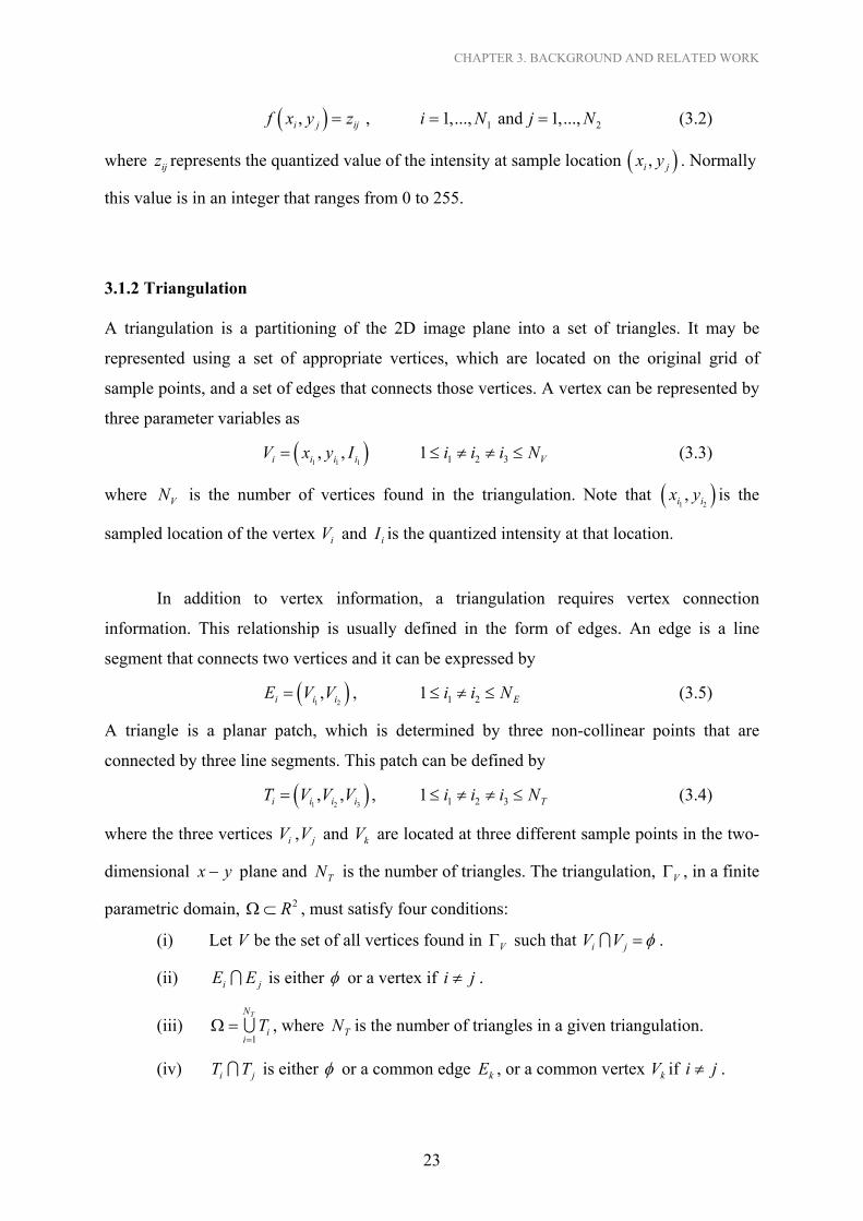
which accounts for the approximation of non-overlapping triangles. The error metric,

which is shown in Figure 3.8, can be denoted by

TN

V

f f∧Γ

− . It is normally measured by the

average of the sum of squared errors, which is normally called mean-squared error (MSE).

MSE can be defined as

( ) ( )2

2 1 , ,vy x

f x y f x y dxdyx y ∧Γ

∆ ∆

∆ = −∆ ∆ ∫ ∫ (3.18)

This is computationally equivalent to

( ) ( )2

1 1

1 , ,V

M N

y x

MSE f x y f x yMN ∧Γ

= =

= − ∑∑ (3.19)

where M and N denote the height and width of the image respectively. Another popular error

metric is the peak-signal-to-noise ratio ( ). It is defined by PSNR

max1020log IPSNR

MSE= (3.20)

where is the possible maximum intensity value in of the image. Usually, this value is

255 for a gray-scale image. In reconstruction, a , that is larger than 30 dB, will often

appear to have little or no visible degradation. However this still depends on the image itself.

maxI

PSNR

3.5 Graph Theory

Since the approximation algorithm in this thesis is based on triangulation, the two-

dimensional image has to be segmented into many triangular regions, which are represented

by three vertices. One of the solutions to present this type of data structure is to use an

undirected graph. A graph G V consists of a set of vertices, V, and a set of edges, E,

which defines a relationship between the vertices.

( , E= )

32


Figure 3.8 – Error calculation

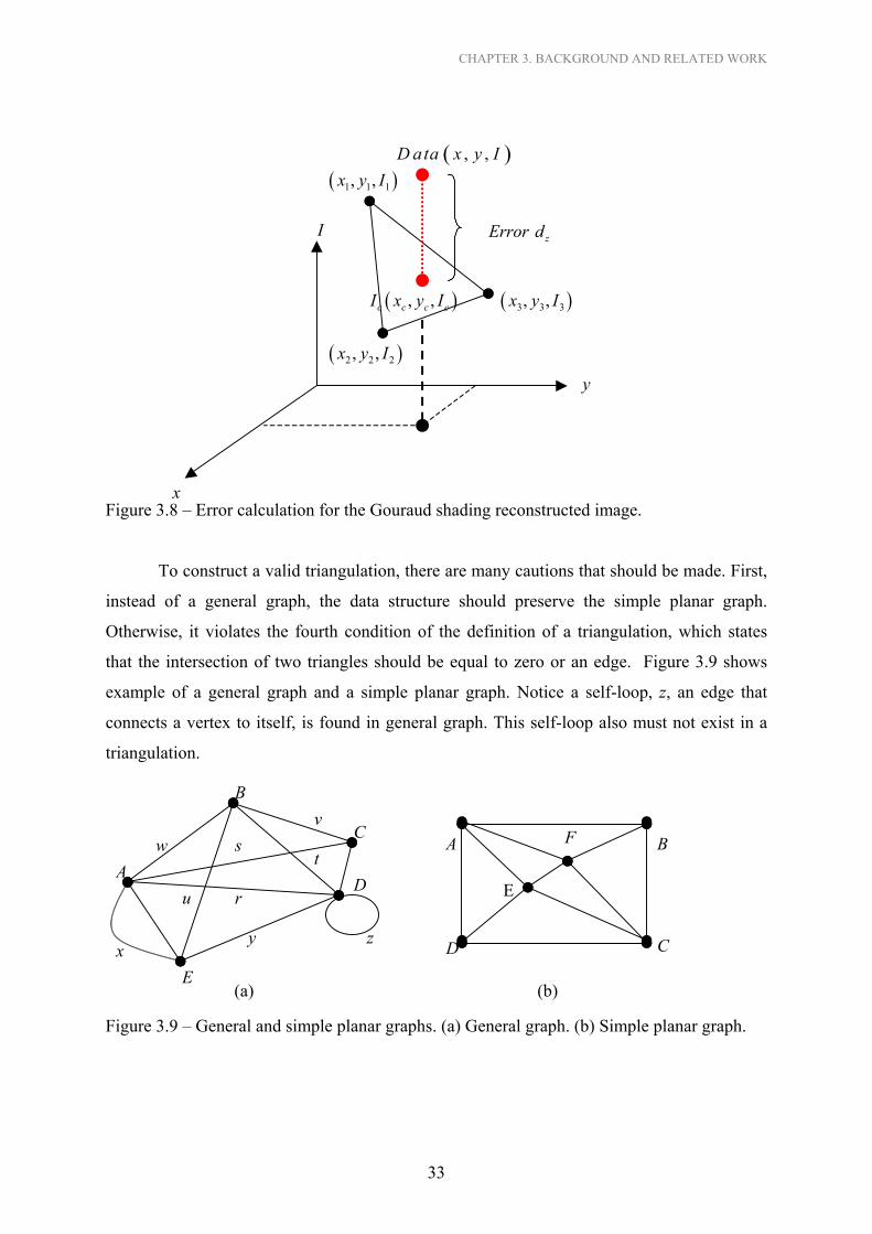
To construct a valid tri

instead of a general graph,

Otherwise, it violates the fou

that the intersection of two tri

example of a general graph a

connects a vertex to itself, is

triangulation.

w

x

B

y

v

u

ts

r

I

x

( )1 1 1, ,x y I( ), ,D ata x y I

A

E

(a)

Figure 3.9 – General and simp

for the

angul

the d

rth co

angle

nd a

found

C

D

( 2,x

( ), ,c c c cI x y I ( )3 3 3, ,x y I

Error zd

le pla

Go

atio

ata

ndit

s sh

sim

in

z

2,y I

nar

uraud shading

n, there are ma

structure shou

ion of the defi

ould be equal

ple planar grap

general graph.

)2

D

A

graphs. (a) Gen

33

y

reconstruct

ny cautions

ld preserve

nition of a

to zero or

h. Notice

This self-lo

E

F

(b)

eral graph.

ed image.

that should be made. First,

the simple planar graph.

triangulation, which states

an edge. Figure 3.9 shows

a self-loop, z, an edge that

op also must not exist in a

B

C

(b) Simple planar graph.


Since the graph is mathematically defined by its vertices and their binary relation, the

positions of the vertices and the curvature of the edge are not factors used to consider the

equivalence of the two graphs. Figure 3.10 shows two equivalent graphs, which have

different representations.

x w

A v B z

s

r

q

P

O

N

M

t

u C y D

(a) (b)

Figure 3.10 – Equivalent graphs. (a) Original graph. (b) Equivalent graph with different representation.

It is possible to show that these two graphs are equivalent by the bijection mapping of

the vertex and edge names. The following shows the equivalences to show that they are the

same graphs.

Edge Equivalent v q→

Two graphs G

such

bijection can be d

=

:f G G→

vf

Furthermore, the

isomorphic funct

by

Vertex Equivalent

w rx sy tz u

→→→→

A MB NC OD P

→→→→

V and G V are isomorphic if there exists at least one bijection

that ( ) if and only if . This vertex and edge

efined by:

( , E ) ))

G

( , E=

E∈,U V ( ) ( )( ,f U f V E∈

: G GV V→ and (3.21) :e Gf E E→

composite function f also inherits the isomorphism property from the two

ions. The composite functions of two isomorphic functions can be denoted

( )1 2 1 2f f f f f= = (3.22)

34


In the special case of a simple graph, if there exists a vertex bijection such that

is adjacent to if and only if x is adjacent to y for all ( ) , the two graphs

are isomorphic. Therefore only vertex bijection is sufficient to show isomorphism of the two

simple graphs. This property is essential to designing templates for initial triangulation,

which will be discussed in Section 4.2.3.

:v G Gf V V→

GV∈( )f x ( )f y ,x y

35

Documents

CHAPTER 3 BACKGROUND AND RELATED WORK · CHAPTER 3 BACKGROUND AND RELATED WORK This chapter will provide the background knowledge required for the rest of this thesis. It will start