Embed Size (px)
Citation preview

1
Chapter 26: Smith Charts
Chapter Learning Objectives: After completing this chapter the student will be able to:
Plot an impedance or admittance on a Smith chart.
Use a Smith chart to determine the input impedance of a terminated transmission line.
Use a Smith chart to design a single-stub tuner to match a load impedance to a transmission line’s characteristic impedance.
You can watch the video associated
with this chapter at the following link:
Historical Perspective: Phillip H. Smith (1905-1987) was a
an American electrical engineer who worked for Bell
Telephone Laboratories. He is best known for inventing the
Smith chart, which is a very useful graphical tool for working
with transmission lines and RF circuits.
Smith Chart image © 2015 IEEE. Used with permission.

2
Introduction to the Smith Chart
The Smith chart is a graphical method for solving problems involving transmission lines and
radio frequency (RF) loads such as antennas. It was invented in 1936, and for more than 50
years, it was the most important tool in the RF engineer’s toolkit. Since the 1980s, computer
tools have become much more powerful, and pencil-and-paper Smith charts are used less
frequently, but they are still incredibly useful for visualizing the problems associated with
transmission lines and loads. Many computer tools and digital measurement devices still use
Smith charts to convey information to their users.
Smith charts can be used to plot impedances, admittances, reflection coefficients, and many other
quantities that are beyond the scope of this discussion such as scattering parameters, noise
figures, and measures of stability.
We know that the impedance of a transmission line (the ratio of the voltage divided by the
current) varies from point to point along the line, and that the impedance repeats itself every
half-wavelength. We will take advantage of this repetition by plotting the impedance on a circle,
where the circumference represents a half wavelength. In that way, one revolution around the
circle will return you to the same point, and moving a half wavelength along the line will return
you to the same impedance.
In order to allow one chart to handle any possible transmission line, we will “normalize” all the
impedances in the system by dividing them by the characteristic impedance of the transmission
line, Zc. We will use a lower-case z to represent impedances that have been normalized in this
manner.
(Equation 26.1)
Since the load impedance can have both a real part (due to resistance) and an imaginary part (due
to capacitance and/or inductance), we can represent it as follows:
(Equation 26.2)
Normalizing both the real and imaginary components of the impedance gives:
(Equation 26.3)
Where the normalization is performed as indicated by Equation 26.1:
26.1

3
(Equation 26.4)
(Equation 26.5)
Recall from chapter 25 that we derived the following equation for the input impedance of a
transmission line:
(Copy of Equation 25.10)
If we normalize this equation by dividing by ZC and then divide both the numerator and
denominator by ZC to normalize the elements inside the fraction, we find:
(Equation 26.6)
Recalling from chapter 24 the expression for reflection coefficient in terms of impedances:
(Copy of Equation 24.25)
Since the load impedance can be complex, the reflection coefficient can also be complex. We
will break it into the real part r and the imaginary part i. We will also divide both the
numerator and denominator of Equation 24.25 by ZC to normalize the impedances:
(Equation 26.7)
Performing a little algebra on Equation 26.7, we can rearrange it to solve for zL:
(Equation 26.8)
Separating both zL and G into real and imaginary parts gives:
(Equation 26.8)

4
We need to separate the right side into purely real and purely imaginary components. To do so,
we need to eliminate the imaginary component in the denominator. Multiplying both the
numerator and denominator of the right side by the complex conjugate of the denominator gives:
(Equation 26.9)
Multiplying the right side out gives:
(Equation 26.10)
We can now simplify the right side. Notice that the denominator has become completely real, so
the right side can be separated into a real and an imaginary component:
(Equation 26.11)
Simplifying further gives:
(Equation 26.12)
Separating the real and imaginary components gives:
(Equation 26.13)
For this equation to be true, the real components on both sides must be equal to each other:
(Equation 26.14)
After many steps of algebra, this equation can be rewritten as follows:
(Equation 26.15)
This equation is in the form of a circle, where the center of the circle is at (r/(r+1), 0) and the
radius of the circle is 1/(r+1). The “x” and “y” variables are the real part and imaginary part of
the reflection coefficient, r and i. There are actually a number of circles, each of which has a

5
different center along the x-axis and each of which has a different radius. These are known as
“r-circles,” since they are defined by the parameter r (the normalized real load impedance).
Figure 26.1 shows a few of these r-circles.
Figure 26.1. A series of r-circles.
We can also write an equation that equates the imaginary components of Equation 26.13.
(Equation 26.16)
Once again, this equation can be manipulated into the following form:
(Equation 26.17)
This is again the equation of a series of circles, whose centers are at (1, 1/x) and whose radius is
1/x. These circles are known as x-circles, since their characteristics are determined by the
parameter x, which is the imaginary component of the normalized load impedance.
Recall that imaginary impedance can be positive (for an inductive load) or negative (for a
capacitive load). If x>0, the circle will be above the x-axis, while if x<0, the circle will be below
the x-axis. Figure 26.2 shows a series of x-circles with both positive and negative values of x.
r=0
.2
r=0
r=0
.4r=
0.6
r=1
r=1
.5r=
2r=
3r=
4

6
Figure 26.2. A series of x-circles. Positive x values are above the x-axis, negative values are below.
If we combine the r-circles and the x-circles into one plot, we obtain Figure 26.3. We will
restrict our attention to the inside of the r=0 circle, since anything outside that circle will
correspond to negative real impedance, which is not physically possible. Notice that this means
we will only capture a portion of each x-circle, making them look more like arcs than circles.
Figure 26.3. A combination of r-circles and x-circles shown inside the circle r=0.
This superposed image of r-circles and x-circles is also known as a Smith chart. Professional
versions of the Smith chart are widely available, as shown in Figure 26.4.
x=1
x=2x=3
x=4
x=-4x=-3
x=-2
x=-1

7
Figure 26.4. A Professional Quality Smith chart (© 2015 IEEE, used with permission)
Every intersection on this chart corresponds to a particular normalized load impedance, and you
can interpolate between points if you have a very precise impedance to be plotted.
Example 26.1: Plot the following points on the Smith chart in Figure 26.4.
a) zL=0+j0
b) zL=∞
c) zL=1+j0
d) zL=0.5+j0.5
e) zL=1.5-j1.5
f) zL=2+j1
8
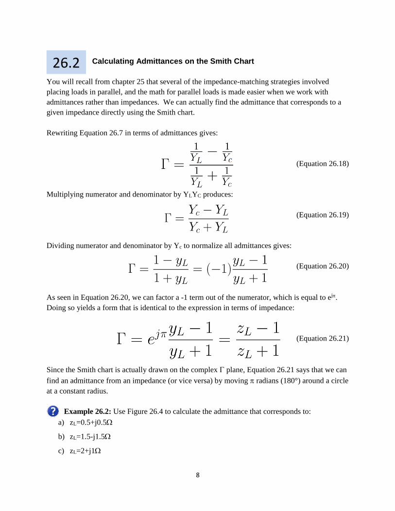
Calculating Admittances on the Smith Chart
You will recall from chapter 25 that several of the impedance-matching strategies involved
placing loads in parallel, and the math for parallel loads is made easier when we work with
admittances rather than impedances. We can actually find the admittance that corresponds to a
given impedance directly using the Smith chart.
Rewriting Equation 26.7 in terms of admittances gives:
(Equation 26.18)
Multiplying numerator and denominator by YLYC produces:
(Equation 26.19)
Dividing numerator and denominator by Yc to normalize all admittances gives:
(Equation 26.20)
As seen in Equation 26.20, we can factor a -1 term out of the numerator, which is equal to ej.
Doing so yields a form that is identical to the expression in terms of impedance:
(Equation 26.21)
Since the Smith chart is actually drawn on the complex plane, Equation 26.21 says that we can
find an admittance from an impedance (or vice versa) by moving radians (180°) around a circle
at a constant radius.
Example 26.2: Use Figure 26.4 to calculate the admittance that corresponds to:
a) zL=0.5+j0.5
b) zL=1.5-j1.5
c) zL=2+j1
26.2

9
Calculating Input Impedance Using a Smith Chart
We can also use a Smith chart to determine the impedance at any point along the line, including
the input impedance at the generator (the opposite end from the load). Recall from chapter 25
that we have the following expression for the impedance at any point z:
(Copy of Equation 25.2)
Since the input impedance is the impedance at z=-L, we can write:
(Equation 26.22)
If we divide both sides of the equation by Zc and then divide the numerator and denominator of
the right side by ejkL, we find:
(Equation 26.23)
We can combine the angle from the load with the phase shift introduced by moving from the
load to the input to obtain:
(Equation 26.24)
Where:
(Equation 26.25)
More generally, if you want to move a distance z’ away from the load, this angle is:
This means that if you know the impedance at any point along the line (such as at the load), you
can simply rotate around the Smith chart an angle of 2kz’ to find it at a different location along
the line. To move toward the generator, you rotate clockwise (a negative angle), and to move
toward the load, you rotate counter-clockwise (a positive angle). It is easier to think of
moving a certain number z’ in wavelengths around the circle, and the 4 term indicates that a
26.3

10
full revolution (2) will be completed when L = /2. This fits perfectly with our earlier
observation that the impedance along the line will repeat once every half wavelength.
Notice that the outer perimeter of the Smith chart is marked off in fractions of a wavelength, with
the number increasing as we move clockwise (toward the generator) on the outer ring and
increasing as we go counterclockwise (toward the generator) on the inner ring. This is illustrated
in Figure 26.5.
Figure 26.5. Moving along the line by rotating around the Smith chart (© 2015 IEEE, used with
permission)
Example 26.3: A line with a characteristic impedance of 50 is terminated in a load
impedance of 75+j50. The line is 5m long, and the wavelength is 1.2m. Use Figure 26.5 to
estimate the input impedance of this line.

11
Designing a Single-Stub Tuner Using a Smith Chart
We can also use the Smith chart to design a single-stub tuner, which was first introduced in
chapter 25. Recall that performing this design consists of determining the distance d1 from the
load where a stub needs to be placed, as well as d2, the length of the stub. We have equations to
perform this calculation, but the Smith chart method is more intuitive and better helps you
understand why the lengths of d1 and d2 must take on certain values.
Before proceeding, let’s consider a very special point and a very special circle on the Smith
chart. The red point in Figure 26.6 corresponds to zL=1+j0, which only occurs when ZL=Zc.
Recall that this is the condition for impedance matching, which means there are no reflections.
The red point in the very center of the Smith chart is always our ultimate destination when
performing impedance matching.
Figure 26.6. Perfect Impedance Matching (Red Dot) and Real Impedance Matching (Green Circle)
(© 2015 IEEE, used with permission)
26.4

12
The green circle corresponds to r=1, which means that the real part of the impedance is matched.
If we can get anywhere onto the green circle, then we will be halfway home, because the real
part of the load impedance will be matched. Once that has happened, we will observe the value
of x at the point where we are, and we will design a stub that has an equal and opposite x,
canceling out the incorrect imaginary part of the load and bringing us to the red dot.
When solving a problem like this, you are actually solving two problems. The first is to
determine d1 by rotating around the Smith chart until you intersect the r=1 circle, and then you
solve a completely different problem by beginning with zL=0 (a short-circuited stub) and
working your way toward the generator until you get to the right value of x to cancel the
imaginary part of the point on the r=1 line to determine d2.
Here is a step-by-step solution method for such a problem:
1. Calculate v, k, and if necessary.
2. Normalize the load impedance.
3. Plot the normalized load impedance
4. Convert the normalized load impedance to an admittance.
5. Rotate around the Smith chart from the load admittance until you hit the r=1 circle.
6. Determine how many wavelengths you rotated and convert this to a length d1.
7. Observe the imaginary admittance x at the point where you intersected the r=1 line.
8. Plot the points where ystub=∞, which corresponds to a short-circuited stub.
9. Rotate clockwise until the imaginary admittance is equal and opposite to that of step 7.
10. Determine how many wavelengths you rotated and convert this to a length d2.
Example 26.4: A line with a characteristic impedance of 100 is terminated in a load
impedance of 70j170. Design a single-stub tuner to match the impedance of this load with
the line. Use the Smith chart of Figure 26.6. The relative dielectric constant of the transmission
line is 4, and the frequency of the transmitter is 100MHz.

13
Summary
The Smith chart is a graphical tool that shows r-circles and x-circles drawn on the complex
plane.
All impedances are normalized by dividing by the characteristic impedance of the line:
Beginning with the equation for the reflection coefficient, we can derive two equations.
These represent the r-circles and x-circles:
You can plot an impedance by looking for the intersection of the appropriate r-circle and x-
circle.
The corresponding admittance can be found by rotating 180°.
The input impedance of a line terminated in a normalized load impedance can be found by
beginning at the point that corresponds to the load impedance and then rotating a distance L
clockwise measured in wavelengths. Rotating clockwise always corresponds to moving
away from the load, while rotating counter-clockwise corresponds to moving toward the
load.
A single-stub tuner is designed by first plotting the (normalized) load impedance, then
converting it to an admittance, then rotating clockwise (away from the load) until you interest
the r=1 circle. Convert the angle rotated to d1. Then begin with ystub=∞ (a short-circuited
stub) and rotate clockwise until you reach an imaginary impedance that is equal and opposite
to the imaginary component of your point on the r=1 circle. Convert the distance rotated to
d2.
26.5