Embed Size (px)
Citation preview

2
•Some history•"Fishers biggest blunder" - the fiducial argument•Confidence distributions and confidence curves•Neyman-Pearson lemma •Confidence and likelihood•Combining information•To bias-correct or not to bias-correct•Box-shaped confidence curves - nested families of confidence bands
•ApplicationsQuantile regression on Norwegian income dataAbundance of bowhead whales from Alaskan photo-ID
data
Outline

3
History
Laplace 1774-1786• Inverse probability: Bayesian
posteriors from flat priors
( ) ( )( )
;;
f xp
f x t dtθ
θ =∫

4
R.A. Fisher (1930) Inverse probability
"to end 150 years of fog and confusion". "I know of only one case in mathematics .. accepted .. by the most eminent men [Laplace and Gauss...] ...to be fundamentally false and devoid of foundation. Yet that is exactly the position in respect to inverse probability ..error on a question of prime theoretical importance...Inverse probability has, I beleive, survived so long in spite of its unsatisfactory basis, because its critics have until recent times put forward nothing to replace it as a rational theory of learning by experience."

5
Pivots•Have the same distributionregardless of the parameter•Are monotoneous (increasing) in the parameter a.s.
( )( )( )
,
, obsfidu
piv X F
F piv X
θ
θ θ
:
:
ExampleThe chi-square pivot for theempirical variance at vdegrees of freedom yieldsthe fiducial cdf:Fiducial density:
( )
( ) ( )
2
2
2
2
2 2'
3 2
1
2
obs
obs obs
s K
sC K
s sc C k
ν
ν
ν
νσ
νσσ
ν νσ σσ σ
⎛ ⎞= − ⎜ ⎟
⎝ ⎠⎛ ⎞
= = ⎜ ⎟⎝ ⎠
:

6
Jerzy Neyman 1930-1941•Confidence intervals and regions•Optimality of tests and confidenceregions under monotoneous likelihoodratio•Confidence intervals are obtainedfrom fiducial distributions:
1
1
1
1
212
12
2
obs
v
obs
v
vs CK
vs CK
αα
αα
−
−
−
−
⎛ ⎞= ⎜ ⎟⎛ ⎞ ⎝ ⎠−⎜ ⎟⎝ ⎠
⎛ ⎞= −⎜ ⎟⎛ ⎞ ⎝ ⎠⎜ ⎟⎝ ⎠

7
Alan Birnbaum 1961: Confidence curves: an omnibus technique for estimation and testing statistical hypotheses.
”incorporatingconfidence intervalsand limits at variouslimits”
For severalparameters ”analogous methods…nested families ofconfidence regions”.
sigma
Con
fiden
ce
0 1 2 3 4 5
0.0
0.2
0.4
0.6
0.8
1.0
Confidence cdf, chi-squar pivot, df=5
sigma
0 1 2 3 4 5
0.0
0.2
0.4
0.6
0.8
1.0
Birnbaum's confidence curve
sigma
degr
ee o
f con
fiden
ce
0 1 2 3 4 5
0.0
0.2
0.4
0.6
0.8
1.0
Confidence curve
sigmaco
nfid
ence
den
sity
0 1 2 3 4 5
0.0
0.4
0.8
1.2
Confidence density

8sigma
degr
ee o
f con
fiden
ce
0 1 2 3 4 5
0.0
0.2
0.4
0.6
0.8
1.0
10 simulated replicates, chi-sqr pivot, df=5

9
The Bayesian counterrevolution• Distributional inference.• Uncertainty presented as posterior distributions.• Rational updating of information.• Integrates judgemental and empirical information. • Computational power and versatility: MCMC.
But• The posterior distribution (and likelihood inference) might be
biased.• Prior distributions are needed, even when no information is
available. Flat prior densities are still “informative”.• The interpretation of the posterior distribution is unclear when the
prior distribution is not a probability distribution.

10
B. Efron1987: Better bootstrap confidence intervals
Efron. 1998. R.A. Fisher in the 21st CenturyFiducial probability = “Fisher's biggest blunder”“I believe that objective Bayes methods will develop for such problems, and that something like fiducial inference will play an important role in this development. Maybe Fisher's biggest blunder will become a big hit in the 21st century!”“applied statistics seems to need an effective compromise betweenBayesian and frequentist ideas, and right now there is no substitute in sight for the Fisherian synthesis.”Fiducial distribution = confidence distribution
( ) ( )ˆ ˆˆ
( ,1)1
h h
N ba
θ γ θ γγ γ
γ
= =
−+
:

11
The fate of the fiducial argument – can Fisher and Neyman agree?
“Both Fisher and Neyman would probably have protested against theuse of confidence distributions” (Efron 1998)
"Fisher was intuitively fully convinced of the importance of "fiducialinference", which he considered the jewel in the crown of the "ideas and nomenclature" for which he was responsible" (Zabel 1992)
"most statisticians, unable to separate the good from the bad in Fisher's arguments, considered the whole fiducial argument Fisher's biggest blunder, or his one great failure, and the whole area fell into disrepute”(Hampel 2002)
The fiducial argument builds a "bridge between aleatory probabilities (the only ones used by Neyman) and epistemic probabilities (the only ones used by Bayesians), by implicitly introducing, as a new type, frequentist epistemic probabilities." (Hampel 2002)

12
Hampel (2002): The fiducial argument builds a "bridge between aleatoryprobabilities (the only ones used by Neyman) and epistemic probabilities (the only ones used by Bayesians), by implicitly introducing, as a new type, frequentist epistemic probabilities.“
•probability is a good term for aleatory probability •confidence for epistemic "probability“ – the currency of digested information•likelihood – the currency of raw information in data, brings probability and confidence together
•Confidence distributions are not sigma-additive! It distributesconfidence over intervals or nested families of regions•Dimensions cannot automatically be reduced by integration.•The confidence curve focus on confidence over regions

13
Neyman-Pearson lemma (Schweder and Hjort 2002)
A confidence distribution based on a sufficient statistic S with monotone likelihood ratio in a scalar parameter is uniformly most powerful: For any value of the parameter, and For any spread functional about itThe spread of the confidencedistribution based on S is stochastically less than that based onanother statistic T.
( ) ( )( ) ( ) ( )
( ) ( )0
0
| | 0 0
S T
ST
t
C C d
C Cθ
γ θ θ θ
γ γ
Γ Γ =
= Γ −
≤
∫Z

14
Confidence and likelihoodDeviance
Null distribution cdf
Confidence from deviance
Profile deviance
Null distribution
Confidence from profiledeviance or other pseudo
likelihood
( ) ( ) ( )( )( )( ) ( )( )( ) ( )( ) ( )( )( )( ) ( )( )( ) ( )( )
,
,
ˆ ( )ˆ, ( )
ˆ; 2 log ; / ;
;
; ;
ˆ; 2 log max , ; / ;
;
; ;
; ;
p
p
p
p
D X L X L X
D X F
N X F D X
D X L X L X
D X F
N X F D X
N X F D X
θ
θ
χ
χψ χ
χ χψ χ
χ ψψ χ ψ
θ θ θ
θ
θ θ
ψ ψ χ θ
ψ
ψ ψ
ψ ψ
= −
=
= −
=
=
:
:

15psi
conf
iden
ce
0 10 20 30 40
0.0
0.2
0.4
0.6
0.8
1.0
SimulatedChi-square 1Fieller
Example: Ratio of two regression parameters. Dotted line is chi-square calibration of the profile deviance. The Fieller method is exact. Only ca 87% finite support!

16
psi
sigm
a 1
0 2 4 6 8 10
0.5
1.0
1.5
2.0
2.5
3.0
0.050.10.20.3 0.4 0.5 0.6 0.7 0.8 0.9 0.95 0.975
psi
Con
fiden
ce
0 2 4 6 8 10
0.0
0.2
0.4
0.6
0.8
1.0
from profile deviancefrom F-pivot
Example: Two normal samples, df’s 9 and 4 1
2
σψσ
=

17
m
conf
iden
ce
0 20 40 60 80
0.0
0.2
0.4
0.6
0.8
1.0
Confidence curve, Negative binomial
X = 20, size = 5
From neg. Binomial devianceFrom Poisson deviance
m
Dev
0 20 40 60 80
05
1015
Deviance functions, negative binomial model
X = 20, size = 5
Neg. binom. devianceCalibrated neg.bin devianceCalibrated Poisson devaincsPoisson deviance
Pseudo deviance calibrated to confidence curve.Confidence curve calibrated to approximatedeviance.
( )( ) ( )( )
( ) ( )( )1
;
; ;
; ;
pseudo
pseudo
appr v
D X F
N X F D X
D X K N X
θ
θ
θ
θ θ
θ θ−
=
=
:

18
Combining information
J independent sources.Confidence curvesDeviance functions
Likelihood synthesisK is the chi-square cdfwith sum df
Confidence synthesisSingh, Xie and Strawderman (2005). H double exponential cdf, G the convolution cdf of Jdouble exponentials. Scalar parameter.
( )( )
j
j
N
D
θ
θ
( ) ( )( ) ( )( )
j
j
D D
N K Dν
θ θ
θ θ ν ν
=
≈ =
∑∑
( ) ( )( )( ) ( )( )
1
1 log 1
j
j j
N G H C
H C N
θ θ
θ θ
−
−
=
= ± −
∑
19
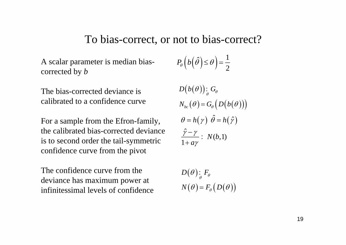
To bias-correct, or not to bias-correct?
( ) ( )ˆ ˆˆ
( ,1)1
h h
N ba
θ γ θ γγ γ
γ
= =
−+
:
A scalar parameter is median bias-corrected by b
The bias-corrected deviance is calibrated to a confidence curve
For a sample from the Efron-family, the calibrated bias-corrected devianceis to second order the tail-symmetricconfidence curve from the pivot
The confidence curve from thedeviance has maximum power at infinitessimal levels of confidence
( )( ) 1ˆ2
P bθ θ θ≤ =
( )( )( ) ( )( )( )bc
D b G
N G D b
θθ
θ
θ
θ θ=
:
( )( ) ( )( )
D F
N F D
θθ
θ
θ
θ θ=
:

20psi
Con
fiden
ce
0 2 4 6 8 10
0.0
0.2
0.4
0.6
0.8
1.0
from bias-corrected deviancefrom F-pivotfrom deviance
Confidence curve for a ratio of two standard deviations
df=9, 4; estimate =2( ) / 0.952b ψ ψ=

21
Application: Four photo surveys of bowhead whales off Barrow, Alaska. Schweder (2003)
1137, 1, 3949, 2, 7520, 3, 6644, 7, 128matures
6211, 0, 999, 0, 6732, 6, 35315, 0, 191immatures
XF85S85F85S 85Survey
# of marked n, recaptured r, and unmarked bowheads u, and # of unique marked X. Spring and Fall 1985-86.

22Abundance
Con
fiden
ce
500 1000 1500 2000 2500
0.0
0.2
0.4
0.6
0.8
1.0
ExactDeviance chi-sq(1)Normal score
Confidence nets for marked mature bowheads
Darroch’s conditionallikelihood for number of unique captures in multiple capture-recapture surveys. Marked mature bowheads only
{ }( ){ }( )
( )1
( )
|
1 |2
( )
( )
obs j
obs j
chi sq
D
P X x n
P X x n
N
K D
θ
θ
θ−
= >
+ =
=

23Marked
Unm
arke
d
500 1000 1500 2000 2500
5000
1000
015
000
2000
0
0.10.20.30.40.50.6
0.70.8
0.9 0.950.99
0.999 0.999
Confidence curve for number of marked and unmarked , 1986. Profiled deviance, simulated null distribution. Schweder (2003).

24
Box-shaped confidence curves for curve-parametersfamilies of simultaneous confidence bands Schweder (2007)
A curve-parameter is of high dimension T.
A box-shaped confidence region is a simultaneousconfidence band.
Beran (1988) adjusts the degree of confidence for a point-wise confidence band to make it a simultaneous confidence band.
When the point-wise confidence curve is based onbootstrapping and Efron’s abc-method, the point-wise confidence curve is adjusted to a box-shapedconfidence curve by the bootstrap distribution ofthe maximum point-wise curve.
( )
( )( ) ( )( ){ }
1
*
*
, ,
max |1 2 |
T
t t
t tt
tbox abc t
H
H K
N K N
θ θ θ
θ
θ
θ θ
=
−
=
L
:
:

25

26
Application: Income and wealth survey, Norway 2002. 22496 Males.95% Quantile regression of capital income on other income (wage), controlled for age. 1000 bootstrap replicates.
other income
95 %
qua
ntile
0 200000 400000 600000 800000
010
0000
2000
0030
0000
4000
00
00.010.50.750.90.950.99

27

28
SummaryConfidence distributions and confidence curves
- provides distributional inference on par with Bayesian posterior distributions, not based on priors
- allows coherent learning
- apply to prediction
- distributes confidence over regions, are not sigma-additive
- might not be proper (the Fieller problem), can be median bias-corrected
- reduce dimension by profiling rather than integration
- keeps aleatory and epistemic probability apart, but provides a bridge between the two: probability vs. confidence
- are transformation invariant
- provides optimal inference in simple models

29
References• Beran, R. 1988. Balanced simultaneous confidence sets. J. Amer. Statis. Assoc. 83: 679-686.• Birnbaum, A. 1961. Confidence curves: an omnibus technique for estimation and testing
statistical hypotheses. J. Amer. Statis. Assoc. 56: 246-249. • Efron, B. 1987. Better bootstrap confidence intervals, (with discussion). J. Amer. Statist.
Assoc. 82, 171–200.• Efron, B. 1998. R.A. Fisher in the 21st century (with discussion). Statistical Science, 13:95-
122.• Fisher, R.A. 1930. Inverse probability. Proc. Cambridge Phil. Society. 26: 528-535.• Hampel, F. 2003. The proper fiducial argument. ftp://ftp.stat.math.ethz.ch/Research-
Reports/114.pdf.• Neyman, J. 1941. Fiducial argument and the theory of confidence intervals. Biometrika 32:
128-150.• Schweder, T. 2003. Abundance estimation from photo-identification data: confidence
distributions and reduced likelihood for bowhead whales off Alaska. Biometrics 59: 976-985.• Schweder, T. 2007. Confidence nets for curves. In Advances in Statistical Modeling and
Inference Essays in Honor of Kjell A. Doksum (ed V. Nair). World Scientific.• Schweder, T. and Hjort, N.L. 2002. Confidence and likelihood. Scandinavian Journal of
Statistics. 29: 309-332.• Singh, K., M. Xie and W.E. Strawderman. 2005. Combining information through confidence
distributions Annals of Statistics 33:159-183.• Zabell S. L. 1992.. R. A. Fisher and the fiducial argument. Statistical Science 7:369--387.