Embed Size (px)
Citation preview

Chapter 22. Using the Solver
This chapter describes the FLUENT solver and how to use it. De-tails about the solver algorithms used by FLUENT are provided in Sec-tions 22.1–22.5. Section 22.6 provides an overview of how to use thesolver, and the remaining sections provide detailed instructions.
• Section 22.1: Overview of Numerical Schemes
• Section 22.2: Discretization
• Section 22.3: Segregated Solver
• Section 22.4: Coupled Solver
• Section 22.5: Multigrid Method
• Section 22.6: Overview of How to Use the Solver
• Section 22.7: Choosing the Discretization Scheme
• Section 22.8: Choosing the Pressure-Velocity Coupling Method
• Section 22.9: Setting Under-Relaxation Factors
• Section 22.10: Changing the Courant Number
• Section 22.11: Turning on FAS Multigrid
• Section 22.12: Setting Solution Limits
• Section 22.13: Initializing the Solution
• Section 22.14: Performing Steady-State Calculations
• Section 22.15: Performing Time-Dependent Calculations
• Section 22.16: Monitoring Solution Convergence
c© Fluent Inc. November 28, 2001 22-1

Using the Solver
• Section 22.17: Animating the Solution
• Section 22.18: Executing Commands During the Calculation
• Section 22.19: Convergence and Stability
22.1 Overview of Numerical Schemes
FLUENT allows you to choose either of two numerical methods:
• segregated solver
• coupled solver
Using either method, FLUENT will solve the governing integral equationsfor the conservation of mass and momentum, and (when appropriate) forenergy and other scalars such as turbulence and chemical species. In bothcases a control-volume-based technique is used that consists of:
• Division of the domain into discrete control volumes using a com-putational grid.
• Integration of the governing equations on the individual controlvolumes to construct algebraic equations for the discrete dependentvariables (“unknowns”) such as velocities, pressure, temperature,and conserved scalars.
• Linearization of the discretized equations and solution of the resul-tant linear equation system to yield updated values of the depen-dent variables.
The two numerical methods employ a similar discretization process (finite-volume), but the approach used to linearize and solve the discretizedequations is different.
The general solution methods are described first in Sections 22.1.1 and22.1.2, followed by a discussion of the linearization methods in Sec-tion 22.1.3.
22-2 c© Fluent Inc. November 28, 2001

22.1 Overview of Numerical Schemes
22.1.1 Segregated Solution Method
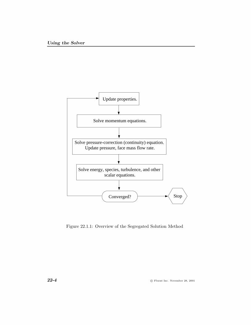
The segregated solver is the solution algorithm previously used by FLU-ENT 4. Using this approach, the governing equations are solved se-quentially (i.e., segregated from one another). Because the governingequations are non-linear (and coupled), several iterations of the solutionloop must be performed before a converged solution is obtained. Eachiteration consists of the steps illustrated in Figure 22.1.1 and outlinedbelow:
1. Fluid properties are updated, based on the current solution. (Ifthe calculation has just begun, the fluid properties will be updatedbased on the initialized solution.)
2. The u, v, and w momentum equations are each solved in turn usingcurrent values for pressure and face mass fluxes, in order to updatethe velocity field.
3. Since the velocities obtained in Step 2 may not satisfy the con-tinuity equation locally, a “Poisson-type” equation for the pres-sure correction is derived from the continuity equation and the lin-earized momentum equations. This pressure correction equationis then solved to obtain the necessary corrections to the pressureand velocity fields and the face mass fluxes such that continuity issatisfied.
4. Where appropriate, equations for scalars such as turbulence, en-ergy, species, and radiation are solved using the previously updatedvalues of the other variables.
5. When interphase coupling is to be included, the source terms inthe appropriate continuous phase equations may be updated witha discrete phase trajectory calculation.
6. A check for convergence of the equation set is made.
These steps are continued until the convergence criteria are met.
c© Fluent Inc. November 28, 2001 22-3
Using the Solver
Update properties.
Solve momentum equations.
Solve pressure-correction (continuity) equation. Update pressure, face mass flow rate.
Solve energy, species, turbulence, and other scalar equations.
Converged? Stop
Figure 22.1.1: Overview of the Segregated Solution Method
22-4 c© Fluent Inc. November 28, 2001

22.1 Overview of Numerical Schemes
22.1.2 Coupled Solution Method
The coupled solver solves the governing equations of continuity, momen-tum, and (where appropriate) energy and species transport simultane-ously (i.e., coupled together). Governing equations for additional scalarswill be solved sequentially (i.e., segregated from one another and fromthe coupled set) using the procedure described for the segregated solverin Section 22.1.1. Because the governing equations are non-linear (andcoupled), several iterations of the solution loop must be performed be-fore a converged solution is obtained. Each iteration consists of the stepsillustrated in Figure 22.1.2 and outlined below:
1. Fluid properties are updated, based on the current solution. (Ifthe calculation has just begun, the fluid properties will be updatedbased on the initialized solution.)
2. The continuity, momentum, and (where appropriate) energy andspecies equations are solved simultaneously.
3. Where appropriate, equations for scalars such as turbulence andradiation are solved using the previously updated values of theother variables.
4. When interphase coupling is to be included, the source terms inthe appropriate continuous phase equations may be updated witha discrete phase trajectory calculation.
5. A check for convergence of the equation set is made.
These steps are continued until the convergence criteria are met.
c© Fluent Inc. November 28, 2001 22-5

Using the Solver
Update properties.
Solve continuity, momentum, energy, and species equations simultaneously.
Solve turbulence and other scalar equations.
Converged? Stop
Figure 22.1.2: Overview of the Coupled Solution Method
22-6 c© Fluent Inc. November 28, 2001

22.1 Overview of Numerical Schemes
22.1.3 Linearization: Implicit vs. Explicit
In both the segregated and coupled solution methods the discrete, non-linear governing equations are linearized to produce a system of equationsfor the dependent variables in every computational cell. The resultantlinear system is then solved to yield an updated flow-field solution.
The manner in which the governing equations are linearized may takean “implicit” or “explicit” form with respect to the dependent variable(or set of variables) of interest. By implicit or explicit we mean thefollowing:
• implicit: For a given variable, the unknown value in each cell iscomputed using a relation that includes both existing and unknownvalues from neighboring cells. Therefore each unknown will appearin more than one equation in the system, and these equations mustbe solved simultaneously to give the unknown quantities.
• explicit: For a given variable, the unknown value in each cell is com-puted using a relation that includes only existing values. Thereforeeach unknown will appear in only one equation in the system andthe equations for the unknown value in each cell can be solved oneat a time to give the unknown quantities.
In the segregated solution method each discrete governing equation islinearized implicitly with respect to that equation’s dependent variable.This will result in a system of linear equations with one equation foreach cell in the domain. Because there is only one equation per cell,this is sometimes called a “scalar” system of equations. A point implicit(Gauss-Seidel) linear equation solver is used in conjunction with an al-gebraic multigrid (AMG) method to solve the resultant scalar systemof equations for the dependent variable in each cell. For example, thex-momentum equation is linearized to produce a system of equations inwhich u velocity is the unknown. Simultaneous solution of this equationsystem (using the scalar AMG solver) yields an updated u-velocity field.
In summary, the segregated approach solves for a single variable field(e.g., p) by considering all cells at the same time. It then solves for the
c© Fluent Inc. November 28, 2001 22-7
Using the Solver
next variable field by again considering all cells at the same time, andso on. There is no explicit option for the segregated solver.
In the coupled solution method you have a choice of using either an im-plicit or explicit linearization of the governing equations. This choiceapplies only to the coupled set of governing equations. Governing equa-tions for additional scalars that are solved segregated from the coupledset, such as for turbulence, radiation, etc., are linearized and solved im-plicitly using the same procedures as in the segregated solution method.Regardless of whether you choose the implicit or explicit scheme, thesolution procedure shown in Figure 22.1.2 is followed.
If you choose the implicit option of the coupled solver, each equationin the coupled set of governing equations is linearized implicitly withrespect to all dependent variables in the set. This will result in a systemof linear equations with N equations for each cell in the domain, whereN is the number of coupled equations in the set. Because there are Nequations per cell, this is sometimes called a “block” system of equations.A point implicit (block Gauss-Seidel) linear equation solver is used inconjunction with an algebraic multigrid (AMG) method to solve theresultant block system of equations for all N dependent variables ineach cell. For example, linearization of the coupled continuity, x-, y-, z-momentum, and energy equation set will produce a system of equationsin which p, u, v, w, and T are the unknowns. Simultaneous solutionof this equation system (using the block AMG solver) yields at onceupdated pressure, u-, v-, w-velocity, and temperature fields.
In summary, the coupled implicit approach solves for all variables (p, u,v, w, T ) in all cells at the same time.
If you choose the explicit option of the coupled solver, each equationin the coupled set of governing equations is linearized explicitly. As inthe implicit option, this too will result in a system of equations withN equations for each cell in the domain. And likewise, all dependentvariables in the set will be updated at once. However, this system ofequations is explicit in the unknown dependent variables. For example,the x-momentum equation is written such that the updated x velocityis a function of existing values of the field variables. Because of this,a linear equation solver is not needed. Instead, the solution is updated
22-8 c© Fluent Inc. November 28, 2001

22.2 Discretization
using a multi-stage (Runge-Kutta) solver. Here you have the additionaloption of employing a full approximation storage (FAS) multigrid schemeto accelerate the multi-stage solver.
In summary, the coupled explicit approach solves for all variables (p, u,v, w, T ) one cell at a time.
Note that the FAS multigrid is an optional component of the explicitapproach, while the AMG is a required element in both the segregatedand coupled implicit approaches.
22.2 Discretization
FLUENT uses a control-volume-based technique to convert the governingequations to algebraic equations that can be solved numerically. Thiscontrol volume technique consists of integrating the governing equationsabout each control volume, yielding discrete equations that conserve eachquantity on a control-volume basis.
Discretization of the governing equations can be illustrated most easilyby considering the steady-state conservation equation for transport ofa scalar quantity φ. This is demonstrated by the following equationwritten in integral form for an arbitrary control volume V as follows:
∮ρφ~v · d ~A =
∮Γφ ∇φ · d ~A+
∫VSφ dV (22.2-1)
whereρ = density~v = velocity vector (= u ı+ v in 2D)~A = surface area vectorΓφ = diffusion coefficient for φ∇φ = gradient of φ (= ∂φ/∂x) ı + (∂φ/∂y) in 2D)Sφ = source of φ per unit volume
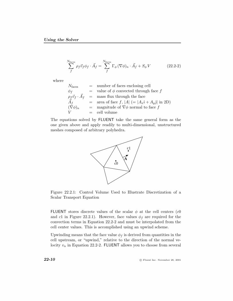
Equation 22.2-1 is applied to each control volume, or cell, in the com-putational domain. The two-dimensional, triangular cell shown in Fig-ure 22.2.1 is an example of such a control volume. Discretization ofEquation 22.2-1 on a given cell yields
c© Fluent Inc. November 28, 2001 22-9
Using the Solver
Nfaces∑f
ρf~vfφf · ~Af =Nfaces∑
f
Γφ (∇φ)n · ~Af + Sφ V (22.2-2)
whereNfaces = number of faces enclosing cellφf = value of φ convected through face fρf~vf · ~Af = mass flux through the face~Af = area of face f , |A| (= |Axı+Ay | in 2D)(∇φ)n = magnitude of ∇φ normal to face fV = cell volume
The equations solved by FLUENT take the same general form as theone given above and apply readily to multi-dimensional, unstructuredmeshes composed of arbitrary polyhedra.
c0
c1
A
Figure 22.2.1: Control Volume Used to Illustrate Discretization of aScalar Transport Equation
FLUENT stores discrete values of the scalar φ at the cell centers (c0and c1 in Figure 22.2.1). However, face values φf are required for theconvection terms in Equation 22.2-2 and must be interpolated from thecell center values. This is accomplished using an upwind scheme.
Upwinding means that the face value φf is derived from quantities in thecell upstream, or “upwind,” relative to the direction of the normal ve-locity vn in Equation 22.2-2. FLUENT allows you to choose from several
22-10 c© Fluent Inc. November 28, 2001

22.2 Discretization
upwind schemes: first-order upwind, second-order upwind, power law,and QUICK. These schemes are described in Sections 22.2.1–22.2.4.
The diffusion terms in Equation 22.2-2 are central-differenced and arealways second-order accurate.
22.2.1 First-Order Upwind Scheme
When first-order accuracy is desired, quantities at cell faces are deter-mined by assuming that the cell-center values of any field variable rep-resent a cell-average value and hold throughout the entire cell; the facequantities are identical to the cell quantities. Thus when first-order up-winding is selected, the face value φf is set equal to the cell-center valueof φ in the upstream cell
22.2.2 Power-Law Scheme
The power-law discretization scheme interpolates the face value of avariable, φ, using the exact solution to a one-dimensional convection-diffusion equation
∂
∂x(ρuφ) =
∂
∂xΓ∂φ
∂x(22.2-3)
where Γ and ρu are constant across the interval ∂x. Equation 22.2-3 canbe integrated to yield the following solution describing how φ varies withx:
φ(x) − φ0
φL − φ0=
exp(Pe xL) − 1
exp(Pe) − 1(22.2-4)
where
φ0 = φ|x=0
φL = φ|x=L
and Pe is the Peclet number:
Pe =ρuL
Γ(22.2-5)
c© Fluent Inc. November 28, 2001 22-11

Using the Solver
The variation of φ(x) between x = 0 and x = L is depicted in Fig-ure 22.2.2 for a range of values of the Peclet number. Figure 22.2.2 showsthat for large Pe, the value of φ at x = L/2 is approximately equal tothe upstream value. This implies that when the flow is dominated byconvection, interpolation can be accomplished by simply letting the facevalue of a variable be set equal to its “upwind” or upstream value. Thisis the standard first-order scheme for FLUENT.
P = 0
P < -1
P = -1
P = 1
P > 1
e
e
e
e
e
0 L
φ
φ
φL
0
X
Figure 22.2.2: Variation of a Variable φ Between x = 0 and x = L(Equation 22.2-3)
If the power-law scheme is selected, FLUENT uses Equation 22.2-4 in anequivalent “power law” format [172], as its interpolation scheme.
As discussed in Section 22.2.1, Figure 22.2.2 shows that for large Pe, thevalue of φ at x = L/2 is approximately equal to the upstream value.When Pe=0 (no flow, or pure diffusion), Figure 22.2.2 shows that φmay be interpolated using a simple linear average between the values atx = 0 and x = L. When the Peclet number has an intermediate value,the interpolated value for φ at x = L/2 must be derived by applying the“power law” equivalent of Equation 22.2-4.
22-12 c© Fluent Inc. November 28, 2001

22.2 Discretization
22.2.3 Second-Order Upwind Scheme
When second-order accuracy is desired, quantities at cell faces are com-puted using a multidimensional linear reconstruction approach [7]. Inthis approach, higher-order accuracy is achieved at cell faces through aTaylor series expansion of the cell-centered solution about the cell cen-troid. Thus when second-order upwinding is selected, the face value φf
is computed using the following expression:
φf = φ+ ∇φ · ∆~s (22.2-6)
where φ and ∇φ are the cell-centered value and its gradient in the up-stream cell, and ∆~s is the displacement vector from the upstream cellcentroid to the face centroid. This formulation requires the determina-tion of the gradient ∇φ in each cell. This gradient is computed usingthe divergence theorem, which in discrete form is written as
∇φ =1V
Nfaces∑f
φf~A (22.2-7)
Here the face values φf are computed by averaging φ from the two cellsadjacent to the face. Finally, the gradient ∇φ is limited so that no newmaxima or minima are introduced.
22.2.4 QUICK Scheme
For quadrilateral and hexahedral meshes, where unique upstream anddownstream faces and cells can be identified, FLUENT also provides theQUICK scheme for computing a higher-order value of the convected vari-able φ at a face. QUICK-type schemes [133] are based on a weightedaverage of second-order-upwind and central interpolations of the vari-able. For the face e in Figure 22.2.3, if the flow is from left to right, sucha value can be written as
c© Fluent Inc. November 28, 2001 22-13

Using the Solver
φe = θ
[Sd
Sc + SdφP +
Sc
Sc + SdφE
]+ (1− θ)
[Su + 2Sc
Su + ScφP − Sc
Su + ScφW
](22.2-8)
W P E
w e
∆xe∆xw
Su Sc Sd
Figure 22.2.3: One-Dimensional Control Volume
θ = 1 in the above equation results in a central second-order interpolationwhile θ = 0 yields a second-order upwind value. The traditional QUICKscheme is obtained by setting θ = 1/8. The implementation in FLUENTuses a variable, solution-dependent value of θ, chosen so as to avoidintroducing new solution extrema.
The QUICK scheme will typically be more accurate on structured gridsaligned with the flow direction. Note that FLUENT allows the use ofthe QUICK scheme for unstructured or hybrid grids as well; in suchcases the usual second-order upwind discretization scheme (describedin Section 22.2.3) will be used at the faces of non-hexahedral (or non-quadrilateral, in 2D) cells. The second-order upwind scheme will also beused at partition boundaries when the parallel solver is used.
22.2.5 Central-Differencing Scheme
A second-order-accurate central-differencing discretization scheme is avail-able for the momentum equations when you are using the LES turbulencemodel. This scheme provides improved accuracy for LES calculations.
The central-differencing scheme calculates the face value for a variable(φf ) as follows:
22-14 c© Fluent Inc. November 28, 2001

22.2 Discretization
φf,CD =12
(φ0 + φ1) +12
(∇φr,0 · ~r0 + ∇φr,1 · ~r1) (22.2-9)
where the indices 0 and 1 refer to the cells that share face f , ∇φr,0 and∇φr,1 are the reconstructed gradients at cells 0 and 1, respectively, and~r is the vector directed from the cell centroid toward the face centroid.
It is well known that central-differencing schemes can produce unboundedsolutions and non-physical wiggles, which can lead to stability prob-lems for the numerical procedure. These stability problems can often beavoided if a deferred approach is used for the central-differencing scheme.In this approach, the face value is calculated as follows:
φf = φf,UP︸ ︷︷ ︸implicit part
+ (φf,CD − φf,UP)︸ ︷︷ ︸explicit part
(22.2-10)
where UP stands for upwind. As indicated, the upwind part is treatedimplicitly while the difference between the central-difference and upwindvalues is treated explicitly. Provided that the numerical solution con-verges, this approach leads to pure second-order differencing.
22.2.6 Linearized Form of the Discrete Equation
The discretized scalar transport equation (Equation 22.2-2) contains theunknown scalar variable φ at the cell center as well as the unknownvalues in surrounding neighbor cells. This equation will, in general, benon-linear with respect to these variables. A linearized form of Equa-tion 22.2-2 can be written as
aP φ =∑nb
anbφnb + b (22.2-11)
where the subscript nb refers to neighbor cells, and aP and anb are thelinearized coefficients for φ and φnb.
c© Fluent Inc. November 28, 2001 22-15

Using the Solver
The number of neighbors for each cell depends on the grid topology, butwill typically equal the number of faces enclosing the cell (boundary cellsbeing the exception).
Similar equations can be written for each cell in the grid. This resultsin a set of algebraic equations with a sparse coefficient matrix. Forscalar equations, FLUENT solves this linear system using a point implicit(Gauss-Seidel) linear equation solver in conjunction with an algebraicmultigrid (AMG) method which is described in Section 22.5.3.
22.2.7 Under-Relaxation
Because of the nonlinearity of the equation set being solved by FLUENT,it is necessary to control the change of φ. This is typically achieved byunder-relaxation, which reduces the change of φ produced during eachiteration. In a simple form, the new value of the variable φ within a celldepends upon the old value, φold, the computed change in φ, ∆φ, andthe under-relaxation factor, α, as follows:
φ = φold + α∆φ (22.2-12)
22.2.8 Temporal Discretization
For transient simulations, the governing equations must be discretized inboth space and time. The spatial discretization for the time-dependentequations is identical to the steady-state case. Temporal discretizationinvolves the integration of every term in the differential equations over atime step ∆t. The integration of the transient terms is straightforward,as shown below.
A generic expression for the time evolution of a variable φ is given by
∂φ
∂t= F (φ) (22.2-13)
where the function F incorporates any spatial discretization. If the timederivative is discretized using backward differences, the first-order accu-rate temporal discretization is given by
22-16 c© Fluent Inc. November 28, 2001

22.2 Discretization
φn+1 − φn
∆t= F (φ) (22.2-14)
and the second-order discretization is given by
3φn+1 − 4φn + φn−1
2∆t= F (φ) (22.2-15)
where
φ = a scalar quantityn+ 1 = value at the next time level, t+ ∆tn = value at the current time level, tn− 1 = value at the previous time level, t− ∆t
Once the time derivative has been discretized, a choice remains for eval-uating F (φ): in particular, which time level values of φ should be usedin evaluating F?
Implicit Time Integration
One method is to evaluate F (φ) at the future time level:
φn+1 − φn
∆t= F (φn+1) (22.2-16)
This is referred to as “implicit” integration since φn+1 in a given cell isrelated to φn+1 in neighboring cells through F (φn+1):
φn+1 = φn + ∆tF (φn+1) (22.2-17)
This implicit equation can be solved iteratively by initializing φi to φn
and iterating the equation
φi = φn + ∆tF (φi) (22.2-18)
for the first-order implicit formulation, or
c© Fluent Inc. November 28, 2001 22-17

Using the Solver
φi = 4/3φn − 1/3φn−1 + 2/3∆tF (φi) (22.2-19)
for the second-order implicit formulation, until φi stops changing (i.e.,converges). At that point, φn+1 is set to φi.
The advantage of the fully implicit scheme is that it is unconditionallystable with respect to time step size.
Explicit Time Integration
A second method is available when the coupled explicit solver is used.This method evaluates F (φ) at the current time level:
φn+1 − φn
∆t= F (φn) (22.2-20)
and is referred to as “explicit” integration since φn+1 can be expressedexplicitly in terms of the existing solution values, φn:
φn+1 = φn + ∆tF (φn) (22.2-21)
(This method is also referred to as “global time stepping”.)
Here, the time step ∆t is restricted to the stability limit of the underlyingsolver (i.e., a time step corresponding to a Courant number of approxi-mately 1). In order to be time-accurate, all cells in the domain must usethe same time step. For stability, this time step must be the minimumof all the local time steps in the domain.
The use of explicit time stepping is fairly restrictive. It is used primar-ily to capture the transient behavior of moving waves, such as shocks,because it is more accurate and less expensive than the implicit timestepping methods in such cases. You cannot use explicit time steppingin the following cases:
• Calculations with the segregated or coupled implicit solver. Theexplicit time stepping formulation is available only with the coupledexplicit solver.
22-18 c© Fluent Inc. November 28, 2001
22.2 Discretization
• Incompressible flow. Explicit time stepping cannot be used to com-pute time-accurate incompressible flows (i.e., gas laws other thanideal gas). Incompressible solutions must be iterated to conver-gence within each time step.
• Convergence acceleration. FAS multigrid and residual smoothingcannot be used with explicit time stepping because they destroythe time accuracy of the underlying solver.
c© Fluent Inc. November 28, 2001 22-19
Using the Solver
22.3 The Segregated Solver
In this section, special practices related to the discretization of the mo-mentum and continuity equations and their solution by means of the seg-regated solver are addressed. These practices are most easily describedby considering the steady-state continuity and momentum equations inintegral form:
∮ρ~v · d ~A = 0 (22.3-1)
∮ρ~v ~v · d ~A = −
∮pI · d ~A+
∮τ · d ~A+
∫V
~F dV (22.3-2)
where I is the identity matrix, τ is the stress tensor, and ~F is the forcevector.
22.3.1 Discretization of the Momentum Equation
The discretization scheme described in Section 22.2 for a scalar trans-port equation is also used to discretize the momentum equations. Forexample, the x-momentum equation can be obtained by setting φ = u:
aP u =∑nb
anb unb +∑
pfA · ı+ S (22.3-3)
If the pressure field and face mass fluxes were known, Equation 22.3-3could be solved in the manner outlined in Section 22.2, and a velocityfield obtained. However, the pressure field and face mass fluxes are notknown a priori and must be obtained as a part of the solution. Thereare important issues with respect to the storage of pressure and thediscretization of the pressure gradient term; these are addressed next.
FLUENT uses a co-located scheme, whereby pressure and velocity areboth stored at cell centers. However, Equation 22.3-3 requires the valueof the pressure at the face between cells c0 and c1, shown in Figure 22.2.1.Therefore, an interpolation scheme is required to compute the face valuesof pressure from the cell values.
22-20 c© Fluent Inc. November 28, 2001

22.3 The Segregated Solver
Pressure Interpolation Schemes
The default scheme in FLUENT interpolates the pressure values at thefaces using momentum equation coefficients [192]. This procedure workswell as long as the pressure variation between cell centers is smooth.When there are jumps or large gradients in the momentum source termsbetween control volumes, the pressure profile has a high gradient at thecell face, and cannot be interpolated using this scheme. If this scheme isused, the discrepancy shows up in overshoots/undershoots of cell veloc-ity.
Flows for which the standard pressure interpolation scheme will havetrouble include flows with large body forces, such as in strongly swirlingflows, in high-Rayleigh-number natural convection and the like. In suchcases, it is necessary to pack the mesh in regions of high gradient toresolve the pressure variation adequately.
Another source of error is that FLUENT assumes that the normal pressuregradient at the wall is zero. This is valid for boundary layers, but not inthe presence of body forces or curvature. Again, the failure to correctlyaccount for the wall pressure gradient is manifested in velocity vectorspointing in/out of walls.
Several alternate methods are available for cases in which the standardpressure interpolation scheme is not valid:
• The linear scheme computes the face pressure as the average of thepressure values in the adjacent cells.
• The second-order scheme reconstructs the face pressure in the man-ner used for second-order accurate convection terms (see Section22.2.3). This scheme may provide some improvement over the stan-dard and linear schemes, but it may have some trouble if it is usedat the start of a calculation and/or with a bad mesh. The second-order scheme is not applicable for flows with discontinuous pressuregradients imposed by the presence of a porous medium in the do-main or the use of the VOF or mixture model for multiphase flow.
• The body-force-weighted scheme computes the face pressure by as-suming that the normal gradient of the difference between pressure
c© Fluent Inc. November 28, 2001 22-21
Using the Solver
and body forces is constant. This works well if the body forces areknown a priori in the momentum equations (e.g., buoyancy andaxisymmetric swirl calculations).
• The PRESTO! (PREssure STaggering Option) scheme uses thediscrete continuity balance for a “staggered” control volume aboutthe face to compute the “staggered” (i.e., face) pressure. This pro-cedure is similar in spirit to the staggered-grid schemes used withstructured meshes [172]. Note that for triangular and tetrahedralmeshes, comparable accuracy is obtained using a similar algorithm.
See Section 22.7.3 for recommendations on when to use these alternateschemes.
22.3.2 Discretization of the Continuity Equation
Equation 22.3-1 may be integrated over the control volume in Figure 22.2.1to yield the following discrete equation
Nfaces∑f
JfAf = 0 (22.3-4)
where Jf is the mass flux through face f , ρvn.
As described in Section 22.1, the momentum and continuity equations aresolved sequentially. In this sequential procedure, the continuity equationis used as an equation for pressure. However, pressure does not appearexplicitly in Equation 22.3-4 for incompressible flows, since density isnot directly related to pressure. The SIMPLE (Semi-Implicit Methodfor Pressure-Linked Equations) family of algorithms [172] is used forintroducing pressure into the continuity equation. This procedure isoutlined in Section 22.3.3.
In order to proceed further, it is necessary to relate the face values ofvelocity, ~vn, to the stored values of velocity at the cell centers. Linearinterpolation of cell-centered velocities to the face results in unphysicalchecker-boarding of pressure. FLUENT uses a procedure similar to thatoutlined by Rhie and Chow [192] to prevent checkerboarding. The face
22-22 c© Fluent Inc. November 28, 2001

22.3 The Segregated Solver
value of velocity is not averaged linearly; instead, momentum-weightedaveraging, using weighting factors based on the aP coefficient from equa-tion 22.3-3, is performed. Using this procedure, the face flux, Jf , maybe written as
Jf = Jf + df (pc0 − pc1) (22.3-5)
where pc0 and pc1 are the pressures within the two cells on either sideof the face, and Jf contains the influence of velocities in these cells (seeFigure 22.2.1). The term df is a function of aP , the average of themomentum equation aP coefficients for the cells on either side of face f .
Density Interpolation Schemes
For compressible flow calculations (i.e., calculations that use the idealgas law for density), FLUENT applies upwind interpolation of density atcell faces. (For incompressible flows, FLUENT uses arithmetic averag-ing.) Three interpolation schemes are available for the density upwind-ing at cell faces: first-order upwind (default), second-order-upwind, andQUICK.
The first-order upwind scheme (based on [109]) sets the density at thecell face to be the upstream cell-center value. This scheme providesstability for the discretization of the pressure-correction equation, andgives good results for most classes of flows. The first-order scheme is thedefault scheme for compressible flows.
The second-order upwind scheme provides stability for supersonic flowsand captures shocks better than the first-order upwind scheme. TheQUICK scheme for density is similar to the QUICK scheme used forother variables. See Section 22.2.4 for details.
The second-order upwind and QUICK schemes for density are not avail-!able for compressible multiphase calculations; the first-order upwindscheme is used for the compressible phase, and arithmetic averaging isused for the incompressible phases.
See Section 22.7.4 for recommendations on choosing an appropriate den-sity interpolation scheme for your compressible flow.
c© Fluent Inc. November 28, 2001 22-23

Using the Solver
22.3.3 Pressure-Velocity Coupling
Pressure-velocity coupling is achieved by using Equation 22.3-5 to derivean equation for pressure from the discrete continuity equation (Equa-tion 22.3-4) FLUENT provides the option to choose among three pressure-velocity coupling algorithms: SIMPLE, SIMPLEC, and PISO. See Sec-tion 22.8 for instructions on how to select these algorithms.
SIMPLE
The SIMPLE algorithm uses a relationship between velocity and pressurecorrections to enforce mass conservation and to obtain the pressure field.
If the momentum equation is solved with a guessed pressure field p∗, theresulting face flux, J∗
f , computed from Equation 22.3-5
J∗f = J∗
f + df (p∗c0 − p∗c1) (22.3-6)
does not satisfy the continuity equation. Consequently, a correction J ′f
is added to the face flux J∗f so that the corrected face flux, Jf
Jf = J∗f + J ′
f (22.3-7)
satisfies the continuity equation. The SIMPLE algorithm postulates thatJ ′
f be written as
J ′f = df (p′c0 − p′c1) (22.3-8)
where p′ is the cell pressure correction.
The SIMPLE algorithm substitutes the flux correction equations (Equa-tions 22.3-7 and 22.3-8) into the discrete continuity equation (Equa-tion 22.3-4) to obtain a discrete equation for the pressure correction p′
in the cell:
aP p′ =
∑nb
anb p′nb + b (22.3-9)
22-24 c© Fluent Inc. November 28, 2001

22.3 The Segregated Solver
where the source term b is the net flow rate into the cell:
b =Nfaces∑
f
J∗fAf (22.3-10)
The pressure-correction equation (Equation 22.3-9) may be solved usingthe algebraic multigrid (AMG) method described in Section 22.5.3. Oncea solution is obtained, the cell pressure and the face flux are correctedusing
p = p∗ + αp p′ (22.3-11)
Jf = J∗f + df (p′c0 − p′c1) (22.3-12)
Here αp is the under-relaxation factor for pressure (see Section 22.2.7for information about under-relaxation). The corrected face flux, Jf ,satisfies the discrete continuity equation identically during each iteration.
SIMPLEC
A number of variants of the basic SIMPLE algorithm are available inthe literature. In addition to SIMPLE, FLUENT offers the SIMPLEC(SIMPLE-Consistent) algorithm [243]. SIMPLE is the default, but manyproblems will benefit from the use of SIMPLEC, as described in Sec-tion 22.8.1.
The SIMPLEC procedure is similar to the SIMPLE procedure outlinedabove. The only difference lies in the expression used for the face fluxcorrection, J ′
f . As in SIMPLE, the correction equation may be writtenas
Jf = J∗f + df (p′c0 − p′c1) (22.3-13)
However, the coefficient df is redefined as a function of (aP −∑nb anb)The use of this modified correction equation has been shown to accelerate
c© Fluent Inc. November 28, 2001 22-25
Using the Solver
convergence in problems where pressure-velocity coupling is the maindeterrent to obtaining a solution.
PISO
The Pressure-Implicit with Splitting of Operators (PISO) pressure-veloc-ity coupling scheme, part of the SIMPLE family of algorithms, is basedon the higher degree of the approximate relation between the correctionsfor pressure and velocity. One of the limitations of the SIMPLE and SIM-PLEC algorithms is that new velocities and corresponding fluxes do notsatisfy the momentum balance after the pressure-correction equation issolved. As a result, the calculation must be repeated until the balanceis satisfied. To improve the efficiency of this calculation, the PISO al-gorithm performs two additional corrections: neighbor correction andskewness correction.
Neighbor Correction
The main idea of the PISO algorithm is to move the repeated calcu-lations required by SIMPLE and SIMPLEC inside the solution stageof the pressure-correction equation [97]. After one or more additionalPISO loops, the corrected velocities satisfy the continuity and momen-tum equations more closely. This iterative process is called a momentumcorrection or “neighbor correction”. The PISO algorithm takes a littlemore CPU time per solver iteration, but it can dramatically decreasethe number of iterations required for convergence, especially for tran-sient problems.
Skewness Correction
For meshes with some degree of skewness, the approximate relationshipbetween the correction of mass flux at the cell face and the differenceof the pressure corrections at the adjacent cells is very rough. Since thecomponents of the pressure-correction gradient along the cell faces arenot known in advance, an iterative process similar to the PISO neighborcorrection described above is desirable [64]. After the initial solutionof the pressure-correction equation, the pressure-correction gradient isrecalculated and used to update the mass flux corrections. This process,
22-26 c© Fluent Inc. November 28, 2001

22.3 The Segregated Solver
which is referred to as “skewness correction”, significantly reduces con-vergence difficulties associated with highly distorted meshes. The PISOskewness correction allows FLUENT to obtain a solution on a highlyskewed mesh in approximately the same number of iterations as requiredfor a more orthogonal mesh.
Special Treatment for Strong Body Forces in Multiphase Flows
When large body forces (e.g., gravity or surface tension forces) existin multiphase flows, the body force and pressure gradient terms in themomentum equation are almost in equilibrium, with the contributions ofconvective and viscous terms small in comparison. Segregated algorithmsconverge poorly unless partial equilibrium of pressure gradient and bodyforces is taken into account. FLUENT provides an optional “implicit bodyforce” treatment that can account for this effect, making the solutionmore robust.
The basic procedure involves augmenting the correction equation forthe face flow rate, Equation 22.3-12, with an additional term involvingcorrections to the body force. This results in extra body force correctionterms in Equation 22.3-10, and allows the flow to achieve a realisticpressure field very early in the iterative process.
This option is available only for multiphase calculations, but it is turnedoff by default. Section 20.6.11 includes instructions for turning on theimplicit body force treatment.
In addition, FLUENT allows you to control the change in the body forcesthrough the use of an under-relaxation factor for body forces.
22.3.4 Steady-State and Time-Dependent Calculations
The governing equations for the segregated solver do not contain anytime-dependent terms if you are performing a steady-state calculation.
For time-accurate calculations, an implicit time stepping scheme is used.See Section 22.2.8 for details.
c© Fluent Inc. November 28, 2001 22-27

Using the Solver
22.4 The Coupled Solver
The coupled solver in FLUENT solves the governing equations of conti-nuity, momentum, and (where appropriate) energy and species transportsimultaneously as a set, or vector, of equations. Governing equations foradditional scalars will be solved sequentially (i.e., segregated from oneanother and from the coupled set).
22.4.1 Governing Equations in Vector Form
The system of governing equations for a single-component fluid, writtento describe the mean flow properties, is cast in integral, Cartesian formfor an arbitrary control volume V with differential surface area dA asfollows:
∂
∂t
∫V
W dV +∮
[F − G] · dA =∫
VH dV (22.4-1)
where the vectors W ,F , and G are defined as
W =
ρρuρvρwρE
, F =
ρvρvu + pıρvv + p
ρvw + pkρvE + pv
, G =
0τxi
τ yi
τ zi
τ ijvj + q
and the vector H contains source terms such as body forces and energysources.
Here ρ, v, E, and p are the density, velocity, total energy per unit mass,and pressure of the fluid, respectively. τ is the viscous stress tensor, andq is the heat flux.
Total energy E is related to the total enthalpy H by
E = H − p/ρ (22.4-2)
where
22-28 c© Fluent Inc. November 28, 2001

22.4 The Coupled Solver
H = h+ |v|2/2 (22.4-3)
The Navier-Stokes equations as expressed in Equation 22.4-1 become(numerically) very stiff at low Mach number due to the disparity betweenthe fluid velocity v and the acoustic speed c (speed of sound). This isalso true for incompressible flows, regardless of the fluid velocity, becauseacoustic waves travel infinitely fast in an incompressible fluid (speedof sound is infinite). The numerical stiffness of the equations underthese conditions results in poor convergence rates. This difficulty isovercome in FLUENT’s coupled solver by employing a technique called(time-derivative) preconditioning [261].
22.4.2 Preconditioning
Time-derivative preconditioning modifies the time-derivative term in Equa-tion 22.4-1 by pre-multiplying it with a preconditioning matrix. This hasthe effect of re-scaling the acoustic speed (eigenvalue) of the system ofequations being solved in order to alleviate the numerical stiffness en-countered in low Mach number and incompressible flow.
Derivation of the preconditioning matrix begins by transforming the de-pendent variable in Equation 22.4-1 from conserved quantities W toprimitive variables Q using the chain-rule as follows:
∂W
∂Q
∂
∂t
∫V
Q dV +∮
[F − G] · dA =∫
VH dV (22.4-4)
where Q is the vector {p, u, v, w, T}T and the Jacobian ∂W /∂Q is givenby
∂W
∂Q=
ρp 0 0 0 ρT
ρpu ρ 0 0 ρTuρpv 0 ρ 0 ρT vρpw 0 0 ρ ρTwρpH − δ ρu ρv ρw ρTH + ρCp
(22.4-5)
c© Fluent Inc. November 28, 2001 22-29

Using the Solver
whereρp =
∂ρ
∂p
∣∣∣∣T
, ρT =∂ρ
∂T
∣∣∣∣p
and δ = 1 for an ideal gas and δ = 0 for an incompressible fluid.
The choice of primitive variables Q as dependent variables is desirablefor several reasons. First, it is a natural choice when solving incom-pressible flows. Second, when we use second-order accuracy we need toreconstruct Q rather than W in order to obtain more accurate velocityand temperature gradients in viscous fluxes, and pressure gradients ininviscid fluxes. And finally, the choice of pressure as a dependent vari-able allows the propagation of acoustic waves in the system to be singledout [245].
We precondition the system by replacing the Jacobian matrix ∂W /∂Q(Equation 22.4-5) with the preconditioning matrix Γ so that the precon-ditioned system in conservation form becomes
Γ∂
∂t
∫V
Q dV +∮
[F − G] · dA =∫
VH dV (22.4-6)
where
Γ =
Θ 0 0 0 ρT
Θu ρ 0 0 ρTuΘv 0 ρ 0 ρTuΘw 0 0 ρ ρTuΘH − δ ρu ρv ρw ρTH + ρCp
(22.4-7)
The parameter Θ is given by
Θ =
(1U2
r
− ρT
ρCp
)(22.4-8)
The reference velocity Ur appearing in Equation 22.4-8 is chosen locallysuch that the eigenvalues of the system remain well conditioned withrespect to the convective and diffusive time scales [261].
22-30 c© Fluent Inc. November 28, 2001
22.4 The Coupled Solver
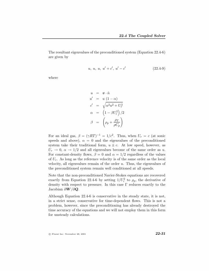
The resultant eigenvalues of the preconditioned system (Equation 22.4-6)are given by
u, u, u, u′ + c′, u′ − c′ (22.4-9)
where
u = v · nu′ = u (1 − α)
c′ =√α2u2 + U2
r
α =(1 − βU2
r
)/2
β =
(ρp +
ρT
ρCp
)
For an ideal gas, β = (γRT )−1 = 1/c2. Thus, when Ur = c (at sonicspeeds and above), α = 0 and the eigenvalues of the preconditionedsystem take their traditional form, u ± c. At low speed, however, asUr → 0, α → 1/2 and all eigenvalues become of the same order as u.For constant-density flows, β = 0 and α = 1/2 regardless of the valuesof Ur. As long as the reference velocity is of the same order as the localvelocity, all eigenvalues remain of the order u. Thus, the eigenvalues ofthe preconditioned system remain well conditioned at all speeds.
Note that the non-preconditioned Navier-Stokes equations are recoveredexactly from Equation 22.4-6 by setting 1/U2
r to ρp, the derivative ofdensity with respect to pressure. In this case Γ reduces exactly to theJacobian ∂W /∂Q.
Although Equation 22.4-6 is conservative in the steady state, it is not,in a strict sense, conservative for time-dependent flows. This is not aproblem, however, since the preconditioning has already destroyed thetime accuracy of the equations and we will not employ them in this formfor unsteady calculations.
c© Fluent Inc. November 28, 2001 22-31
Using the Solver
Flux-Difference Splitting
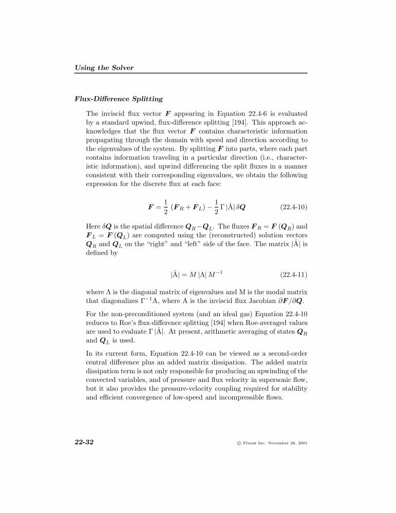
The inviscid flux vector F appearing in Equation 22.4-6 is evaluatedby a standard upwind, flux-difference splitting [194]. This approach ac-knowledges that the flux vector F contains characteristic informationpropagating through the domain with speed and direction according tothe eigenvalues of the system. By splitting F into parts, where each partcontains information traveling in a particular direction (i.e., character-istic information), and upwind differencing the split fluxes in a mannerconsistent with their corresponding eigenvalues, we obtain the followingexpression for the discrete flux at each face:
F =12
(F R + F L) − 12
Γ |A| δQ (22.4-10)
Here δQ is the spatial difference QR−QL. The fluxes F R = F (QR) andF L = F (QL) are computed using the (reconstructed) solution vectorsQR and QL on the “right” and “left” side of the face. The matrix |A| isdefined by
|A| = M |Λ|M−1 (22.4-11)
where Λ is the diagonal matrix of eigenvalues and M is the modal matrixthat diagonalizes Γ−1A, where A is the inviscid flux Jacobian ∂F /∂Q.
For the non-preconditioned system (and an ideal gas) Equation 22.4-10reduces to Roe’s flux-difference splitting [194] when Roe-averaged valuesare used to evaluate Γ |A|. At present, arithmetic averaging of states QR
and QL is used.
In its current form, Equation 22.4-10 can be viewed as a second-ordercentral difference plus an added matrix dissipation. The added matrixdissipation term is not only responsible for producing an upwinding of theconvected variables, and of pressure and flux velocity in supersonic flow,but it also provides the pressure-velocity coupling required for stabilityand efficient convergence of low-speed and incompressible flows.
22-32 c© Fluent Inc. November 28, 2001

22.4 The Coupled Solver
22.4.3 Time Marching for Steady-State Flows
The coupled set of governing equations (Equation 22.4-6) in FLUENTis discretized in time for both steady and unsteady calculations. In thesteady case, it is assumed that time marching proceeds until a steady-state solution is reached. Temporal discretization of the coupled equa-tions is accomplished by either an implicit or an explicit time-marchingscheme. These two algorithms are described below.
Explicit Scheme
In the explicit scheme a multi-stage, time-stepping algorithm [101] isused to discretize the time derivative in Equation 22.4-6. The solutionis advanced from iteration n to iteration n+ 1 with an m-stage Runge-Kutta scheme, given by
Q0 = Qn
∆Qi = −αi∆tΓ−1Ri−1
Qn+1 = Qm
where ∆Qi ≡ Qi − Qn and i = 1, 2, . . . ,m is the stage counter forthe m-stage scheme. αi is the multi-stage coefficient for the ith stage.The residual Ri is computed from the intermediate solution Qi and, forEquation 22.4-6, is given by
Ri =Nfaces∑ (
F (Qi) − G(Qi))· A − VH (22.4-12)
The time step ∆t is computed from the CFL (Courant-Friedrichs-Lewy)condition
∆t =CFL∆xλmax
(22.4-13)
where λmax is the maximum of the local eigenvalues defined by Equa-tion 22.4-9.
c© Fluent Inc. November 28, 2001 22-33

Using the Solver
The convergence rate of the explicit scheme can be accelerated throughuse of the full-approximation storage (FAS) multigrid method describedin Section 22.5.4.
Implicit Residual Smoothing
The maximum time step can be further increased by increasing the sup-port of the scheme through implicit averaging of the residuals with theirneighbors. The residuals are filtered through a Laplacian smoothingoperator:
Ri = Ri + ε∑
(Rj − Ri) (22.4-14)
This equation can be solved with the following Jacobi iteration:
Rmi =
Ri + ε∑Rm−1
j
1 + ε∑
1(22.4-15)
Two Jacobi iterations are usually sufficient to allow doubling the timestep with a value of ε = 0.5.
Implicit Scheme
In the implicit scheme, an Euler implicit discretization in time of thegoverning equations (Equation 22.4-6) is combined with a Newton-typelinearization of the fluxes to produce the following linearized system indelta form [259]:
D +
Nfaces∑j
Sj,k
∆Qn+1 = −Rn (22.4-16)
The center and off-diagonal coefficient matrices, D and Sj,k are given by
D =V
∆tΓ +
Nfaces∑j
Sj,i (22.4-17)
22-34 c© Fluent Inc. November 28, 2001

22.4 The Coupled Solver
Sj,k =(∂F j
∂Qk
− ∂Gj
∂Qk
)(22.4-18)
and the residual vector Rn and time step ∆t are defined as in Equa-tion 22.4-12 and Equation 22.4-13, respectively.
Equation 22.4-16 is solved using a point Gauss-Seidel scheme in con-junction with an algebraic multigrid (AMG) method (see Section 22.5.3)adapted for coupled sets of equations.
22.4.4 Temporal Discretization for Unsteady Flows
For time-accurate calculations, explicit and implicit time-steppingschemes are available. (The implicit approach is also referred to as “dualtime stepping”.)
Explicit Time Stepping
In the explicit time stepping approach, the explicit scheme describedabove is employed, using the same time step in each cell of the domain,and with preconditioning disabled.
Dual Time Stepping
To provide for efficient, time-accurate solution of the preconditionedequations, we employ a dual time-stepping, multi-stage scheme. Herewe introduce a preconditioned pseudo-time-derivative term into Equa-tion 22.4-1 as follows:
∂
∂t
∫V
W dV + Γ∂
∂τ
∫V
Q dV +∮
[F − G] · dA =∫
VH dV (22.4-19)
where t denotes physical-time and τ is a pseudo-time used in the time-marching procedure. Note that as τ → ∞, the second term on the LHSof Equation 22.4-19 vanishes and Equation 22.4-1 is recovered.
The time-dependent term in Equation 22.4-19 is discretized in an implicitfashion by means of either a first- or second-order accurate, backwarddifference in time. This is written in semi-discrete form as follows:
c© Fluent Inc. November 28, 2001 22-35

Using the Solver
[Γ
∆τ+ε0∆t
∂W
∂Q
]∆Qk+1 +
1V
∮[F − G] · dA
= H +1
∆t
(ε0W
k − ε1Wn + ε2W
n−1)
where {ε0 = ε1 = 1/2, ε2 = 0} gives first-order time accuracy, and {ε0 =3/2, ε1 = 2, ε2 = 1/2} gives second-order. k is the inner iteration counterand n represents any given physical-time level.
The pseudo-time-derivative is driven to zero at each physical time levelby a series of inner iterations using either the implicit or explicit time-marching algorithm. Throughout the (inner) iterations in pseudo-time,W n and W n−1 are held constant and W k is computed from Qk. Asτ → ∞, the solution at the next physical time level W n+1 is given byW (Qk).
Note that the physical time step ∆t is limited only by the level of desiredtemporal accuracy. The pseudo-time-step ∆τ is determined by the CFLcondition of the (implicit or explicit) time-marching scheme.
22.5 Multigrid Method
The FLUENT solver contains two forms of multigrid: algebraic (AMG)and full-approximation storage (FAS). As discussed in Section 22.1.3,AMG is an essential component of both the segregated and coupled im-plicit solvers, while FAS is an important, but optional, component of thecoupled explicit solver. (Note that when the coupled explicit solver isused, since the scalar equations (e.g., turbulence) are solved using thesegregated approach, AMG will also be used.)
This section describes the mathematical basis of the multigrid approach.Common aspects of AMG and FAS are presented first, followed by sep-arate sections that provide details unique to each method. Informationabout user inputs and controls for the multigrid solver is provided inSections 22.19.3 and 22.19.4.
22-36 c© Fluent Inc. November 28, 2001

22.5 Multigrid Method
22.5.1 Approach
FLUENT uses a multigrid scheme to accelerate the convergence of thesolver by computing corrections on a series of coarse grid levels. Theuse of this multigrid scheme can greatly reduce the number of iterationsand the CPU time required to obtain a converged solution, particularlywhen your model contains a large number of control volumes.
The Need for Multigrid
Implicit solution of the linearized equations on unstructured meshes iscomplicated by the fact that there is no equivalent of the line-iterativemethods that are commonly used on structured grids. Since direct ma-trix inversion is out of the question for realistic problems and “whole-field” solvers that rely on conjugate-gradient (CG) methods have robust-ness problems associated with them, the methods of choice are pointimplicit solvers like Gauss-Seidel. Although the Gauss-Seidel schemerapidly removes local (high-frequency) errors in the solution, global (low-frequency) errors are reduced at a rate inversely related to the grid size.Thus, for a large number of nodes, the solver “stalls” and the residualreduction rate becomes prohibitively low.
The multi-stage scheme used in the coupled explicit solver can efficientlyremove local (high-frequency) errors as well. That is, the effect of thesolution in one cell is communicated to adjacent cells relatively quickly.However, the scheme is less effective at reducing global (low-frequency)errors—errors which exist over a large number of control volumes. Thus,global corrections to the solution across a large number of control vol-umes occur slowly, over many iterations. This implies that performanceof the multi-stage scheme will deteriorate as the number of control vol-umes increases.
Multigrid techniques allow global error to be addressed by using a se-quence of successively coarser meshes. This method is based upon theprinciple that global (low-frequency) error existing on a fine mesh can berepresented on a coarse mesh where it again becomes accessible as local(high-frequency) error: because there are fewer coarse cells overall, theglobal corrections can be communicated more quickly between adjacentcells. Since computations can be performed at exponentially decaying
c© Fluent Inc. November 28, 2001 22-37
Using the Solver
expense in both CPU time and memory storage on coarser meshes, thereis the potential for very efficient elimination of global error. The fine-gridrelaxation scheme or “smoother”, in this case either the point-implicitGauss-Seidel or the explicit multi-stage scheme, is not required to be par-ticularly effective at reducing global error and can be tuned for efficientreduction of local error.
The Basic Concept in Multigrid
Consider the set of discretized linear (or linearized) equations given by
Aφe + b = 0 (22.5-1)
where φe is the exact solution. Before the solution has converged therewill be a defect d associated with the approximate solution φ:
Aφ+ b = d (22.5-2)
We seek a correction ψ to φ such that the exact solution is given by
φe = φ+ ψ (22.5-3)
Substituting Equation 22.5-3 into Equation 22.5-1 gives
A (φ+ ψ) + b = 0 (22.5-4)Aψ + (Aφ+ b) = 0 (22.5-5)
Now using Equations 22.5-2 and 22.5-5 we obtain
Aψ + d = 0 (22.5-6)
which is an equation for the correction in terms of the original fine leveloperator A and the defect d. Assuming the local (high-frequency) errorshave been sufficiently damped by the relaxation scheme on the fine level,the correction ψ will be smooth and therefore more effectively solved onthe next coarser level.
22-38 c© Fluent Inc. November 28, 2001
22.5 Multigrid Method
Restriction and Prolongation
Solving for corrections on the coarse level requires transferring the defectdown from the fine level (restriction), computing corrections, and thentransferring the corrections back up from the coarse level (prolongation).We can write the equations for coarse level corrections ψH as
AH ψH +Rd = 0 (22.5-7)
where AH is the coarse level operator and R the restriction operatorresponsible for transferring the fine level defect down to the coarse level.Solution of Equation 22.5-7 is followed by an update of the fine levelsolution given by
φnew = φ+ P ψH (22.5-8)
where P is the prolongation operator used to transfer the coarse levelcorrections up to the fine level.
Unstructured Multigrid
The primary difficulty with using multigrid on unstructured grids is thecreation and use of the coarse grid hierarchy. On a structured grid, thecoarse grids can be formed simply by removing every other grid line fromthe fine grids and the prolongation and restriction operators are simpleto formulate (e.g., injection and bilinear interpolation).
The difficulties of applying multigrid on unstructured grids are overcomein separate fashion by each of the two multigrid methods used in FLU-ENT. While the basic principles discussed so far and the cycling strategydescribed in Section 22.5.2 are the same, the techniques for constructionof restriction, prolongation, and coarse grid operators are different, asdiscussed in Section 22.5.3 and Section 22.5.4 for the AMG and FASmethods, respectively.
c© Fluent Inc. November 28, 2001 22-39

Using the Solver
22.5.2 Multigrid Cycles
A multigrid cycle can be defined as a recursive procedure that is appliedat each grid level as it moves through the grid hierarchy. Four typesof multigrid cycles are available in FLUENT: the V, W, F, and flexible(“flex”) cycles. The V and W cycles are available in both AMG and FAS,while the F and flexible cycles are restricted to the AMG method only.(The W and flex AMG cycles are not available for solving the coupledequation set due to the amount of computation required.)
The V and W Cycles
Figures 22.5.1 and 22.5.2 show the V and W multigrid cycles (definedbelow). In each figure, the multigrid cycle is represented by a square,and then expanded recursively to show the individual steps that areperformed within the cycle. The individual steps are represented by acircle, one or more squares, and a triangle, connected by lines: circle-square-triangle for a V cycle, or circle-square-square-triangle for a Wcycle. The squares in this group expand again, into circle-square-triangleor circle-square-square-triangle, and so on. You may want to follow alongin the figures as you read the steps below.
For the V and W cycles, the traversal of the hierarchy is governed bythree parameters, β1, β2, and β3, as follows:
1. First, iterations are performed on the current grid level to re-duce the high-frequency components of the error (local error). ForAMG, one iteration consists of one forward and one backwardGauss-Seidel sweep. For FAS, one iteration consists of one passof the multi-stage scheme (described in Section 22.4.3).
These iterations are referred to as pre-relaxation sweeps becausethey are performed before moving to the next coarser grid level.The number of pre-relaxation sweeps is specified by β1.
In Figures 22.5.1 and 22.5.2 this step is represented by a circleand marks the start of a multigrid cycle. The high-wave-numbercomponents of error should be reduced until the remaining error isexpressible on the next coarser mesh without significant aliasing.
22-40 c© Fluent Inc. November 28, 2001

22.5 Multigrid Method
level
0
0
1
0
1
2
0
12
3
0
12
3
gridmultigrid cycle
pre-relaxation sweeps
post-relaxation sweeps and/or Laplacian smoothings
Figure 22.5.1: V-Cycle Multigrid
multigrid cycle
pre-relaxation sweeps
post-relaxation sweeps and/or Laplacian smoothings
level
0
0
1
0
1
2
0
12
3
0
12
3
grid
Figure 22.5.2: W-Cycle Multigrid
c© Fluent Inc. November 28, 2001 22-41

Using the Solver
If this is the coarsest grid level, then the multigrid cycle on thislevel is complete. (In Figures 22.5.1 and 22.5.2 there are 3 coarsegrid levels, so the square representing the multigrid cycle on level3 is equivalent to a circle, as shown in the final diagram in eachfigure.)
In the AMG method, the default value of β1 is zero (i.e., no pre-!relaxation sweeps are performed).
2. Next, the problem is “restricted” to the next coarser grid levelusing Equation 22.5-7.
In Figures 22.5.1 and 22.5.2, the restriction from a finer grid levelto a coarser grid level is designated by a downward-sloping line.
3. The error on the coarse grid is reduced by performing a specifiednumber (β2) of multigrid cycles (represented in Figures 22.5.1 and22.5.2 as squares). Commonly, for fixed multigrid strategies β2
is either 1 or 2, corresponding to V-cycle and W-cycle multigrid,respectively.
4. Next, the cumulative correction computed on the coarse grid is “in-terpolated” back to the fine grid using Equation 22.5-8 and addedto the fine grid solution. In the FAS method, the corrections are ad-ditionally smoothed during this step using the Laplacian smoothingoperator discussed in Section 22.4.3.
In Figures 22.5.1 and 22.5.2 the prolongation is represented by anupward-sloping line.
The high-frequency error now present at the fine grid level is dueto the prolongation procedure used to transfer the correction.
5. In the final step, iterations are performed on the fine grid to re-move the high-frequency error introduced on the coarse grid by themultigrid cycles. These iterations are referred to as post-relaxationsweeps because they are performed after returning from the nextcoarser grid level. The number of post-relaxation sweeps is speci-fied by β3.
In Figures 22.5.1 and 22.5.2, this relaxation procedure is repre-sented by a single triangle.
22-42 c© Fluent Inc. November 28, 2001

22.5 Multigrid Method
For AMG, the default value of β3 is 1. Since the default value for β1
is 0 (i.e., pre-relaxation sweeps are not performed), this procedureis roughly equivalent to using the solution from the coarse levelas the initial guess for the solution at the fine level. For FAS,the default value of β3 is zero (i.e., post-relaxation sweeps are notperformed); post-relaxation sweeps are never performed at the endof the cycle for the finest grid level, regardless of the value of β3.This is because for FAS, post-relaxation sweeps at the fine levelare equivalent to pre-relaxation sweeps during the next cycle.
22.5.3 Algebraic Multigrid (AMG)
This algorithm is referred to as an “algebraic” multigrid scheme because,as we shall see, the coarse level equations are generated without the useof any geometry or re-discretization on the coarse levels; a feature thatmakes AMG particularly attractive for use on unstructured meshes. Theadvantage being that no coarse grids have to be constructed or stored,and no fluxes or source terms need be evaluated on the coarse levels.This approach is in contrast with FAS (sometimes called “geometric”)multigrid in which a hierarchy of meshes is required and the discretizedequations are evaluated on every level. In theory, the advantage of FASover AMG is that the former should perform better for non-linear prob-lems since non-linearities in the system are carried down to the coarselevels through the re-discretization; when using AMG, once the system islinearized, non-linearities are not “felt” by the solver until the fine leveloperator is next updated.
AMG Restriction and Prolongation Operators
The restriction and prolongation operators used here are based on the ad-ditive correction (AC) strategy described for structured grids by Hutchin-son and Raithby [96]. Inter-level transfer is accomplished by piecewiseconstant interpolation and prolongation. The defect in any coarse levelcell is given by the sum of those from the fine level cells it contains, whilefine level corrections are obtained by injection of coarse level values. Inthis manner the prolongation operator is given by the transpose of therestriction operator
c© Fluent Inc. November 28, 2001 22-43

Using the Solver
P = RT (22.5-9)
The restriction operator is defined by a coarsening or “grouping” of finelevel cells into coarse level ones. In this process each fine level cell isgrouped with one or more of its “strongest” neighbors, with a prefer-ence given to currently ungrouped neighbors. The algorithm attemptsto collect cells into groups of fixed size, typically two or four, but anynumber can be specified. In the context of grouping, strongest refers tothe neighbor j of the current cell i for which the coefficient Aij is largest.For sets of coupled equations Aij is a block matrix and the measure ofits magnitude is simply taken to be the magnitude of its first element. Inaddition, the set of coupled equations for a given cell are treated togetherand not divided amongst different coarse cells. This results in the samecoarsening for each equation in the system.
AMG Coarse Level Operator
The coarse level operator AH is constructed using a Galerkin approach.Here we require that the defect associated with the corrected fine levelsolution must vanish when transferred back to the coarse level. Thereforewe may write
Rdnew = 0 (22.5-10)
Upon substituting Equations 22.5-2 and 22.5-8 for dnew and φnew we have
R [Aφnew + b] = 0
R[A(φ+ P ψH
)+ b]
= 0 (22.5-11)
Now rearranging and using Equation 22.5-2 once again gives
RAP ψH +R (Aφ+ b) = 0RAP ψH +Rd = 0 (22.5-12)
22-44 c© Fluent Inc. November 28, 2001

22.5 Multigrid Method
Comparison of Equation 22.5-12 with Equation 22.5-7 leads to the fol-lowing expression for the coarse level operator:
AH = RAP (22.5-13)
The construction of coarse level operators thus reduces to a summationof diagonal and corresponding off-diagonal blocks for all fine level cellswithin a group to form the diagonal block of that group’s coarse cell.
The F Cycle
The multigrid F cycle is essentially a combination of the V and W cyclesdescribed in Section 22.5.2.
Recall that the multigrid cycle is a recursive procedure. The procedureis expanded to the next coarsest grid level by performing a single multi-grid cycle on the current level. Referring to Figures 22.5.1 and 22.5.2,this means replacing the square on the current level (representing a sin-gle cycle) with the procedure shown for the 0-1 level cycle (the seconddiagram in each figure). We see that a V cycle consists of:
pre sweep → restrict → V cycle → prolongate → post sweep
and a W cycle:
pre sweep → restrict → W cycle → W cycle → prolongate → post sweep
An F cycle is formed by a W cycle followed by a V cycle:
pre sweep → restrict → W cycle → V cycle → prolongate → post sweep
As expected, the F cycle requires more computation than the V cycle,but less than the W cycle. However, its convergence properties turn outto be better than the V cycle and roughly equivalent to the W cycle.The F cycle is the default AMG cycle type for the coupled equation set.
c© Fluent Inc. November 28, 2001 22-45

Using the Solver
The Flexible Cycle
For the flexible cycle, the calculation and use of coarse grid correctionsis controlled in the multigrid procedure by the logic illustrated in Fig-ure 22.5.3. This logic ensures that coarser grid calculations are invokedwhen the rate of residual reduction on the current grid level is too slow.In addition, the multigrid controls dictate when the iterative solution ofthe correction on the current coarse grid level is sufficiently convergedand should thus be applied to the solution on the next finer grid. Thesetwo decisions are controlled by the parameters α and β shown in Fig-ure 22.5.3, as described in detail below. Note that the logic of the multi-grid procedure is such that grid levels may be visited repeatedly duringa single global iteration on an equation. For a set of 4 multigrid lev-els, referred to as 0, 1, 2, and 3, the flex-cycle multigrid procedure forsolving a given transport equation might consist of visiting grid levels as0-1-2-3-2-3-2-1-0-1-2-1-0, for example.
R00 return R < α R or
i > i i0
00
max,fine
Solve for φ on level 0 (fine) grid
R < α R or i > i
i1
01
max,coarse
R > β R i0
i-10
Solve for φ′ on level 1 grid
R < α R or i > i
i2
02
max,coarse
R > β R i1
i-11
Solve for φ′ on level 2 grid
R < α R or i > i
i3
03
max,coarse
R > β R i2
i-12
etc.
level
relaxation
Figure 22.5.3: Logic Controlling the Flex Multigrid Cycle
22-46 c© Fluent Inc. November 28, 2001

22.5 Multigrid Method
The main difference between the flexible cycle and the V and W cycles isthat the satisfaction of the residual reduction tolerance and terminationcriterion determine when and how often each level is visited in the flexiblecycle, whereas in the V and W cycles the traversal pattern is explicitlydefined.
The Residual Reduction Rate Criteria
The multigrid procedure invokes calculations on the next coarser gridlevel when the error reduction rate on the current level is insufficient, asdefined by
Ri > βRi−1 (22.5-14)
Here Ri is the absolute sum of residuals (defect) computed on the currentgrid level after the ith relaxation on this level. The above equation statesthat if the residual present in the iterative solution after i relaxations isgreater than some fraction, β (between 0 and 1), of the residual presentafter the (i−1)th relaxation, the next coarser grid level should be visited.Thus β is referred to as the residual reduction tolerance, and determineswhen to “give up” on the iterative solution at the current grid leveland move to solving the correction equations on the next coarser grid.The value of β controls the frequency with which coarser grid levels arevisited. The default value is 0.7. A larger value will result in less frequentvisits, and a smaller value will result in more frequent visits.
The Termination Criteria
Provided that the residual reduction rate is sufficiently rapid, the correc-tion equations will be converged on the current grid level and the resultapplied to the solution field on the next finer grid level.
The correction equations on the current grid level are considered suffi-ciently converged when the error in the correction solution is reducedto some fraction, α (between 0 and 1), of the original error on this gridlevel:
c© Fluent Inc. November 28, 2001 22-47

Using the Solver
Ri < αR0 (22.5-15)
Here, Ri is the residual on the current grid level after the ith iterationon this level, and R0 is the residual that was initially obtained on thisgrid level at the current global iteration. The parameter α, referred to asthe termination criterion, has a default value of 0.1. Note that the aboveequation is also used to terminate calculations on the lowest (finest) gridlevel during the multigrid procedure. Thus, relaxations are continued oneach grid level (including the finest grid level) until the criterion of thisequation is obeyed (or until a maximum number of relaxations has beencompleted, in the case that the specified criterion is never achieved).
22.5.4 Full-Approximation Storage (FAS) Multigrid
FLUENT’s approach to forming the multigrid grid hierarchy for FAS issimply to coalesce groups of cells on the finer grid to form coarse gridcells. Coarse grid cells are created by agglomerating the cells surroundinga node, as shown in Figure 22.5.4. Depending on the grid topology, thiscan result in cells with irregular shapes and variable numbers of faces.The grid levels are, however, simple to construct and are embedded,resulting in simple prolongation and relaxation operators.
Figure 22.5.4: Node Agglomeration to Form Coarse Grid Cells
It is interesting to note that although the coarse grid cells look very ir-regular, the discretization cannot “see” the jaggedness in the cell faces.
22-48 c© Fluent Inc. November 28, 2001

22.5 Multigrid Method
The discretization uses only the area projections of the cell faces andtherefore each group of “jagged” cell faces separating two irregularly-shaped cells is equivalent to a single straight line (in 2D) connecting theendpoints of the jagged segment. (In 3D, the area projections form an ir-regular, but continuous, geometrical shape.) This optimization decreasesthe memory requirement and the computation time.
FAS Restriction and Prolongation Operators
FAS requires restriction of both the fine grid solution φ and its residual(defect) d. The restriction operator R used to transfer the solution to thenext coarser grid level is formed using a full-approximation scheme [26].That is, the solution for a coarse cell is obtained by taking the volumeaverage of the solution values in the embedded fine grid cells. Residualsfor the coarse grid cell are obtained by summing the residuals in theembedded fine grid cells.
The prolongation operator P used to transfer corrections up to the finelevel is constructed to simply set the fine grid correction to the associatedcoarse grid value.
The coarse grid corrections ψH , which are brought up from the coarselevel and applied to the fine level solution, are computed from the dif-ference between the solution calculated on the coarse level φH and theinitial solution restricted down to the coarse level Rφ. Thus correctionof the fine level solution becomes
φnew = φ+ P(φH −Rφ
)(22.5-16)
FAS Coarse Level Operator
The FAS coarse grid operator AH is simply that which results from are-discretization of the governing equations on the coarse level mesh.Since the discretized equations presented in Sections 22.2 and 22.4 placeno restrictions on the number of faces that make up a cell, there is noproblem in performing this re-discretization on the coarse grids composedof irregularly shaped cells.
c© Fluent Inc. November 28, 2001 22-49

Using the Solver
There is some loss of accuracy when the finite-volume scheme is used onthe irregular coarse grid cells, but the accuracy of the multigrid solutionis determined solely by the finest grid and is therefore not affected bythe coarse grid discretization.
In order to preserve accuracy of the fine grid solution, the coarse levelequations are modified to include source terms [100] which insure thatcorrections computed on the coarse grid φH will be zero if the residualson the fine grid dh are zero as well. Thus, the coarse grid equations areformulated as
AHφH + dH = dH(Rφ) −Rdh (22.5-17)
Here dH is the coarse grid residual computed from the current coarsegrid solution φH , and dH(Rφ) is the coarse grid residual computed fromthe restricted fine level solution Rφ. Initially, these two terms will be thesame (because initially we have φH = Rφ) and cancel from the equation,leaving
AHφH = −Rdh (22.5-18)
So there will be no coarse level correction when the fine grid residual dh
is zero.
22-50 c© Fluent Inc. November 28, 2001
22.6 Overview of How to Use the Solver
22.6 Overview of How to Use the Solver
Once you have defined your model and specified which solver you wantto use (see Section 1.6), you are ready to run the solver. The followingsteps outline a general procedure you can follow:
1. Choose the discretization scheme and, for the segregated solver,the pressure interpolation scheme (see Section 22.7).
2. (segregated solver only) Select the pressure-velocity coupling method(see Section 22.8).
3. Set the under-relaxation factors (see Section 22.9).
4. (coupled explicit solver only) Turn on FAS multigrid (see Sec-tion 22.11).
5. Make any additional modifications to the solver settings that aresuggested in the chapters or sections that describe the models youare using.
6. Initialize the solution (see Section 22.13).
7. Enable the appropriate solution monitors (see Section 22.16).
8. Start calculating (see Section 22.14 for steady-state calculations,or Section 22.15 for time-dependent calculations).
9. If you have convergence trouble, try one of the methods discussedin Section 22.19.
The default settings for the first three items listed above are suitable formost problems and need not be changed. The following sections outlinehow these and other solution parameters can be changed, and when youmay wish to change them.
c© Fluent Inc. November 28, 2001 22-51

Using the Solver
22.7 Choosing the Discretization Scheme
FLUENT allows you to choose the discretization scheme for the con-vection terms of each governing equation. (Second-order accuracy isautomatically used for the viscous terms.) When the segregated solveris used, all equations are, by default, solved using the first-order up-wind discretization for convection. When one of the coupled solvers isused, the flow equations are solved using the second-order scheme bydefault, and the other equations use the first-order scheme by default.See Section 22.2 for a complete description of the discretization schemesavailable in FLUENT.
In addition, when you use the segregated solver, you can specify thepressure interpolation scheme. See Section 22.3.1 for a description of thepressure interpolation schemes available in FLUENT.
22.7.1 First Order vs. Second Order
When the flow is aligned with the grid (e.g., laminar flow in a rectangularduct modeled with a quadrilateral or hexahedral grid) the first-order up-wind discretization may be acceptable. When the flow is not aligned withthe grid (i.e., when it crosses the grid lines obliquely), however, first-orderconvective discretization increases the numerical discretization error (nu-merical diffusion). For triangular and tetrahedral grids, since the flowis never aligned with the grid, you will generally obtain more accurateresults by using the second-order discretization. For quad/hex grids,you will also obtain better results using the second-order discretization,especially for complex flows.
In summary, while the first-order discretization generally yields betterconvergence than the second-order scheme, it generally will yield lessaccurate results, especially on tri/tet grids. See Section 22.19 for infor-mation about controlling convergence.
For most cases, you will be able to use the second-order scheme fromthe start of the calculation. In some cases, however, you may need tostart with the first-order scheme and then switch to the second-orderscheme after a few iterations. For example, if you are running a high-Mach-number flow calculation that has an initial solution much different
22-52 c© Fluent Inc. November 28, 2001

22.7 Choosing the Discretization Scheme
than the expected final solution, you will usually need to perform a fewiterations with the first-order scheme and then turn on the second-orderscheme and continue the calculation to convergence.
For a simple flow that is aligned with the grid (e.g., laminar flow ina rectangular duct modeled with a quadrilateral or hexahedral grid),the numerical diffusion will be naturally low, so you can generally usethe first-order scheme instead of the second-order scheme without anysignificant loss of accuracy.
Finally, if you run into convergence difficulties with the second-orderscheme, you should try the first-order scheme instead.
22.7.2 Other Discretization Schemes
The QUICK discretization scheme may provide better accuracy than thesecond-order scheme for rotating or swirling flows solved on quadrilateralor hexahedral meshes. In general, however, the second-order scheme issufficient and the QUICK scheme will not provide significant improve-ments in accuracy.
A power law scheme is also available, but it will generally yield the sameaccuracy as the first-order scheme.
The central-differencing scheme is available only when you are usingthe LES turbulence model, and it should be used only when the meshspacing is fine enough so that the magnitude of the local Peclet number(Equation 22.2-5) is less than 1.
22.7.3 Choosing the Pressure Interpolation Scheme
As discussed in Section 22.3.1, a number of pressure interpolation schemesare available when the segregated solver is used in FLUENT. For mostcases the “standard” scheme is acceptable, but some types of modelsmay benefit from one of the other schemes:
• For problems involving large body forces, the body-force-weightedscheme is recommended.
c© Fluent Inc. November 28, 2001 22-53
Using the Solver
• For flows with high swirl numbers, high-Rayleigh-number natu-ral convection, high-speed rotating flows, flows involving porousmedia, and flows in strongly curved domains, use the PRESTO!scheme.
• For compressible flows, the second-order scheme is recommended.
• Use the second-order scheme for improved accuracy when one ofthe other schemes is not applicable.
The second-order scheme cannot be used with porous media or!with the VOF or mixture model for multiphase flow.
Note that you will not specify the pressure interpolation scheme if youare using the Eulerian multiphase model. FLUENT will use the solutionmethod described in Section 20.4.8 for Eulerian multiphase calculations.
22.7.4 Choosing the Density Interpolation Scheme
As discussed in Section 22.3.2, three density interpolation schemes areavailable when the segregated solver is used to solve a single-phase com-pressible flow.
The first-order upwind scheme (the default) provides stability for thediscretization of the pressure-correction equation, and gives good resultsfor most classes of flows. If you are calculating a compressible flow withshocks, the first-order upwind scheme may tend to smooth the shocks;you should use the second-order-upwind or QUICK scheme for such flows.For compressible flows with shocks, using the QUICK scheme for allvariables, including density, is highly recommended for quadrilateral,hexahedral, or hybrid meshes.
Note that you will not be able to specify the density interpolation scheme!for a compressible multiphase calculation; the first-order upwind schemewill be used for the compressible phase.
22.7.5 User Inputs
You can specify the discretization scheme and, for the segregated solver,the pressure interpolation scheme in the Solution Controls panel (Fig-
22-54 c© Fluent Inc. November 28, 2001
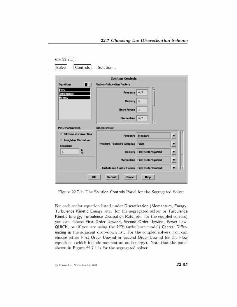
22.7 Choosing the Discretization Scheme
ure 22.7.1).
Solve −→ Controls −→Solution...
Figure 22.7.1: The Solution Controls Panel for the Segregated Solver
For each scalar equation listed under Discretization (Momentum, Energy,Turbulence Kinetic Energy, etc. for the segregated solver or TurbulenceKinetic Energy, Turbulence Dissipation Rate, etc. for the coupled solvers)you can choose First Order Upwind, Second Order Upwind, Power Law,QUICK, or (if you are using the LES turbulence model) Central Differ-encing in the adjacent drop-down list. For the coupled solvers, you canchoose either First Order Upwind or Second Order Upwind for the Flowequations (which include momentum and energy). Note that the panelshown in Figure 22.7.1 is for the segregated solver.
c© Fluent Inc. November 28, 2001 22-55

Using the Solver
If you are using the segregated solver, select the pressure interpola-tion scheme under Discretization in the drop-down list next to Pressure.You can choose Standard, Linear, Second Order, Body Force Weighted,or PRESTO!. If you are using the segregated solver and your flow iscompressible (i.e., you are using the ideal gas law for density), selectthe density interpolation scheme under Discretization in the drop-downlist next to Density. You can choose First Order Upwind, Second OrderUpwind, or QUICK. (Note that Density will not appear for incompressibleor multiphase flows.)
If you change the settings for Discretization, but you then want to returnto FLUENT’s default settings, you can click on the Default button. FLU-ENT will change the settings to the defaults and the Default button willbecome the Reset button. To get your settings back again, you can clickon the Reset button.
22.8 Choosing the Pressure-Velocity Coupling Method
FLUENT provides three methods for pressure-velocity coupling in thesegregated solver: SIMPLE, SIMPLEC, and PISO. Steady-state calcu-lations will generally use SIMPLE or SIMPLEC, while PISO is recom-mended for transient calculations. PISO may also be useful for steady-state and transient calculations on highly skewed meshes.
Pressure-velocity coupling is relevant only for the segregated solver; you!will not specify it for the coupled solvers.
22.8.1 SIMPLE vs. SIMPLEC
In FLUENT, both the standard SIMPLE algorithm and the SIMPLEC(SIMPLE-Consistent) algorithm are available. SIMPLE is the default,but many problems will benefit from the use of SIMPLEC, particularlybecause of the increased under-relaxation that can be applied, as de-scribed below.
For relatively uncomplicated problems (laminar flows with no additionalmodels activated) in which convergence is limited by the pressure-velocitycoupling, you can often obtain a converged solution more quickly usingSIMPLEC. With SIMPLEC, the pressure-correction under-relaxation
22-56 c© Fluent Inc. November 28, 2001

22.8 Choosing the Pressure-Velocity Coupling Method
factor is generally set to 1.0, which aids in convergence speed-up. In someproblems, however, increasing the pressure-correction under-relaxationto 1.0 can lead to instability. For such cases, you will need to use amore conservative under-relaxation value or use the SIMPLE algorithm.For complicated flows involving turbulence and/or additional physicalmodels, SIMPLEC will improve convergence only if it is being limitedby the pressure-velocity coupling. Often it will be one of the additionalmodeling parameters that limits convergence; in this case, SIMPLE andSIMPLEC will give similar convergence rates.
22.8.2 PISO
The PISO algorithm (see Section 22.3.3) with neighbor correction ishighly recommended for all transient flow calculations, especially whenyou want to use a large time step. (For problems that use the LESturbulence model, which usually requires small time steps, using PISOmay result in increased computational expense, so SIMPLE or SIMPLECshould be considered instead.) PISO can maintain a stable calculationwith a larger time step and an under-relaxation factor of 1.0 for bothmomentum and pressure. For steady-state problems, PISO with neigh-bor correction does not provide any noticeable advantage over SIMPLEor SIMPLEC with optimal under-relaxation factors.
PISO with skewness correction is recommended for both steady-stateand transient calculations on meshes with a high degree of distortion.
When you use PISO neighbor correction, under-relaxation factors of 1.0or near 1.0 are recommended for all equations. If you use just the PISOskewness correction for highly-distorted meshes, set the under-relaxationfactors for momentum and pressure so that they sum to 1 (e.g., 0.3 forpressure and 0.7 for momentum). If you use both PISO methods, fol-low the under-relaxation recommendations for PISO neighbor correction,above.
22.8.3 User Inputs
You can specify the pressure-velocity coupling method in the SolutionControls panel (Figure 22.7.1).
c© Fluent Inc. November 28, 2001 22-57

Using the Solver
Solve −→ Controls −→Solution...
Choose SIMPLE, SIMPLEC, or PISO in the Pressure-Velocity Couplingdrop-down list under Discretization.
If you choose PISO, the panel will expand to show the PISO Parameters.By default, both Skewness Correction and Neighbor Correction are on. Ifyou want to use just neighbor correction or just skewness correction, youcan turn off the appropriate option. The default number of Iterations isset to 1; you should not need to change this value.
22.9 Setting Under-Relaxation Factors
As discussed in Section 22.2.7, the segregated solver uses under-relaxationto control the update of computed variables at each iteration. Thismeans that all equations solved using the segregated solver, includingthe non-coupled equations solved by the coupled solvers (turbulence andother scalars, as discussed in Section 22.1.2), will have under-relaxationfactors associated with them.
In FLUENT, the default under-relaxation parameters for all variables areset to values that are near optimal for the largest possible number ofcases. These values are suitable for many problems, but for some partic-ularly nonlinear problems (e.g., some turbulent flows or high-Rayleigh-number natural-convection problems) it is prudent to reduce the under-relaxation factors initially.
It is good practice to begin a calculation using the default under-relaxationfactors. If the residuals continue to increase after the first 4 or 5 itera-tions, you should reduce the under-relaxation factors.
Occasionally, you may make changes in the under-relaxation factors andresume your calculation, only to find that the residuals begin to increase.This often results from increasing the under-relaxation factors too much.A cautious approach is to save a data file before making any changes tothe under-relaxation factors, and to give the solution algorithm a fewiterations to adjust to the new parameters. Typically, an increase in theunder-relaxation factors brings about a slight increase in the residuals,but these increases usually disappear as the solution progresses. If the
22-58 c© Fluent Inc. November 28, 2001
22.9 Setting Under-Relaxation Factors
residuals jump by a few orders of magnitude, you should consider haltingthe calculation and returning to the last good data file saved.
Note that viscosity and density are under-relaxed from iteration to it-eration. Also, if the enthalpy equation is solved directly instead of thetemperature equation (i.e., for non-premixed combustion calculations),the update of temperature based on enthalpy will be under-relaxed. Tosee the default under-relaxation factors, you can click on the Defaultbutton in the Solution Controls panel.
For most flows, the default under-relaxation factors do not usually re-quire modification. If unstable or divergent behavior is observed, how-ever, you need to reduce the under-relaxation factors for pressure, mo-mentum, k, and ε from their default values to about 0.2, 0.5, 0.5, and0.5. (It is usually not necessary to reduce the pressure under-relaxationfor SIMPLEC.) In problems where density is strongly coupled with tem-perature, as in very-high-Rayleigh-number natural- or mixed-convectionflows, it is wise to also under-relax the temperature equation and/or den-sity (i.e., use an under-relaxation factor less than 1.0). Conversely, whentemperature is not coupled with the momentum equations (or when it isweakly coupled), as in flows with constant density, the under-relaxationfactor for temperature can be set to 1.0.
For other scalar equations (e.g., swirl, species, mixture fraction and vari-ance) the default under-relaxation may be too aggressive for some prob-lems, especially at the start of the calculation. You may wish to reducethe factors to 0.8 to facilitate convergence.
User Inputs
You can modify the under-relaxation factors in the Solution Controlspanel (Figure 22.7.1).
Solve −→ Controls −→Solution...
You can set the under-relaxation factor for each equation in the fieldnext to its name under Under-Relaxation Factors.
If you are using the segregated solver, all equations will have an associ-!ated under-relaxation factor. If you are using one of the coupled solvers,
c© Fluent Inc. November 28, 2001 22-59
Using the Solver
only those equations that are solved sequentially (see Section 22.1.2) willhave under-relaxation factors.
If you change under-relaxation factors, but you then want to return toFLUENT’s default settings, you can click on the Default button. FLUENTwill change the factors to the default values and the Default button willbecome the Reset button. To get your settings back again, you can clickon the Reset button.
22.10 Changing the Courant Number
For FLUENT’s coupled solvers, the main control over the time-steppingscheme is the Courant number (CFL). The time step is proportional tothe CFL, as defined in Equation 22.4-13.
Linear stability theory determines a range of permissible values for theCFL (i.e., the range of values for which a given numerical scheme willremain stable). When you specify a permissible CFL value, FLUENT willcompute an appropriate time step using Equation 22.4-13. In general,taking larger time steps leads to faster convergence, so it is advantageousto set the CFL as large as possible (within the permissible range).
The stability limits of the coupled implicit and explicit solvers are signifi-cantly different. The explicit solver has a more limited range and requireslower CFL settings than does the coupled implicit solver. Appropriatechoices of CFL for the two solvers are discussed below.
22.10.1 Courant Numbers for the Coupled Explicit Solver
Linear stability analysis shows that the maximum allowable CFL for themulti-stage scheme used in the coupled explicit solver will depend on thenumber of stages used and how often the dissipation and viscous termsare updated (see Section 22.19.5). But in general, you can assume thatthe multi-stage scheme is stable for Courant numbers up to 2.5. Thisstability limit is often lower in practice because of nonlinearities in thegoverning equations.
The default CFL for the coupled explicit solver is 1.0, but you may beable to increase it for some 2D problems. You should generally not use
22-60 c© Fluent Inc. November 28, 2001

22.10 Changing the Courant Number
a value higher than 2.0.
If your solution is diverging, i.e., if residuals are rising very rapidly, andyour problem is properly set up and initialized, this is usually a goodsign that the Courant number needs to be lowered. Depending on theseverity of the startup conditions, you may need to decrease the CFL toa value as low as 0.1 to 0.5 to get started. Once the startup transientsare reduced you can start increasing the Courant number again.
22.10.2 Courant Numbers for the Coupled Implicit Solver
Linear stability theory shows that the point Gauss-Seidel scheme used inthe coupled implicit solver is unconditionally stable. However, as withthe explicit solver, nonlinearities in the governing equations will oftenlimit stability.
The default CFL for the coupled implicit solver is 5.0. It is often possibleto increase the CFL to 10, 20, 100, or even higher, depending on thecomplexity of your problem. You may find that a lower CFL is requiredduring startup (when changes in the solution are highly nonlinear), butit can be increased as the solution progresses.
The coupled AMG solver has the capability to detect divergence of themultigrid cycles within a given iteration. If this happens, it will auto-matically reduce the CFL and perform the iteration again, and a messagewill be printed to the screen. Five attempts are made to complete theiteration successfully. Upon successful completion of the current itera-tion the CFL is returned to its original value and the iteration procedureproceeds as required.
22.10.3 User Inputs
The Courant number is set in the Solution Controls panel (Figure 22.10.1).
Solve −→ Controls −→Solution...
Enter the value for Courant Number under Solver Parameters. (Note thatthe panel shown in Figure 22.10.1 is for the coupled explicit solver. Forthe coupled implicit solver, the Courant Number is the only item thatwill appear under Solver Parameters.)
c© Fluent Inc. November 28, 2001 22-61

Using the Solver
Figure 22.10.1: The Solution Controls Panel for the Coupled ExplicitSolver
When you select the coupled explicit solver in the Solver panel, FLU-ENT will automatically set the Courant Number to 1; when you selectthe coupled implicit solver, the Courant Number will be changed to 5automatically.
22-62 c© Fluent Inc. November 28, 2001

22.11 Turning On FAS Multigrid
22.11 Turning On FAS Multigrid
As discussed in Section 22.5, FAS multigrid is an optional component ofthe coupled explicit solver. (AMG multigrid is always on, by default.)Since nearly all coupled explicit calculations will benefit from the use ofthe FAS multigrid convergence accelerator, you should generally set anon-zero number of coarse grid levels before beginning the calculation.For most problems, this will be the only FAS multigrid parameter youwill need to set. Should you encounter convergence difficulties, considerapplying one of the methods discussed in Section 22.19.4.
Note that you cannot use FAS multigrid with explicit time stepping!(described in Section 22.2.8) because the coarse grid corrections willdestroy the time accuracy of the fine grid solution.
22.11.1 Setting Coarse Grid Levels
As discussed in Section 22.5.4, FAS multigrid solves on successivelycoarser grids and then transfers corrections to the solution back up tothe original fine grid, thus increasing the propagation speed of the solu-tion and speeding convergence. The most basic way you can control themultigrid solver is by specifying the number of coarse grid levels to beused.
As explained in Section 22.5.4, the coarse grid levels are formed by ag-glomerating a group of adjacent “fine” cells into a single “coarse” cell.The optimal number of grid levels is therefore problem-dependent. Formost problems, you can start out with 4 or 5 levels. For large 3D prob-lems, you may want to add more levels (although memory restrictionsmay prevent you from using more levels, since each coarse grid levelrequires additional memory). If you believe that multigrid is causingconvergence trouble, you can decrease the number of levels.
If FLUENT reaches a coarse grid with one cell before creating as manylevels as you requested, it will simply stop there. That is, if you request5 levels, and level 4 has only 1 cell, FLUENT will create only 4 levels,since levels 4 and 5 would be the same.
To specify the number of grid levels you want, set the number of Multi-grid Levels in the Solution Controls panel (Figure 22.10.1) under Solver
c© Fluent Inc. November 28, 2001 22-63
Using the Solver
Parameters.
Solve −→ Controls −→Solution...
You can also set the Max Coarse Levels under FAS Multigrid Controls inthe Multigrid Controls panel.
Solve −→ Controls −→Multigrid...
Changing the number of coarse grid levels in one panel will automaticallyupdate the number shown in the other.
Coarse grid levels are created when you first begin iterating. If youwant to check how many cells are in each level, request one iterationand then use the Grid/Info/Size menu item (described in Section 5.6.1)to list the size of each grid level. If you are satisfied, you can continuethe calculation; if not, you can change the number of coarse grid levelsand check again.
For most problems, you will not need to modify any additional multigridparameters once you have settled on an appropriate number of coarsegrid levels. You can simply continue your calculation until convergence.
22.12 Setting Solution Limits
In order to keep the solution stable under extreme conditions, FLUENTprovides limits that keep the solution within an acceptable range. Youcan control these limits with the Solution Limits panel (Figure 22.12.1).
Solve −→ Controls −→Limits...
FLUENT applies limiting values for pressure, temperature, and turbu-lence quantities. The purpose of these limits is to keep the absolutepressure or the temperature from becoming 0, negative, or excessivelylarge during the calculation, and to keep the turbulence quantities frombecoming excessive. FLUENT also puts a limit on the rate of reductionof temperature to prevent it from becoming 0 or negative.
Typically, you will not need to change the default solution limits. If pres-!sure, temperature, or turbulence quantities are being reset to the limitingvalue repeatedly (as indicated by the appropriate warning messages in
22-64 c© Fluent Inc. November 28, 2001

22.12 Setting Solution Limits
Figure 22.12.1: The Solution Limits Panel
the console window), you should check the dimensions, boundary condi-tions, and properties to be sure that the problem is set up correctly andtry to determine why the variable in question is getting so close to zeroor so large. You can use the “marking” feature (used to mark cells foradaption) to identify which cells have a value equal to the limit. (Usethe Iso-Value Adaption panel, as described in Section 23.5.) In very rarecases, you may need to change the solution limits, but only do so if youare sure that you understand the reason for the solver’s unusual behav-ior. (For example, you may know that the temperature in your domainwill exceed 5000 K. Be sure that any temperature-dependent proper-ties are appropriately defined for high temperatures if you increase themaximum temperature limit.)
Limiting the Values of Solution Variables
The limiting minimum and maximum values for absolute pressure areshown in the Minimum and Maximum Absolute Pressure fields. If the FLU-ENT calculation predicts a value less than the Minimum Absolute Pressure
c© Fluent Inc. November 28, 2001 22-65
Using the Solver
or greater than the Maximum Absolute Pressure, the corresponding lim-iting value will be used instead. Similarly, the Minimum and MaximumTemperature are limiting values for energy calculations.
The Maximum Turb. Viscosity Ratio and the Minimum Turb. KineticEnergy are limiting values for turbulent calculations. If the calculationpredicts a k value less than the Minimum Turb. Kinetic Energy, the lim-iting value will be used instead. For the viscosity ratio limit, FLUENTuses the limiting maximum value of turbulent viscosity (Cµk
2/ε) in theflow field relative to the laminar viscosity. If the ratio calculated byFLUENT exceeds the limiting value, the ratio is set to the limiting valueby limiting ε to the necessary value.
Limiting the Reduction Rate for Temperature
In FLUENT’s coupled solvers, the rate of reduction of temperature is con-trolled by the Positivity Rate Limit. The default value of 0.2, for example,means that temperature is not allowed to decrease by more than 20%of its previous value from one iteration to the next. If the temperaturechange exceeds this limit, the time step in that cell is reduced to bringthe change back into range and a “time step reduced” warning is printed.(This reduced time step will be used for the solution of all variables inthe cell, not just for temperature.) Rapid reduction of temperature is anindication that the temperature may become negative. Repeated “timestep reduced” warnings should alert you that something is wrong in yourproblem setup. (If the warning messages stop appearing, the calculationmay have “recovered” from the time-step reduction.)
Resetting Solution Limits
If you change and save the value of one of the solution limits, but youthen want to return to the default limits set by FLUENT, you can reopenthe Solution Limits panel and click on the Default button. FLUENT willchange the values to the defaults and the Default button will become theReset button. To get your values back again, you can click on the Resetbutton.
22-66 c© Fluent Inc. November 28, 2001

22.13 Initializing the Solution
22.13 Initializing the Solution
Before starting your CFD simulation, you must provide FLUENT with aninitial “guess” for the solution flow field. In many cases, you must takeextra care to provide an initial solution that will allow the desired finalsolution to be attained. A real-life supersonic wind tunnel, for example,will not “start” if the back pressure is simply lowered to its operatingvalue; the flow will choke at the tunnel throat and will not transitionto supersonic. The same holds true for a numerical simulation: the flowmust be initialized to a supersonic flow or it will simply choke and remainsubsonic.
There are two methods for initializing the solution:
• Initialize the entire flow field (in all cells).
• Patch values or functions for selected flow variables in selected cellzones or “registers” of cells. (Registers are created with the samefunctions that are used to mark cells for adaption.)
Before patching initial values in selected cells, you must first initialize the!entire flow field. You can then patch the new values over the initializedvalues for selected variables.
22.13.1 Initializing the Entire Flow Field
Before you start your calculations or patch initial values for selected vari-ables in selected cells (Section 22.13.2) you must initialize the flow fieldin the entire domain. The Solution Initialization panel (Figure 22.13.1)allows you to set initial values for the flow variables and initialize thesolution using these values.
Solve −→ Initialize −→Initialize...
You can compute the values from information in a specified zone, enterthem manually, or have the solver compute average values based on allzones. You can also indicate whether the specified values for velocitiesare absolute or relative to the velocity in each cell zone. The steps forinitialization are as follows:
c© Fluent Inc. November 28, 2001 22-67
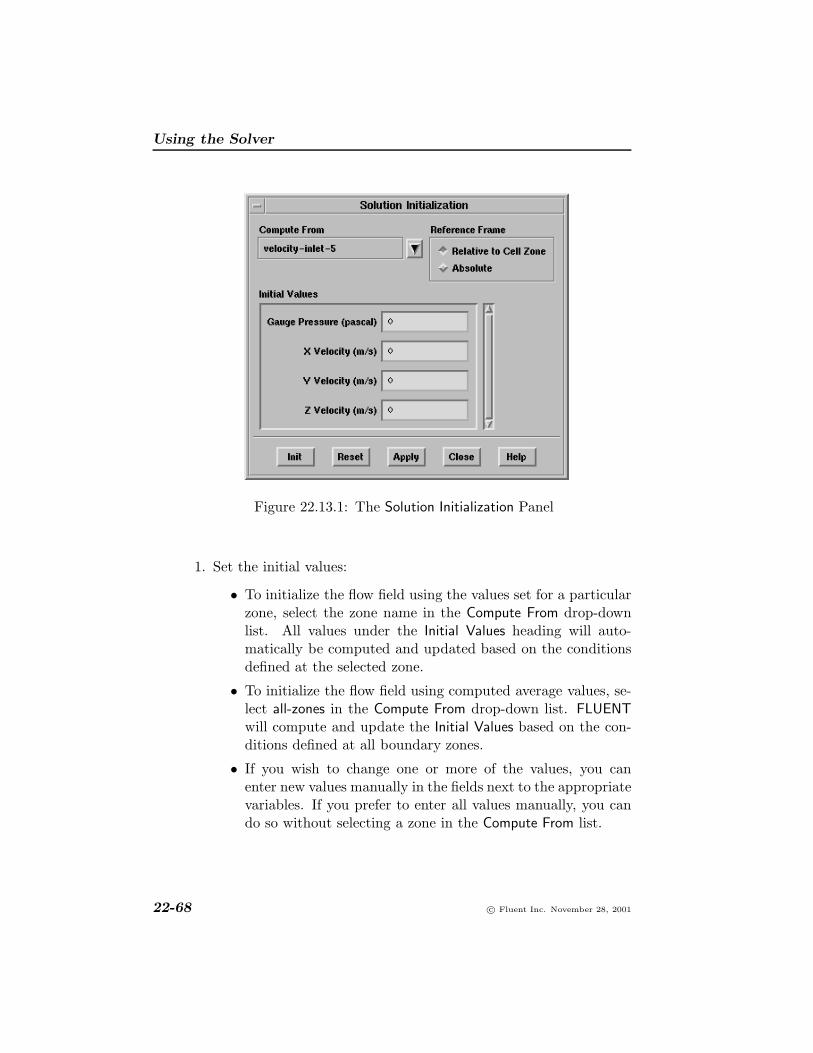
Using the Solver
Figure 22.13.1: The Solution Initialization Panel
1. Set the initial values:
• To initialize the flow field using the values set for a particularzone, select the zone name in the Compute From drop-downlist. All values under the Initial Values heading will auto-matically be computed and updated based on the conditionsdefined at the selected zone.
• To initialize the flow field using computed average values, se-lect all-zones in the Compute From drop-down list. FLUENTwill compute and update the Initial Values based on the con-ditions defined at all boundary zones.
• If you wish to change one or more of the values, you canenter new values manually in the fields next to the appropriatevariables. If you prefer to enter all values manually, you cando so without selecting a zone in the Compute From list.
22-68 c© Fluent Inc. November 28, 2001

22.13 Initializing the Solution
2. If your problem involves moving reference frames or sliding meshes,indicate whether the initial velocities are absolute velocities or ve-locities relative to the motion of each cell zone by selecting Absoluteor Relative to Cell Zone under Reference Frame. (If no zone motionoccurs in the problem, the two options are equivalent.) The defaultreference frame for velocity initialization in FLUENT is relative. Ifthe solution in most of your domain is rotating, using the relativeoption may be better than using the absolute option.
3. Once you are satisfied with the Initial Values displayed in the panel,you can click on the Init button to initialize the flow field. If so-lution data already exist (i.e., if you have already performed somecalculations or initialized the solution), you must confirm that itis OK to overwrite those data.
Saving and Resetting Initial Values
When you initialize the solution by clicking on Init, the initial valueswill also be saved; should you need to reinitialize the solution later, youwill find the correct values in the panel when you reopen it. If you wishto define initial values now, but you are not yet ready to initialize thesolution, you can follow the instructions above for setting the values andthen click Apply instead of Init. This will save the currently displayedvalues without initializing the solution. You can return to the panel lateron and perform the initialization.
If you accidentally select the wrong zone from the Compute From list ormanually set a value incorrectly, you can use the Reset button to resetall fields to their “saved” values. Values are saved each time the panelis opened, before Compute From is executed, and after Init or Apply isexecuted.
c© Fluent Inc. November 28, 2001 22-69

Using the Solver
22.13.2 Patching Values in Selected Cells
Once you have initialized (or calculated) the entire flow field, you maypatch different values for particular variables into different cells. If youhave multiple fluid zones, for example, you may want to patch a differenttemperature in each one. You can also choose to patch a custom fieldfunction (defined using the Custom Field Function Calculator panel) in-stead of a constant value. If you are patching velocities, you can indicatewhether the specified values are absolute velocities or velocities relativeto the cell zone’s velocity. All patching operations are performed withthe Patch panel (Figure 22.13.2).
Solve −→ Initialize −→Patch...
Figure 22.13.2: The Patch Panel
1. Select the variable to be patched in the Variable list.
2. In the Zones To Patch and/or Registers To Patch lists, choose thezone(s) and/or register(s) for which you want to patch a value forthe selected variable.
22-70 c© Fluent Inc. November 28, 2001

22.13 Initializing the Solution
3. If you wish to patch a constant value, simply enter that value in theValue field. If you want to patch a previously-defined field function,turn on the Use Field Function option and select the appropriatefunction in the Field Function list.
4. If you selected a velocity in the Variable list, and your problem in-volves moving reference frames or sliding meshes, indicate whetherthe patched velocities are absolute velocities or velocities relativeto the motion of each cell zone by selecting Absolute or Relative toCell Zone under Reference Frame. (If no zone motion occurs in theproblem, the two options are equivalent.) The default referenceframe for velocity patching in FLUENT is relative. If the solutionin most of your domain is rotating, using the relative option maybe better than using the absolute option.
5. Click on the Patch button to update the flow-field data. (Note thatpatching will have no effect on the iteration or time-step count.)
Using Registers
The ability to patch values in cell registers gives you the flexibility topatch different values within a single cell zone. For example, you maywant to patch a certain value for temperature only in fluid cells witha particular range of concentrations for one species. You can create acell register (basically a list of cells) using the functions that are used tomark cells for adaption. These functions allow you to mark cells basedon physical location, cell volume, gradient or isovalue of a particularvariable, and other parameters. See Chapter 23 for information aboutmarking cells for adaption. Section 23.9 provides information about ma-nipulating different registers to create new ones. Once you have createda register, you can patch values in it as described above.
Using Field Functions
By defining your own field function using the Custom Field Function Cal-culator panel, you can patch a non-constant value in selected cells. Forexample, you may want to patch varying species mass fractions through-out a fluid region. To use this feature, simply create the function as
c© Fluent Inc. November 28, 2001 22-71

Using the Solver
described in Section 27.5, and then perform the function-patching oper-ation in the Patch panel, as described above.
Using Patching Later in the Solution Process
Since patching affects only the variables for which you choose to changethe value, leaving the rest of the flow field intact, you can use it later inthe solution process without losing calculated data. (Initialization, onthe other hand, resets all data to the initial values.) For example, youmight want to start a combustion calculation from a cold-flow solution.You can simply read in (or calculate) the cold-flow data, patch a hightemperature in the appropriate cells, and continue the calculation.
Patching can also be useful when you are solving a problem using astep-by-step technique, as described in Section 22.19.2.
22-72 c© Fluent Inc. November 28, 2001

22.14 Performing Steady-State Calculations
22.14 Performing Steady-State Calculations
For steady-state calculations, you will request the start of the solutionprocess using the Iterate panel (Figure 22.14.1).
Solve −→Iterate...
Figure 22.14.1: The Iterate Panel
In this panel, you will supply the number of additional iterations to beperformed in the Number of Iterations field. (For unsteady calculationinputs, see Section 22.15.1.) If no calculations have been performed yet,FLUENT will begin calculations starting at iteration 1, using the initialsolution. If you are starting from current solution data, FLUENT willbegin at the last iteration performed, using the current solution data asits starting point.
By default, FLUENT will update the convergence monitors (described inSection 22.16) after each iteration. If you increase the Reporting Intervalfrom the default of 1 you can get reports less frequently. For example,if you set the Reporting Interval to 2, the monitors will print or plotreports at every other iteration. Note that the Reporting Interval alsospecifies how often FLUENT should check if the solution is converged.For example, if your solution converges after 40 iterations, but yourReporting Interval is set to 50, FLUENT will continue the calculation foran extra 10 iterations before checking for (and finding) convergence.
c© Fluent Inc. November 28, 2001 22-73

Using the Solver
When you click on the Iterate button, FLUENT will begin to calculate.During iteration, a Working dialog is displayed. Clicking on the Cancelbutton or typing <Control-C> in the FLUENT console window will in-terrupt the iteration, as soon as it is safe to stop. (See below for moredetails.)
Updating UDF Profiles
If you have used a user-defined function (UDF) to define any boundaryconditions, properties, etc., you can control the frequency with which thefunction is updated by modifying the value of the UDF Profile UpdateInterval. If UDF Profile Update Interval is set to n, the function will beupdated after every n iterations.
By default, the UDF Profile Update Interval is set to 1. You might wantto increase this value if your profile computation is expensive. See theseparate UDF Manual for details about creating and using UDFs.
Interrupting Iterations
As mentioned above, you can interrupt the calculation by clicking on theCancel button in the Working dialog box that appears while the solveris calculating. In addition, on most, but not all, computer systems youwill be able to interrupt calculations using a control sequence, usually<Control-C>. This allows you to stop the calculation process beforeproceeding with the remainder of the requested iterations.
Resetting Data
After you have performed some iterations, if you decide to start overagain from the first iteration (e.g., after making some changes to theproblem setup), you can reinitialize the solution using the Solution Ini-tialization panel, as described in Section 22.13.1.
22-74 c© Fluent Inc. November 28, 2001

22.15 Performing Time-Dependent Calculations
22.15 Performing Time-Dependent Calculations
FLUENT can solve the conservation equations in time-dependent form,to simulate a wide variety of time-dependent phenomena, such as
• vortex shedding and other time-periodic phenomena
• compressible filling and emptying problems
• transient heat conduction
• transient chemical mixing and reactions
Figures 22.15.1 and 22.15.2 illustrate the time-dependent vortex shed-ding flow pattern in the wake of a cylinder.
Activating time dependence is sometimes useful when attempting tosolve steady-state problems which tend toward instability (e.g., natu-ral convection problems in which the Rayleigh number is close to thetransition region). It is possible in many cases to reach a steady-statesolution by integrating the time-dependent equations.
See Section 22.2.8 for details about temporal discretization.
22.15.1 User Inputs for Time-Dependent Problems
To solve a time-dependent problem, you will follow the procedure out-lined below:
1. Enable the Unsteady option in the Solver panel (Figure 22.15.3),and specify the desired Unsteady Formulation.
Define −→ Models −→Solver...
The 1st-Order Implicit formulation is sufficient for most problems.If you need improved accuracy, you can use the 2nd-Order Implicitformulation instead. The Explicit formulation (available only if thecoupled explicit solver is selected under Solver and Formulation atthe top of the panel) is used primarily to capture the transientbehavior of moving waves, such as shocks. See Section 22.2.8 fordetails.
c© Fluent Inc. November 28, 2001 22-75

Using the Solver
Contours of Stream Function (kg/s) (Time=3.6600e+01)
1.92e+01
1.76e+01
1.60e+01
1.44e+01
1.28e+01
1.12e+01
9.60e+00
8.00e+00
6.40e+00
4.80e+00
3.20e+00
1.60e+00
0.00e+00
Figure 22.15.1: Time-Dependent Calculation of Vortex Shedding (t=3.66sec)
Contours of Stream Function (kg/s) (Time=4.1600e+01)
1.92e+01
1.76e+01
1.60e+01
1.44e+01
1.28e+01
1.12e+01
9.60e+00
8.00e+00
6.40e+00
4.80e+00
3.20e+00
1.60e+00
0.00e+00
Figure 22.15.2: Time-Dependent Calculation of Vortex Shedding (t=41.6sec)
22-76 c© Fluent Inc. November 28, 2001

22.15 Performing Time-Dependent Calculations
Figure 22.15.3: The Solver Panel for an Unsteady Calculation
2. Define all relevant models and boundary conditions. Note that anyboundary conditions specified using user-defined functions can bemade to vary in time. See the separate UDF Manual for details.
3. If you are using the segregated solver, choose PISO as the Pressure-Velocity Coupling scheme under Discretization in the Solution Con-trols panel.
Solve −→ Controls −→Solution...
In general, you will not need to modify the PISO Parameters fromtheir default values. See Section 22.8.2 for more information aboutusing the PISO algorithm.
If you are using the LES turbulence model with small time steps,!the PISO scheme may be too computationally expensive. It istherefore recommended that you use SIMPLE or SIMPLEC insteadof PISO.
c© Fluent Inc. November 28, 2001 22-77

Using the Solver
4. (optional) If you are using the explicit unsteady formulation or ifyou are using the adaptive time stepping method (described be-low and in Section 22.15.2) it is recommended that you enable theprinting of the current time (for the explicit unsteady formula-tion) or the current time step size (for the adaptive time steppingmethod) at each iteration, using the Statistic Monitors panel.
Solve −→ Monitors −→Statistic...
Select time (for the current time) or delta time (for the currenttime step size) in the Statistics list and turn on the Print option.When FLUENT prints the residuals to the console window at eachiteration, it will include a column with the current time or thecurrent time step size.
5. (optional) Use the Force Monitors panel or the Surface Monitorspanel to monitor (and/or save to a file) time-varying force coef-ficient values or the average, mass average, integral, or flux of afield variable or function on a surface as it changes with time. SeeSection 22.16 for details.
6. Set the initial conditions (at time t = 0) using the Solution Initial-ization panel.
Solve −→ Initialize −→Initialize...
You can also read in a steady-state data file to set the initial con-ditions.
File −→ Read −→Data...
7. Use the automatic saving feature to specify the file name and fre-quency with which case and data files should be saved during thesolution process.
File −→ Write −→Autosave...
See Section 3.3.4 for details about the use of this feature.
You may also want to request automatic execution of other com-mands using the Execute Commands panel. See Section 22.18 fordetails.
22-78 c© Fluent Inc. November 28, 2001
22.15 Performing Time-Dependent Calculations
8. (optional) If you want to create a graphical animation of the solu-tion over time, you can use the Solution Animation panel to set upthe graphical displays that you want to use in the animation. SeeSection 22.17 for details.
9. (optional) If you want FLUENT to gather data for time statistics(i.e., time-averaged and root-mean-square values for solution vari-ables) during the calculation, follow these steps:
(a) Turn on the Data Sampling for Time Statistics option in theIterate panel.
Solve −→Iterate...
Enabling this option will allow you to display and reportboth the mean and the root-mean-square (RMS) values, asdescribed in Section 22.15.3.
Note that gathering data for time statistics is not meaningful!inside a moving cell zone (i.e., a sliding zone in a sliding meshproblem).
(b) Initialize the flow statistics.
solve −→ initialize −→init-flow-statistics
Note that you can also use the init-flow-statistics textcommand to reset the flow statistics after you have gatheredsome data for time statistics. If you perform, say, 10 timesteps with the Data Sampling for Time Statistics option en-abled, check the results, and then continue the calculation for10 more time steps, the time statistics will include the datagathered in the first 10 time steps unless you reinitialize theflow statistics.
10. Specify time-dependent solution parameters and start the calcu-lation, as described below for the implicit and explicit unsteadyformulations:
• If you have chosen the 1st-Order or 2nd-Order Implicit formu-lation, the procedure is as follows:
(a) Set the time-dependent solution parameters in the Iteratepanel (Figure 22.15.4).
c© Fluent Inc. November 28, 2001 22-79
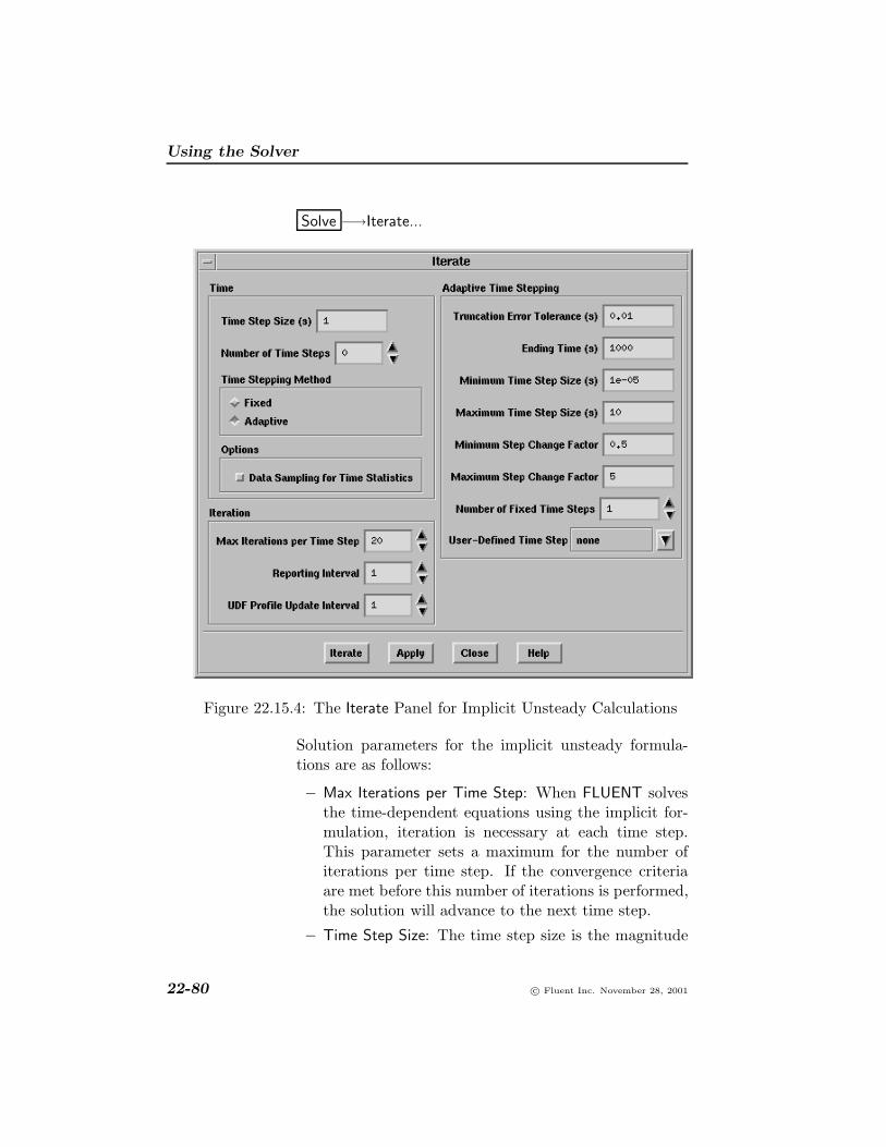
Using the Solver
Solve −→Iterate...
Figure 22.15.4: The Iterate Panel for Implicit Unsteady Calculations
Solution parameters for the implicit unsteady formula-tions are as follows:
– Max Iterations per Time Step: When FLUENT solvesthe time-dependent equations using the implicit for-mulation, iteration is necessary at each time step.This parameter sets a maximum for the number ofiterations per time step. If the convergence criteriaare met before this number of iterations is performed,the solution will advance to the next time step.
– Time Step Size: The time step size is the magnitude
22-80 c© Fluent Inc. November 28, 2001

22.15 Performing Time-Dependent Calculations
of ∆t. Since the FLUENT formulation is fully im-plicit, there is no stability criterion that needs to bemet in determining ∆t. However, to model transientphenomena properly, it is necessary to set ∆t at leastone order of magnitude smaller than the smallest timeconstant in the system being modeled. A good wayto judge the choice of ∆t is to observe the numberof iterations FLUENT needs to converge at each timestep. The ideal number of iterations per time step is10–20. If FLUENT needs substantially more, the timestep is too large. If FLUENT needs only a few itera-tions per time step, ∆t may be increased. Frequentlya time-dependent problem has a very fast “startup”transient that decays rapidly. It is thus often wiseto choose a conservatively small ∆t for the first 5–10time steps. ∆t may then be gradually increased asthe calculation proceeds.
For time-periodic calculations, you should choose thetime step based on the time scale of the periodic-ity. For a rotor/stator model, for example, you mightwant 20 time steps between each blade passing. Forvortex shedding, you might want 20 steps per period.
By default, the size of the time step is fixed (as indicatedby the selection of Fixed under Time Stepping Method).To have FLUENT modify the size of the time step as thecalculation proceeds, select Adaptive and specify the pa-rameters under Adaptive Time Stepping in the expandedIterate panel. See Section 22.15.2 for details.
With the Adaptive time stepping method, the value youspecify for the Time Step Size will be the initial size of thetime step. As the calculation proceeds, the Time Step Sizeshown in the Iterate panel will be the size of the currenttime step.
(b) Specify the desired Number of Time Steps in the Iteratepanel and click Iterate.
c© Fluent Inc. November 28, 2001 22-81

Using the Solver
As it calculates a solution, FLUENT will print the currenttime at the end of each time step.
• If you have chosen the Explicit unsteady formulation, you willfollow a different procedure:
(a) Use the default settings for the Solver Parameters in theSolution Controls panel.
Solve −→ Controls −→Solution...
If you have modified the Solver Parameters, you can clickon the Default button to retrieve the default settings.
(b) Specify the desired Number of Iterations and click Iterate.
Solve −→Iterate...
Remember that when the explicit unsteady formulationis used, each iteration is a time step. When FLUENTprints the residuals to the console window, it will includea column with the current time (if you requested this instep 4, above).
11. Save the final data file (and case file, if you have modified it) sothat you can continue the unsteady calculation later, if desired.
File −→ Write −→Data...
Additional Inputs
The procedures for setting the reporting interval, updating UDF pro-files, interrupting iterations, and resetting data are the same as those forsteady-state calculations. See Section 22.14 for details.
If you are using a user-defined function in your time-dependent calcu-!lation, note that, in addition to being updated after every n iterations(where n is the value of the UDF Profile Update Interval), the functionwill also be updated at the first iteration of each time step.
22-82 c© Fluent Inc. November 28, 2001
22.15 Performing Time-Dependent Calculations
22.15.2 Adaptive Time Stepping
As mentioned in Section 22.15.1, it is possible to have the size of the timestep change as the calculation proceeds, rather than specifying a fixedsize for the entire calculation. This section provides a brief description ofthe algorithm that FLUENT uses to compute the time step size, as wellas an explanation of each of the parameters that you can set to controlthe adaptive time stepping.
Adaptive time stepping is available only with the segregated and coupled!implicit solvers; it cannot be used with the coupled explicit solver. Inaddition, it cannot be used with the VOF or discrete phase model.
The Adaptive Time Stepping Algorithm
The automatic determination of the time step size is based on the estima-tion of the truncation error associated with the time integration scheme(i.e., first-order implicit or second-order implicit). If the truncation erroris smaller than a specified tolerance, the size of the time step is increased;if the truncation error is greater, the time step size is decreased.
An estimation of the truncation error can be obtained by using a predictor-corrector type of algorithm [82] in association with the time integrationscheme. At each time step, a predicted solution can be obtained us-ing a computationally inexpensive explicit method (forward Euler forthe first-order unsteady formulation, Adams-Bashford for the second-order unsteady formulation). This predicted solution is used as an ini-tial condition for the time step, and the correction is computed usingthe non-linear iterations associated with the implicit (segregated or cou-pled) algorithm. The norm of the difference between the predicted andcorrected solutions is used as a measure of the truncation error. By com-paring the truncation error with the desired level of accuracy (i.e., thetruncation error tolerance), FLUENT is able to adjust the time step sizeby increasing it or decreasing it.
Specifying Parameters for Adaptive Time Stepping
The parameters that control the adaptive time stepping appear in theIterate panel, as described in Section 22.15.1. These parameters are as
c© Fluent Inc. November 28, 2001 22-83

Using the Solver
follows:
Truncation Error Tolerance specifies the threshold value to which the com-puted truncation error is compared. Increasing this value will leadto an increase in the size of the time step and a reduction in theaccuracy of the solution. Decreasing it will lead to a reduction inthe size of the time step and an increase in the solution accuracy,although the calculation will require more computational time. Formost cases, the default value of 0.01 is acceptable.
Ending Time specifies an ending time for the calculation. Since the end-ing time cannot be determined by multiplying the number of timesteps by a fixed time step size, you need to specify it explicitly.
Minimum/Maximum Time Step Size specify the upper and lower limitsfor the size of the time step. If the time step becomes very small,the computational expense may be too high; if the time step be-comes very large, the solution accuracy may not be acceptable toyou. You can set the limits that are appropriate for your simula-tion.
Minimum/Maximum Step Change Factor limit the degree to which thetime step size can change at each time step. Limiting the changeresults in a smoother calculation of the time step size, especiallywhen high-frequency noise is present in the solution. If the timestep change factor, f , is computed as the ratio between the speci-fied truncation error tolerance and the computed truncation error,the size of time step ∆tn is computed as follows:
• If 1 < f < fmax, ∆tn is increased to meet the desired toler-ance.
• If 1 < fmax < f , ∆tn is increased, but its maximum possiblevalue is fmax∆tn−1.
• If fmin < f < 1, ∆tn is unchanged.
• If f < fmin < 1, ∆tn is decreased.
Number of Fixed Time Steps specifies the number of fixed-size time stepsthat should be performed before the size of the time step starts to
22-84 c© Fluent Inc. November 28, 2001

22.15 Performing Time-Dependent Calculations
change. The size of the fixed time step is the value specified forTime Step Size in the Iterate panel.
It is a good idea to perform a few fixed-size time steps beforeswitching to the adaptive time stepping. Sometimes spurious dis-cretization errors can be associated with an impulsive start in time.These errors are dissipated during the first few time steps, but theycan adversely affect the adaptive time stepping and result in ex-tremely small time steps at the beginning of the calculation.
Specifying a User-Defined Time Stepping Method
If you want to use your own adaptive time stepping method, instead ofthe method described above, you can create a user-defined function foryour method and select it in the User-Defined Time Step drop-down list.The other inputs under Adaptive Time Stepping will not be used whenyou select a user-defined function.
See the separate UDF Manual for details about creating and using user-defined functions.
22.15.3 Postprocessing for Time-Dependent Problems
The postprocessing of time-dependent data is similar to that for steady-state data, with all graphical and alphanumeric commands available.You can read a data file that was saved at any point in the calculation(by you or with the autosave option) to restore the data at any of thetime levels that were saved.
File −→ Read −→Data...
FLUENT will label any subsequent graphical or alphanumeric outputwith the time value of the current data set.
If you save data from the force or surface monitors to files (see step 5 inSection 22.15.1), you can read these files back in and plot them to see atime history of the monitored quantity. Figure 22.15.5 shows a sampleplot generated in this way.
If you enabled the Data Sampling for Time Statistics option in the Iteratepanel, FLUENT will compute the time average (mean) and root-mean-
c© Fluent Inc. November 28, 2001 22-85

Using the Solver
Z
Y
X
Cl
Time
Cl
0.110.10.090.080.070.060.050.040.030.020.010
-5.00e+00
-5.10e+00
-5.20e+00
-5.30e+00
-5.40e+00
-5.50e+00
-5.60e+00
-5.70e+00
-5.80e+00
-5.90e+00
-6.00e+00
Figure 22.15.5: Lift Coefficient Plot for a Time-Periodic Solution
squares of the instantaneous values sampled during the calculation. Themean and root-mean-square (RMS) values for all solution variables willbe available in the Unsteady Statistics... category of the variable selectiondrop-down list that appears in postprocessing panels.
22-86 c© Fluent Inc. November 28, 2001

22.16 Monitoring Solution Convergence
22.16 Monitoring Solution Convergence
During the solution process you can monitor the convergence dynami-cally by checking residuals, statistics, force values, surface integrals, andvolume integrals. You can print reports of or display plots of lift, drag,and moment coefficients, surface integrations, and residuals for the so-lution variables. For unsteady flows, you can also monitor elapsed time.Each of these monitoring features is described below.
22.16.1 Monitoring Residuals
At the end of each solver iteration, the residual sum for each of the con-served variables is computed and stored, thus recording the convergencehistory. This history is also saved in the data file. The residual sum isdefined below.
On a computer with infinite precision, these residuals will go to zeroas the solution converges. On an actual computer, the residuals decayto some small value (“round-off”) and then stop changing (“level out”).For “single precision” computations (the default for workstations andmost computers), residuals can drop as many as six orders of magnitudebefore hitting round-off. Double precision residuals can drop up to twelveorders of magnitude. Guidelines for judging convergence can be foundin Section 22.19.1.
Definition of Residuals for the Segregated Solver
After discretization, the conservation equation for a general variable φat a cell P can be written as
aPφP =∑nb
anbφnb + b (22.16-1)
Here aP is the center coefficient, anb are the influence coefficients for theneighboring cells, and b is the contribution of the constant part of thesource term Sc in S = Sc + SPφ and of the boundary conditions. InEquation 22.16-1,
c© Fluent Inc. November 28, 2001 22-87
Using the Solver
aP =∑nb
anb − SP (22.16-2)
The residual Rφ computed by FLUENT’s segregated solver is the imbal-ance in Equation 22.16-1 summed over all the computational cells P .This is referred to as the “unscaled” residual. It may be written as
Rφ =∑
cells P
|∑nb
anbφnb + b− aPφP | (22.16-3)
In general, it is difficult to judge convergence by examining the resid-uals defined by Equation 22.16-3 since no scaling is employed. This isespecially true in enclosed flows such as natural convection in a roomwhere there is no inlet flow rate of φ with which to compare the residual.FLUENT scales the residual using a scaling factor representative of theflow rate of φ through the domain. This “scaled” residual is defined as
Rφ =∑
cells P |∑nb anbφnb + b− aPφP |∑cells P |aPφP | (22.16-4)
For the momentum equations the denominator term aPφP is replacedby aP vP , where vP is the magnitude of the velocity at cell P .
The scaled residual is a more appropriate indicator of convergence formost problems, as discussed in Section 22.19.1. This residual is thedefault displayed by FLUENT. Note that this definition of residual isalso used by Fluent Inc.’s structured grid solver FLUENT 4.
For the continuity equation, the unscaled residual for the segregatedsolver is defined as
Rc =∑
cells P
|rate of mass creation in cell P| (22.16-5)
The segregated solver’s scaled residual for the continuity equation isdefined as
22-88 c© Fluent Inc. November 28, 2001

22.16 Monitoring Solution Convergence
Rciteration N
Rciteration 5
(22.16-6)
The denominator is the largest absolute value of the continuity residualin the first five iterations.
The scaled residuals described above are useful indicators of solutionconvergence. Guidelines for their use are given in Section 22.19.1. It issometimes useful to determine how much a residual has decreased duringcalculations as an additional measure of convergence. For this purpose,FLUENT allows you to normalize the residual (either scaled or unscaled)by dividing by the maximum residual value after M iterations, where Mis set by you in the Residual Monitors panel in the Iterations field underNormalization.
Rφ =Rφ
iteration N
Rφiteration M
(22.16-7)
Normalization in this manner ensures that the initial residuals for allequations are of O(1) and is sometimes useful in judging overall conver-gence.
By default, M = 5. You can also specify the normalization factor (the de-nominator in Equation 22.16-7) manually in the Residual Monitors panel.
Definition of Residuals for the Coupled Solvers
A residual for the coupled solvers is simply the time rate of change ofthe conserved variable (W ). The RMS residual is the square root of theaverage of the squares of the residuals in each cell of the domain:
R(W ) =
√∑(∂W
∂t
)2
(22.16-8)
Equation 22.16-8 is the unscaled residual sum reported for all the coupledequations solved by FLUENT’s coupled solvers.
The residuals for the equations that are solved sequentially by the cou-!
c© Fluent Inc. November 28, 2001 22-89

Using the Solver
pled solvers (turbulence and other scalars, as discussed in Section 22.1.2)are the same as those described above for the segregated solver.
In general, it is difficult to judge convergence by examining the resid-uals defined by Equation 22.16-8 since no scaling is employed. This isespecially true in enclosed flows such as natural convection in a roomwhere there is no inlet flow rate of φ with which to compare the residual.FLUENT scales the residual using a scaling factor representative of theflow rate of φ through the domain. This “scaled” residual is defined as
R(W )iteration N
R(W )iteration 5(22.16-9)
The denominator is the largest absolute value of the residual in the firstfive iterations.
The scaled residuals described above are useful indicators of solutionconvergence. Guidelines for their use are given in Section 22.19.1. It issometimes useful to determine how much a residual has decreased duringcalculations as an additional measure of convergence. For this purpose,FLUENT allows you to normalize the residual (either scaled or unscaled)by dividing by the maximum residual value after M iterations, where Mis set by you in the Residual Monitors panel in the Iterations field underNormalization.
Normalization of the residual sum is accomplished by dividing by themaximum residual value after M iterations, where M is set by you inthe Residual Monitors panel in the Iterations field under Normalization:
R(W ) =R(W )iteration N
R(W )iteration M(22.16-10)
Normalization in this manner ensures that the initial residuals for allequations are of O(1) and is sometimes useful in judging overall conver-gence.
By default, M = 5, making the normalized residual equivalent to the
22-90 c© Fluent Inc. November 28, 2001
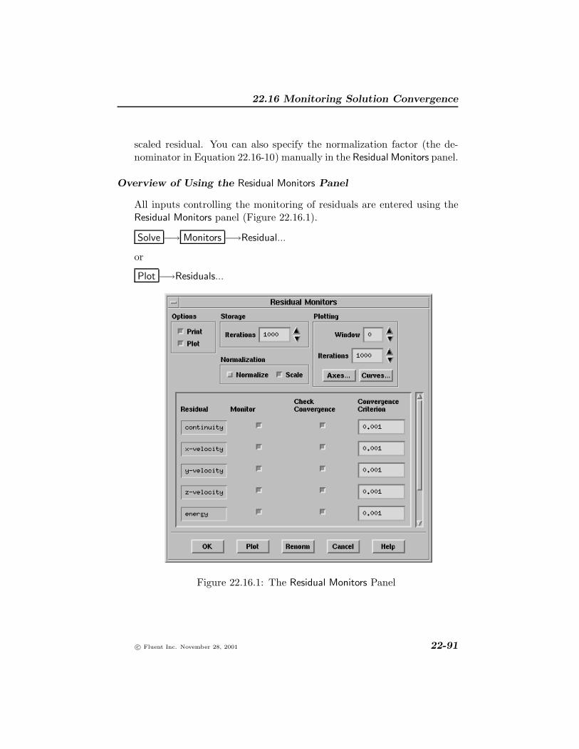
22.16 Monitoring Solution Convergence
scaled residual. You can also specify the normalization factor (the de-nominator in Equation 22.16-10) manually in the Residual Monitors panel.
Overview of Using the Residual Monitors Panel
All inputs controlling the monitoring of residuals are entered using theResidual Monitors panel (Figure 22.16.1).
Solve −→ Monitors −→Residual...
or
Plot −→Residuals...
Figure 22.16.1: The Residual Monitors Panel
c© Fluent Inc. November 28, 2001 22-91
Using the Solver
In general, you will only need to enable residual plotting and modify theconvergence criteria using this panel. Additional controls are availablefor disabling monitoring of particular residuals, and modifying normal-ization and plot parameters.
Printing and Plotting Residuals
By default, residual values for all relevant variables are printed in thetext (console) window after each iteration. If you wish to disable thisprintout, turn off Print under Options. To enable the plotting of residualsafter each iteration, turn on Plot under Options. Residuals will be plottedin the graphics window (with the window ID set in the Window field)during the calculation.
If you wish to display a plot of the current residual history, simply clickon the Plot push button.
Modifying Convergence Criteria
In addition to plotting and printing residual values during the calcula-tion, FLUENT will also check for convergence. If convergence is beingmonitored, the solution will stop automatically when each variable meetsits specified convergence criterion. Convergence checks can be performedonly for variables for which you are monitoring residuals (i.e., variablesfor which the Monitor option is enabled).
You can choose whether or not you want to check the convergence foreach variable by turning on or off the Check Convergence option for it inthe Residual Monitors panel. To modify the convergence criterion for aparticular variable, enter a new value in the corresponding ConvergenceCriterion field.
Plot Parameters
If you choose to plot the residual values (either interactively during thesolution or using the Plot button after calculations are complete), thereare several display parameters you can modify.
In the Window field under Plotting, you can specify the ID of the graphicswindow in which the plot will be drawn. When FLUENT is iterating, the
22-92 c© Fluent Inc. November 28, 2001

22.16 Monitoring Solution Convergence
active graphics window is temporarily set to this window to update theresidual plot, and then returned to its previous value. Thus, the residualplot can be maintained in a separate window that does not interfere withother graphical postprocessing.
By changing the Iterations entry under Plotting, you can modify the num-ber of residual history points to be displayed in the plot. If you specifyn points, FLUENT will display the last n history points. Since the yaxis is scaled by the minimum and maximum values of all points in theplot, you can “zoom in” on the end of the residual history by settingIterations to a value smaller than the number of iterations performed.If, for example, the residuals jumped early in the calculation when youturned on turbulence, that peak broadens the overall range in residualvalues, making the smaller fluctuations later on almost indistinguishable.By setting the value of Iterations so that the plot does not include thatearly peak, your y-axis range is better suited to the values that you areinterested in seeing.
You can also modify the attributes of the plot axes and the residualcurves. Click on the Axes... or Curves... button to open the Axes panelor Curves panel. See Sections 25.8.8 and 25.8.9 for details.
Disabling Monitoring
If your problem requires the solution of many equations (e.g., turbulencequantities and multiple species), a plot that includes all residuals maybe difficult to read. In such cases, you may choose to monitor only asubset of the residuals, perhaps those that affect convergence the most.You can indicate whether or not you want to monitor residuals for eachvariable by enabling or disabling the relevant check box in the Monitorlist of the Residual Monitors panel.
Controlling Normalization
By default, scaling of residuals (see Equations 22.16-4 and 22.16-9) isenabled and the default convergence criterion is 10−6 for energy and P-1equations and 10−3 for all other equations. Residual normalization (i.e.,dividing the residuals by the largest value during the first few iterations)is also available but disabled by default.
c© Fluent Inc. November 28, 2001 22-93

Using the Solver
Normalization can be used with both scaled and unscaled residuals. Notethat if normalization is enabled, the convergence criterion may need to beadjusted appropriately. See Section 22.19.1 for information about judg-ing convergence based on the different types of residual reports. (Boththe raw residuals and scaling factors are stored in the data file, so youcan switch between scaled and unscaled residuals.) To report unscaledresiduals, simply turn off the Scale option under Normalization.
If you switch from scaled to unscaled residuals (or vice versa) and you!are normalizing the residuals (as described below), you must click on theRenorm button to recompute the normalization factors.
If you wish to normalize the residuals (see Equation 22.16-7 or 22.16-10),turn on the Normalize option under Normalize. The Normalization Factorcolumn will be added to the panel at this time. FLUENT will normalizethe printed or plotted residual for each variable by the value indicatedas the Normalization Factor for that variable. The default NormalizationFactor is the maximum residual value after the first 5 iterations. To usethe maximum residual value after a different number of iterations (i.e.,specify a different value for M in Equation 22.16-7 or 22.16-10), you canmodify the Iterations entry under Normalization.
In some cases, the maximum residual may occur sometime after theiteration specified in the Iterations field. If this should occur, you can clickon the Renorm button to set the normalization factors for all variablesto the maximum values in the residual histories. Subsequent plots andprinted reports will use the new normalization factor.
You can also specify the normalization factor (the denominator in Equa-tion 22.16-7 or 22.16-10) explicitly. To modify the normalization factorfor a particular variable, enter a new value in the corresponding Normal-ization Factor field in the Residual Monitors panel.
If you wish to report unnormalized, unscaled residuals (Equation 22.16-3or 22.16-8), turn off the Normalize and Scale options under Normaliza-tion in the Residual Monitors panel. Note that unnormalized, unscaledresiduals are stored in the data file regardless of whether the reportedresiduals are normalized or scaled.
22-94 c© Fluent Inc. November 28, 2001
22.16 Monitoring Solution Convergence
Storing Residual History Points
Residual histories for each variable are automatically saved in the datafile, regardless of whether they are being monitored. You can controlthe number of history points to be stored by changing the Iterationsentry under Storage. By default, up to 1000 points will be stored. Ifmore than 1000 iterations are performed (i.e., the limit is reached), everyother point will be discarded—leaving 500 history points—and the next500 points will be stored. When the total hits 1000 again, every otherpoint will again be discarded, etc. If you are performing a large numberof iterations, you will lose a great deal of residual history informationabout the beginning of the calculation. In such cases, you should increasethe Iterations value to a more appropriate value. Of course, the largerthis number is, the more memory you will need, the longer the plottingwill take, and the more disk space you will need to store the data file.
Postprocessing Residual Values
If you are having solution convergence difficulties, it is often useful toplot the residual value fields (e.g., using contour plots) to determinewhere the high residual values are located. When you use one of thecoupled solvers, the residual values for all solution variables are availablein the Residuals... category in the postprocessing panels. (If you readcase and data files into FLUENT, you will need to perform at least oneiteration before the residual values are available for postprocessing.) Forthe segregated solver, however, only the mass imbalance in each cell isavailable by default.
If you want to plot residual value fields for a segregated solver calculation,you will need to do the following:
1. Read in the case and data files of interest (if they are not alreadyin the current session).
2. Use the expert command in the solve/set/ text menu to enablethe saving of residual values.
solve −→ set −→expert
c© Fluent Inc. November 28, 2001 22-95

Using the Solver
Among other questions, FLUENT will ask if you want to save cellresiduals for postprocessing. Enter yes or y, and keep the defaultsettings for all of the other questions (by pressing the <RETURN>key).
3. Perform at least one iteration.
The solution variables for which residual values are available will appearin the Residuals... category in the postprocessing panels. Note thatresidual values are not available for the radiative transport equationssolved by the discrete ordinates radiation model.
22.16.2 Monitoring Statistics
If you are solving a fully-developed periodic flow, you may want to mon-itor the pressure gradient or the bulk temperature ratio, as discussed inSection 8.3.
If you are solving an unsteady flow (especially if you are using the explicittime stepping option), you may want to monitor the “time” that haselapsed during the calculation. The physical time of the flow field startsat zero when you initialize the flow. (See Section 22.15 for details aboutmodeling unsteady flows.)
If you are using the adaptive time stepping method described in Sec-tion 22.15.2, you may want to monitor the size of the time step, ∆t.
You can use the Statistic Monitors panel (Figure 22.16.2) to print or plotthese quantities during the calculation.
Solve −→ Monitors −→Statistic...
The procedure for setting up this monitor is listed below:
1. Indicate the type of report you want by turning on the Print optionfor a printout or the Plot option for a plot. You can enable theseoptions simultaneously.
2. Select the appropriate quantity in the Statistics list.
22-96 c© Fluent Inc. November 28, 2001

22.16 Monitoring Solution Convergence
Figure 22.16.2: The Statistic Monitors Panel
3. If you are plotting the quantities, you can set any of the plottingoptions discussed below.
Plot Parameters
If you choose to plot the statistics, there are several display parametersyou can modify.
In the First Window field, you can specify the ID of the graphics windowin which the plot will be drawn (or in which the first plot will be drawn,if you are plotting more than one quantity.) When FLUENT is iterating,the active graphics window is temporarily set to this window to updatethe plot, and then returned to its previous value. Thus, the statisticsplot can be maintained in a separate window that does not interferewith other graphical postprocessing. Note that additional quantitiesthat you have selected in the Statistics list will be plotted in windowswith incrementally higher IDs.
You can also modify the attributes of the plot axes and curves. Click onthe Axes... or Curves... button to open the Axes panel or Curves panel.See Sections 25.8.8 and 25.8.9 for details.
c© Fluent Inc. November 28, 2001 22-97

Using the Solver
22.16.3 Monitoring Forces and Moments
At the end of each solver iteration, the lift, drag, and/or moment coeffi-cient can be computed and stored to create a convergence history. Youcan print and plot this convergence data, and also save it to an exter-nal file. The external file is written in the FLUENT XY plot file formatdescribed in Section 25.8.5. Monitoring forces can be useful when youare calculating external aerodynamics, for example, and you are espe-cially interested in the forces. Sometimes the forces converge before theresiduals have dropped three orders of magnitude, so you can save timeby stopping the calculation earlier than you would if you were moni-toring only residuals. (You should be sure to check the mass flow rateand heat transfer rate as well, using the Flux Reports panel describedin Section 26.2, to ensure that the mass and energy are being suitablyconserved.)
The force and moment coefficients use the reference values described in!Section 26.8. Specifically, the force coefficients use the reference area,density, and velocity, and the moment coefficients use the reference area,density, velocity and length.
Only the processed force coefficient data is saved. If you decide to change!any of the parameters controlling the force monitoring, such as the ref-erence values, force vector, moment center, moment axis, or wall zones,you may see a discontinuity in the data: the previous data is not up-dated. Usually, if you have made changes you will want to delete theprevious force coefficient data before continuing to iterate.
Monitoring Forces in Unsteady Flow Calculations
If you are calculating unsteady flow, the specified force reports will beupdated after each time step, rather than after each iteration. All otherfeatures of the force monitor and the related setup procedures are un-changed.
Overview of Using the Force Monitors Panel
You can use the Force Monitors panel (Figure 22.16.3) to print, plot, andsave the convergence history of the drag, lift, and moment coefficients
22-98 c© Fluent Inc. November 28, 2001
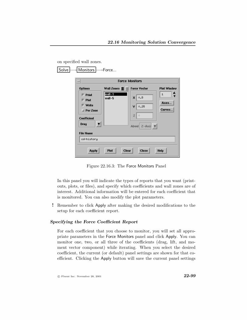
22.16 Monitoring Solution Convergence
on specified wall zones.
Solve −→ Monitors −→Force...
Figure 22.16.3: The Force Monitors Panel
In this panel you will indicate the types of reports that you want (print-outs, plots, or files), and specify which coefficients and wall zones are ofinterest. Additional information will be entered for each coefficient thatis monitored. You can also modify the plot parameters.
Remember to click Apply after making the desired modifications to the!setup for each coefficient report.
Specifying the Force Coefficient Report
For each coefficient that you choose to monitor, you will set all appro-priate parameters in the Force Monitors panel and click Apply. You canmonitor one, two, or all three of the coefficients (drag, lift, and mo-ment vector component) while iterating. When you select the desiredcoefficient, the current (or default) panel settings are shown for that co-efficient. Clicking the Apply button will save the current panel settings
c© Fluent Inc. November 28, 2001 22-99

Using the Solver
for the selected coefficient.
The procedure for specifying a force coefficient report is listed below:
1. Indicate the type of report you want (printout, plot, or file), asdescribed below.
2. If you want to monitor the force or moment on individual walls ina single printout, plot, or file, turn on the Per Zone option. Seebelow for details.
3. Choose the coefficient of interest by selecting Drag, Lift, or Momentin the Coefficient drop-down list.
4. In the Wall Zones list, select the wall zone(s) on which the selectedcoefficient is to be computed. If you are monitoring more thanone coefficient, the selected wall zones are often the same for eachcoefficient. If you want, however, you can have each coefficientcomputed on a different set of zones.
5. Depending on the coefficient selected, do one of the following:
• If you are monitoring the drag or lift coefficient, enter theX, Y, and Z components of the Force Vector along which theforces will be computed. The Force Vector heading will appearonly if you have selected Drag or Lift in the Coefficient drop-down list. By default, drag is computed in the x directionand lift in the y direction.
• If you are monitoring the moment coefficient, enter the Carte-sian coordinates (X, Y, and Z) of the Moment Center aboutwhich moments will be computed. The Moment Center head-ing will appear only if you have selected Moment in the Coef-ficient drop-down list. The default moment center is (0,0,0).You will also need to specify which component of the momentvector you wish to monitor. Presently, you can monitor onlyone component of the moment vector at a time. Select X-Axis, Y-Axis, or Z-Axis in the About drop-down list. (This listis active only if you have selected Moment in the Coefficientdrop-down list.) For two dimensional flows, only the momentvector about the z-coordinate axis exists.
22-100 c© Fluent Inc. November 28, 2001

22.16 Monitoring Solution Convergence
6. Click Apply and repeat the process for additional coefficients, ifdesired.
Printing, Plotting, and Saving Force Coefficient Histories
There are three methods available for reporting the selected force coef-ficients. To print the coefficient value(s) in the text (console) windowafter each iteration, turn on the Print option under Options in the ForceMonitors panel. To plot the coefficient in the graphics window indicatedin Plot Window, turn on the Plot option. If you want to save the valuesto a file, turn on the Write option and specify the File Name. You canenable any combination of these options simultaneously.
If you choose not to save the force coefficient data in a file, this informa-!tion will be lost when you exit the current FLUENT session.
If you wish to display a plot of the current force-coefficient history, simplyclick on the Plot button.
Plot Parameters
If you choose to plot the force coefficients (either interactively during thesolution or using the Plot button after calculations are complete), thereare several display parameters you can modify.
In the Plot Window field, you can specify the ID of the graphics windowin which the plot for each force coefficient will be drawn. When FLUENTis iterating, the active graphics window is temporarily set to this windowto update the plot, and then returned to its previous value. Thus, theforce-coefficient plots can be maintained in separate windows that do notinterfere with other graphical postprocessing.
You can also modify the attributes of the plot axes and the coefficientcurves. The same attributes apply to all force-monitor plots. Click onthe Axes... or Curves... button to open the Axes panel or Curves panel.See Sections 25.8.8 and 25.8.9 for details.
c© Fluent Inc. November 28, 2001 22-101

Using the Solver
Monitoring Forces and Moments on Individual Walls
By default, FLUENT will compute and monitor the total force or momentfor all of the selected walls combined together. If you have selectedmultiple walls and you want to monitor the force or moment on each wallseparately, you can turn on the Per Zone option in the Force Monitorspanel. The specified force vector or moment axis will apply to all selectedwalls.
If the monitor results are printed to the console (using the Print option),the force or moment on each wall will be printed in a separate column.If the results are plotted (using the Plot option), a separate curve foreach wall will be drawn in the specified plot window. If the resultsare written to a file (using the Write option), the file will be in a tab-separated column format based on the XY plot file format described inSection 25.8.5.
Discarding the Force-Monitoring Data
Should you decide that the data gathered by the force monitor are notuseful (e.g., if you are restarting the calculation or you changed one ofthe reference values), you can discard the accumulated data by clickingon the Clear button. The Clear button will delete all monitoring datafor the coefficient selected in the Coefficient drop-down list, includingthe associated history file (with the name in the File Name field). Whenyou use the Clear button, you will need to confirm the data discard ina Question dialog box. Only the force-monitoring data is removed usingthis operation; the solution data is not affected.
22-102 c© Fluent Inc. November 28, 2001
22.16 Monitoring Solution Convergence
22.16.4 Monitoring Surface Integrals
At the end of each solver iteration or time step, the average, mass av-erage, integral, flow rate, or other integral report of a field variable orfunction can be monitored on a surface. You can print and plot theseconvergence data, and also save them in an external file. The external fileis written in the FLUENT XY plot file format described in Section 25.8.5.The report types available are the same as those in the Surface Integralspanel, as described in Section 26.5.
Monitoring surface integrals can be used to check for both iteration con-vergence and grid independence. For example, you can monitor theaverage value of a certain variable on a surface. When this value stopschanging, you can stop iterating. You can then adapt the grid and re-converge the solution. The solution can be considered grid-independentwhen the average value on the surface stops changing between adaptions.
Overview of Defining Surface Monitors
You can use the Surface Monitors panel (Figure 22.16.4) to create sur-face monitors and indicate whether and when each one’s history is tobe printed, plotted, or saved. The Define Surface Monitor panel (Fig-ure 22.16.5), opened from the Surface Monitors panel, allows you to de-fine what each monitor tracks (i.e., the average, integral, flow rate, massaverage, or other integral report of a field variable or function on one ormore surfaces).
Defining Surface Monitors
You will begin the surface monitor definition procedure in the SurfaceMonitors panel (Figure 22.16.4).
Solve −→ Monitors −→Surface...
The procedure is as follows:
1. Increase the Surface Monitors value to the number of surface mon-itors you wish to specify. As this value is increased, additional
c© Fluent Inc. November 28, 2001 22-103
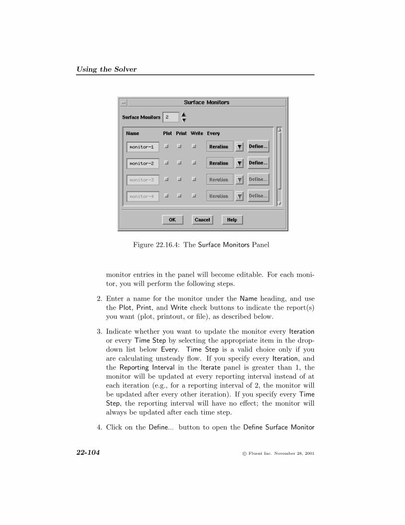
Using the Solver
Figure 22.16.4: The Surface Monitors Panel
monitor entries in the panel will become editable. For each moni-tor, you will perform the following steps.
2. Enter a name for the monitor under the Name heading, and usethe Plot, Print, and Write check buttons to indicate the report(s)you want (plot, printout, or file), as described below.
3. Indicate whether you want to update the monitor every Iterationor every Time Step by selecting the appropriate item in the drop-down list below Every. Time Step is a valid choice only if youare calculating unsteady flow. If you specify every Iteration, andthe Reporting Interval in the Iterate panel is greater than 1, themonitor will be updated at every reporting interval instead of ateach iteration (e.g., for a reporting interval of 2, the monitor willbe updated after every other iteration). If you specify every TimeStep, the reporting interval will have no effect; the monitor willalways be updated after each time step.
4. Click on the Define... button to open the Define Surface Monitor
22-104 c© Fluent Inc. November 28, 2001

22.16 Monitoring Solution Convergence
panel (Figure 22.16.5). Since this is a modal panel, the solver willnot allow you to do anything else until you perform steps 5–10,below.
Figure 22.16.5: The Define Surface Monitor Panel
5. In the Define Surface Monitor panel, choose the integration methodfor the surface monitor by selecting Integral, Area-Weighted Aver-age, Flow Rate, Mass Flow Rate, Mass-Weighted Average, Sum, FacetAverage, Facet Minimum, Facet Maximum, Vertex Average, VertexMinimum, or Vertex Maximum in the Report Type drop-down list.These methods are described in Section 26.5.
6. In the Surfaces list, choose the surface or surfaces on which youwish to integrate.
7. Specify the variable or function to be integrated in the Report Ofdrop-down list. First select the desired category in the upper drop-down list. You can then select one of the related quantities in the
c© Fluent Inc. November 28, 2001 22-105

Using the Solver
lower list. (See Chapter 27 for an explanation of the variables inthe list.)
8. If you are plotting the data or writing them to a file, specify theparameter to be used as the x-axis value (the y-axis value corre-sponds to the monitored data). In the X Axis drop-down list, selectIteration, Time Step, or Flow Time as the x-axis function againstwhich monitored data will be plotted or written. Time Step andFlow Time are valid choices only if you are calculating unsteadyflow. If you choose Time Step, the x axis of the plot will indicatethe time step, and if you choose Flow Time, it will indicate theelapsed time.
9. If you are plotting the monitored data, specify the ID of the graph-ics window in which the plot will be drawn in the Plot Windowfield. When FLUENT is iterating, the active graphics window istemporarily set to this window to update the plot, and then re-turned to its previous value. Thus, each surface-monitor plot canbe maintained in a separate window that does not interfere withother graphical postprocessing.
10. If you are writing the monitored data to a file, specify the FileName.
11. Remember to click OK in the Surface Monitors panel after you finishdefining all surface monitors.
Printing, Plotting, and Saving Surface Integration Histories
There are three methods available for reporting the selected surface in-tegration. To print the surface integration in the text (console) windowafter each iteration, turn on the Print option in the Surface Monitorspanel. To plot the integrated values in the graphics window indicatedin Plot Window (in the Define Surface Monitor panel), turn on the Plotoption in the Surface Monitors panel. If you want to save the values to afile, turn on the Write option in the Surface Monitors panel and specifythe File Name in the Define Surface Monitor panel. You can enable anycombination of these options simultaneously.
If you choose not to save the surface integration data in a file, this infor-!
22-106 c© Fluent Inc. November 28, 2001
22.16 Monitoring Solution Convergence
mation will be lost when you exit the current FLUENT session.
Plot Parameters
You can modify the attributes of the plot axes and curves used for eachsurface-monitor plot. Click on the Axes... or Curves... button in theDefine Surface Monitor panel for the appropriate monitor to open the Axespanel or Curves panel for that surface-monitor plot. See Sections 25.8.8and 25.8.9 for details.
22.16.5 Monitoring Volume Integrals
At the end of each solver iteration or time step, the volume or the sum,volume integral, volume average, mass integral, or mass average of afield variable or function can be monitored in one or more cell zones.You can print and plot these convergence data, and also save them inan external file. The external file is written in the FLUENT XY plot fileformat described in Section 25.8.5. The report types available are thesame as those in the Volume Integrals panel, as described in Section 26.6.
Monitoring volume integrals can be used to check for both iterationconvergence and grid independence. For example, you can monitor theaverage value of a certain variable in a particular cell zone. When thisvalue stops changing, you can stop iterating. You can then adapt thegrid and reconverge the solution. The solution can be considered grid-independent when the average value in the cell zone stops changing be-tween adaptions.
Overview of Defining Volume Monitors
You can use the Volume Monitors panel (Figure 22.16.6) to create vol-ume monitors and indicate whether and when each one’s history is tobe printed, plotted, or saved. The Define Volume Monitor panel (Fig-ure 22.16.7), opened from the Volume Monitors panel, allows you to de-fine what each monitor tracks (i.e., the volume or the sum, integral, oraverage of a field variable or function in one or more cell zones).
c© Fluent Inc. November 28, 2001 22-107

Using the Solver
Defining Volume Monitors
You will begin the volume monitor definition procedure in the VolumeMonitors panel (Figure 22.16.6).
Solve −→ Monitors −→Volume...
Figure 22.16.6: The Volume Monitors Panel
The procedure is as follows:
1. Increase the Volume Monitors value to the number of volume mon-itors you wish to specify. As this value is increased, additionalmonitor entries in the panel will become editable. For each moni-tor, you will perform the following steps.
2. Enter a name for the monitor under the Name heading, and usethe Plot, Print, and Write check buttons to indicate the report(s)you want (plot, printout, or file), as described below.
3. Indicate whether you want to update the monitor every Iterationor every Time Step by selecting the appropriate item in the drop-
22-108 c© Fluent Inc. November 28, 2001

22.16 Monitoring Solution Convergence
down list below Every. Time Step is a valid choice only if youare calculating unsteady flow. If you specify every Iteration, andthe Reporting Interval in the Iterate panel is greater than 1, themonitor will be updated at every reporting interval instead of ateach iteration (e.g., for a reporting interval of 2, the monitor willbe updated after every other iteration). If you specify every TimeStep, the reporting interval will have no effect; the monitor willalways be updated after each time step.
4. Click on the Define... button to open the Define Volume Monitorpanel (Figure 22.16.7). Since this is a modal panel, the solver willnot allow you to do anything else until you perform steps 5–10,below.
Figure 22.16.7: The Define Volume Monitor Panel
5. In the Define Volume Monitor panel, choose the integration methodfor the volume monitor by selecting Volume, Sum, Volume Integral,Volume-Average, Mass Integral, or Mass-Average in the Report Type
c© Fluent Inc. November 28, 2001 22-109

Using the Solver
drop-down list. These methods are described in Section 26.6.
6. In the Cell Zones list, choose the cell zone(s) on which you wish tointegrate.
7. Specify the variable or function to be integrated in the Report Ofdrop-down list. First select the desired category in the upper drop-down list. You can then select one of the related quantities in thelower list. (See Chapter 27 for an explanation of the variables inthe list.)
8. If you are plotting the data or writing them to a file, specify theparameter to be used as the x-axis value (the y-axis value corre-sponds to the monitored data). In the X Axis drop-down list, selectIteration, Time Step, or Flow Time as the x-axis function againstwhich monitored data will be plotted or written. Time Step andFlow Time are valid choices only if you are calculating unsteadyflow. If you choose Time Step, the x axis of the plot will indicatethe time step, and if you choose Flow Time, it will indicate theelapsed time.
9. If you are plotting the monitored data, specify the ID of the graph-ics window in which the plot will be drawn in the Plot Windowfield. When FLUENT is iterating, the active graphics window istemporarily set to this window to update the plot, and then re-turned to its previous value. Thus, each volume-monitor plot canbe maintained in a separate window that does not interfere withother graphical postprocessing.
10. If you are writing the monitored data to a file, specify the FileName.
11. Remember to click OK in the Volume Monitors panel after you finishdefining all volume monitors.
Printing, Plotting, and Saving Volume Integration Histories
There are three methods available for reporting the selected volume in-tegration. To print the volume integration in the text (console) window
22-110 c© Fluent Inc. November 28, 2001
22.17 Animating the Solution
after each iteration, turn on the Print option in the Volume Monitorspanel. To plot the integrated values in the graphics window indicatedin Plot Window (in the Define Volume Monitor panel), turn on the Plotoption in the Volume Monitors panel. If you want to save the values to afile, turn on the Write option in the Volume Monitors panel and specifythe File Name in the Define Volume Monitor panel. You can enable anycombination of these options simultaneously.
If you choose not to save the volume integration data in a file, this!information will be lost when you exit the current FLUENT session.
Plot Parameters
You can modify the attributes of the plot axes and curves used for eachvolume-monitor plot. Click on the Axes... or Curves... button in theDefine Volume Monitor panel for the appropriate monitor to open the Axespanel or Curves panel for that volume-monitor plot. See Sections 25.8.8and 25.8.9 for details.
22.17 Animating the Solution
During the calculation, you can have FLUENT create an animation ofcontours, vectors, XY plots, monitor plots (residual, statistic, force, sur-face, or volume), or the mesh (useful primarily for moving mesh simu-lations). Before you begin the calculation, you will specify and displaythe variables and types of plots you want to animate, and how often youwant plots to be saved. At the specified intervals, FLUENT will displaythe requested plots, and store each one. When the calculation is com-plete, you can play back the animation sequence, modify the view (forgrid, contour, and vector plots), if desired, and save the animation to aseries of hardcopy files or an MPEG file
Instructions for defining a solution animation sequence are provided inSection 22.17.1. Sections 22.17.2 and 22.17.3 describe how to play backand save the animation sequences you have created, and Section 22.17.4describes how to read a previously-saved animation sequence into FLU-ENT.
c© Fluent Inc. November 28, 2001 22-111

Using the Solver
22.17.1 Defining an Animation Sequence
You can use the Solution Animation panel (Figure 22.17.1) to create ananimation sequence and indicate how often each frame of the sequenceshould be created. The Animation Sequence panel (Figure 22.17.2),opened from the Solution Animation panel, allows you to define whateach sequence displays (e.g., contours or vectors of a particular variable),where it is displayed, and how each frame is stored.
You will begin the animation sequence definition in the Solution Anima-tion panel (Figure 22.17.1).
Solve −→ Animate −→Define...
Figure 22.17.1: The Solution Animation Panel
The procedure is as follows:
1. Increase the Animation Sequences value to the number of anima-tion sequences you wish to specify. As this value is increased,
22-112 c© Fluent Inc. November 28, 2001
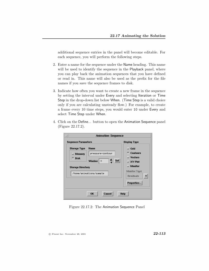
22.17 Animating the Solution
additional sequence entries in the panel will become editable. Foreach sequence, you will perform the following steps.
2. Enter a name for the sequence under the Name heading. This namewill be used to identify the sequence in the Playback panel, whereyou can play back the animation sequences that you have definedor read in. This name will also be used as the prefix for the filenames if you save the sequence frames to disk.
3. Indicate how often you want to create a new frame in the sequenceby setting the interval under Every and selecting Iteration or TimeStep in the drop-down list below When. (Time Step is a valid choiceonly if you are calculating unsteady flow.) For example, to createa frame every 10 time steps, you would enter 10 under Every andselect Time Step under When.
4. Click on the Define... button to open the Animation Sequence panel(Figure 22.17.2).
Figure 22.17.2: The Animation Sequence Panel
c© Fluent Inc. November 28, 2001 22-113

Using the Solver
5. Define the Sequence Parameters in the Animation Sequence panel.
(a) Specify whether you want FLUENT to save the animation se-quence frames in memory or on your computer’s hard driveby selecting Memory or Disk under Storage Type.
Note that a FLUENT metafile is created for each frame in the!animation sequence. These files contain information aboutthe entire scene, not just the view that is displayed in theplot. As a result, they can be quite large. By default, thefiles will be stored to disk. If you do not want to use up diskspace to store them, you can instead choose to store themin memory. Storing them in memory will, however, reducethe amount of memory available to the solver. Note that theplayback of a sequence stored in memory will be faster thanone stored to disk.
(b) If you selected Disk under Storage Type, specify the directorywhere you want to store the files in the Storage Directory field.(This can be a relative or absolute path.)
(c) Specify the ID of the graphics window where you want theplot to be displayed in the Window field, and click Set. (Thespecified window will open, if it is not already open.)
When FLUENT is iterating, the active graphics window is setto this window to update the plot. If you want to maintaineach animation in a separate window, specify a different Win-dow ID for each.
6. Define the display properties for the sequence.
(a) Under Display Type in the Animation Sequence panel, choosethe type of display you want to animate by selecting Grid,Contours, Vectors, XY Plot, or Monitor. If you choose Monitor,you can select any of the available types of monitor plots inthe Monitor Type drop-down list: Residuals, Force, Statistics,Surface, or Volume.
The first time that you select Contours, Vectors, or XY Plot, orone of the monitor types if you select Monitor, FLUENT willopen the corresponding panel (e.g., the Contours panel or the
22-114 c© Fluent Inc. November 28, 2001
22.17 Animating the Solution
Vectors panel) so you can modify the settings and generatethe display. To make subsequent modifications to the displaysettings for any of the display types, click the Properties...button to open the panel for the selected Display Type.
(b) Define the display in the panel for the selected Display Type(e.g., the Contours or Solution XY Plot panel), and click Displayor Plot.
You must click Display or Plot to initialize the scene to be!repeated during the calculation.
See below for guidelines on defining display properties for grid,contour, and vector displays.
7. Remember to click OK in the Solution Animation panel after youfinish defining all animation sequences.
Note that, when you click OK in the Animation Sequence panel for asequence, the Active button for that sequence in the Solution Animationpanel will be turned on automatically. You can choose to use a subsetof the sequences you have defined by turning off the Active button forthose that you currently do not wish to use.
Guidelines for Defining an Animation Sequence
If you are defining an animation sequence containing grid, contour, orvector displays, note the following when you are defining the display:
• If you want to include lighting effects in the animation frames,be sure to define the lights before you begin the calculation. SeeSection 25.2.6 for information about adding lights to the display.
• If you want to maintain a constant range of colors in a contouror vector display, you can specify a range explicitly by turningoff the Auto Range option in the Contours or Vectors panel. SeeSection 25.1.2 or 25.1.3 for details.
• Scene manipulations that are specified using the Scene Descriptionpanel will not be included in the animation sequence frames. View
c© Fluent Inc. November 28, 2001 22-115
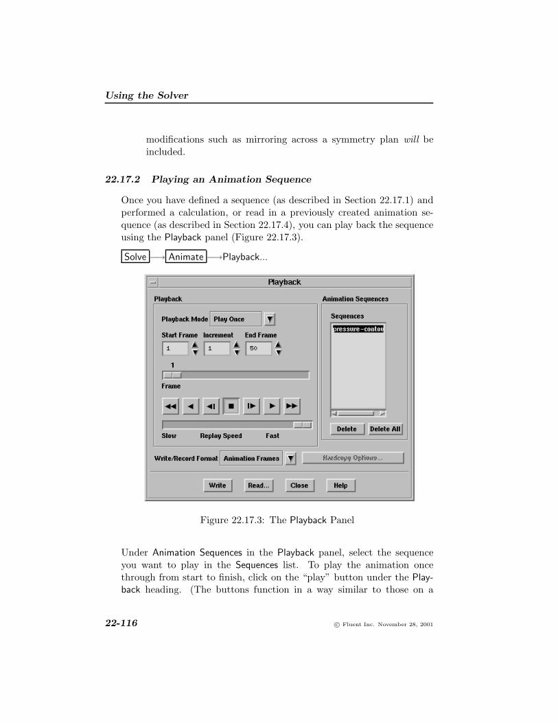
Using the Solver
modifications such as mirroring across a symmetry plan will beincluded.
22.17.2 Playing an Animation Sequence
Once you have defined a sequence (as described in Section 22.17.1) andperformed a calculation, or read in a previously created animation se-quence (as described in Section 22.17.4), you can play back the sequenceusing the Playback panel (Figure 22.17.3).
Solve −→ Animate −→Playback...
Figure 22.17.3: The Playback Panel
Under Animation Sequences in the Playback panel, select the sequenceyou want to play in the Sequences list. To play the animation oncethrough from start to finish, click on the “play” button under the Play-back heading. (The buttons function in a way similar to those on a
22-116 c© Fluent Inc. November 28, 2001

22.17 Animating the Solution
standard video cassette player. “Play” is the second button from theright—a single triangle pointing to the right.) To play the animationbackwards once, click on the “play reverse” button (the second from theleft—a single triangle point to the left). As the animation plays, theFrame scale shows the number of the frame that is currently displayed,as well as its relative position in the entire animation. If, instead of play-ing the complete animation sequence, you want to jump to a particularframe, move the Frame slider bar to the desired frame number, and theframe corresponding to the new frame number will be displayed in thegraphics window.
For smoother animations, turn on the Double Buffering option in the!Display Options panel (see Section 25.2.7). This will reduce screen flickerduring graphics updates.
Additional options for playing back animations are described below.
Modifying the View
If you want to replay the animation sequence with a different view of thescene, you can use your mouse to modify (e.g., translate, rotate, zoom)it in the graphics window where the animation is displayed. Note thatany changes you make to the view for an animation sequence will be lostwhen you select a new sequence (or reselect the current sequence) in theSequences list.
Modifying the Playback Speed
Different computers will play the animation sequence at different speeds,depending on the complexity of the scene and the type of hardware usedfor graphics. You may want to slow down the playback speed for optimalviewing. Move the Replay Speed slider bar to the left to reduce theplayback speed (and to the right to increase it).
Playing Back an Excerpt
You may sometimes want to play only one portion of a long animationsequence. To do this, you can modify the Start Frame and the End Frameunder the Playback heading. For example, if your animation contains 50
c© Fluent Inc. November 28, 2001 22-117
Using the Solver
frames, but you want to play only frames 20 to 35, you can set StartFrame to 20 and End Frame to 35. When you play the animation, it willstart at frame 20 and finish at frame 35.
“Fast-Forwarding” the Animation
You can “fast-forward” or “fast-reverse” the animation by skipping someof the frames during playback. To fast-forward the animation, you willneed to set the Increment and click on the fast-forward button (the lastbutton on the right—two triangles pointing to the right). If, for example,your Start Frame is 1, your End Frame is 15, and your Increment is 2, whenyou click on the fast-forward button, the animation will show frames 1,3, 5, 7, 9, 11, 13 and 15. Clicking on the fast-reverse button (the firstbutton on the left—two triangles pointing to the left) will show frames15, 13, 11,...1.
Continuous Animation
If you want the playback of the animation to repeat continuously, thereare two options available. To continuously play the animation from be-ginning to end (or from end to beginning, if you use one of the reverseplay buttons), select Auto Repeat in the Playback Mode drop-down list.To play the animation back and forth continuously, reversing the play-back direction each time, select Auto Reverse in the Playback Mode drop-down list.
To turn off the continuous playback, select Play Once in the PlaybackMode list. This is the default setting.
Stopping the Animation
To stop the animation during playback, click on the “stop” button (thesquare in the middle of the playback control buttons). If your animationcontains very complicated scenes, there may be a slight delay before theanimation stops.
22-118 c© Fluent Inc. November 28, 2001

22.17 Animating the Solution
Advancing the Animation Frame by Frame
To advance the animation manually frame by frame, use the third buttonfrom the right (a vertical bar with a triangle pointing to the right). Eachtime you click on this button, the next frame will be displayed in thegraphics window. To reverse the animation frame by frame, use thethird button from the left (a left-pointing triangle with a vertical bar).Frame-by-frame playback allows you to freeze the animation at pointsthat are of particular interest.
Deleting an Animation Sequence
If you want to remove one of the sequences that you have created or readin, select it in the Sequences list and click on the Delete button. If youwant to delete all sequences, click on the Delete All button.
Note that if you delete a sequence that has not yet been saved to disk (i.e.,!if you selected Memory under Storage Type in the Animation Sequencepanel), it will be removed from memory permanently. If you want tokeep any animation sequences that are stored only in memory, you shouldbe sure to save them (as described in Section 22.17.3) before you deletethem from the Sequences list or exit FLUENT.
22.17.3 Saving an Animation Sequence
Once you have created an animation sequence, you can save it in any ofthe following formats:
• Solution animation file containing the FLUENT metafiles
• Hardcopy files, each containing a frame of the animation sequence
• MPEG file containing each frame of the animation sequence
Note that, if you are saving hardcopy files or an MPEG file, you canmodify the view (e.g., translate, rotate, zoom) in the graphics windowwhere the animation is displayed, and save the modified view instead ofthe original view.
c© Fluent Inc. November 28, 2001 22-119

Using the Solver
Solution Animation File
If you selected Disk under Storage Type in the Animation Sequence panel,then FLUENT will save the solution animation file for you automati-cally. It will be saved in the specified Storage Directory, and its namewill be the Name you specified for the sequence, with a .cxa extension(e.g., pressure-contour.cxa). In addition to the .cxa file, FLUENTwill also save a metafile with a .hmf extension for each frame (e.g.,pressure-contour 2.hmf). The .cxa file contains a list of the associ-ated .hmf files, and tells FLUENT the order in which to display them.
If you selected Memory under Storage Type, then the solution animationfile (.cxa) and the associated metafiles (.hmf) will be lost when you exitfrom FLUENT, unless you save them as described below.
You can save the animation sequence to a file that can be read back intoFLUENT (see Section 22.17.4) when you want to replay the animation.As noted in Section 22.17.4, the solution animation file can be used forplayback in FLUENT independent of the case and data files that wereused to generate it.
To save a solution animation file (and the associated metafiles), selectAnimation Frames in the Write/Record Format drop-down list in the Play-back panel, and click on the Write button. FLUENT will save a .cxafile, as well as a .hmf file for each frame of the animation sequence.The filename for the .cxa file will be the specified sequence Name (e.g.,pressure-contour.cxa), and the filenames for the metafiles will con-sist of the specified sequence Name followed by a frame number (e.g.,pressure-contour 2.hmf). All of the files (.cxa and .hmf) will besaved in the current working directory.
Hardcopy File
You can also generate a hardcopy file for each frame in the animationsequence. This feature allows you to save your sequence frames to hard-copy files used by an external animation program such as ImageMagick.As noted above, you can modify the view in the graphics window beforeyou save the hardcopy files.
To save the animation as a series of hardcopy files, follow these steps:
22-120 c© Fluent Inc. November 28, 2001

22.17 Animating the Solution
1. Select Hardcopy Frames in the Write/Record Format drop-down listin the Playback panel.
2. If necessary, click on the Hardcopy Options... button to open theGraphics Hardcopy panel and set the appropriate parameters forsaving the hardcopy files. (If you are saving hardcopy files for usewith ImageMagick, for example, you may want to select the windowdump format. See Section 3.12.1 for details.) Click Apply in theGraphics Hardcopy panel to save your modified settings.
Do not click on the Save... button in the Graphics Hardcopy panel.!You will save the hardcopy files from the Playback panel in the nextstep.
3. In the Playback panel, click on the Write button. FLUENT willreplay the animation, saving each frame to a separate file. Thefilenames will consist of the specified sequence Name followed bya frame number (e.g., pressure-contour 2.ps), and they will allbe saved in the current working directory.
MPEG File
It is also possible to save all of the frames of the animation sequence inan MPEG file, which can be viewed using an MPEG decoder such asmpeg play. Saving the entire animation to an MPEG file will require lessdisk space than storing individual window dump files (using the hardcopymethod), but the MPEG file will yield lower-quality images.
As noted above, you can modify the view in the graphics window beforeyou save the MPEG file.
To save the animation to an MPEG file, follow these steps:
1. Select MPEG in the Write/Record Format drop-down list in thePlayback panel.
2. Click on the Write button.
FLUENT will replay the animation and save each frame to a sepa-rate scratch file, and then it will combine all the files into a single
c© Fluent Inc. November 28, 2001 22-121

Using the Solver
MPEG file. The name of the MPEG file will be the specified se-quence Name with a .mpg extension (e.g., pressure-contour.mpg),and it will be saved in the current working directory.
22.17.4 Reading an Animation Sequence
If you have saved an animation sequence to a solution animation file (asdescribed in Section 22.17.3), you can read that file back in at a latertime (or in a different session) and play the animation. Note that youcan read a solution animation file into any FLUENT session; you do notneed to read in the corresponding case and data files. In fact, you do notneed to read in any case and data files at all before you read a solutionanimation file into FLUENT.
To read a solution animation file, click on the Read... button in thePlayback panel. In the resulting Select File dialog box, specify the nameof the file to be read.
22.18 Executing Commands During the Calculation
As described in Sections 22.16 and 22.17, respectively, you can reportand monitor various quantities (e.g., residuals, force coefficients) and cre-ate animations of the solution while the solver is performing calculations.FLUENT also includes a feature that allows you to define your own com-mand(s) to be executed during the calculation at specified intervals. Forexample, you can ask FLUENT to export data to a third-party packagesuch as FIELDVIEW after every time step. You will specify a series oftext commands or use the GUI to define the steps to be performed.
If you want to save case or data files at intervals during the calcu-!lation, you must use the Autosave Case/Data panel (opened with theFile/Write/Autosave... menu item). See Section 3.3.4 for details.
22.18.1 Specifying the Commands to be Executed
You will indicate the command(s) that you want the solver to executeat specified intervals during the calculation using the Execute Commandspanel (Figure 22.18.1).
22-122 c© Fluent Inc. November 28, 2001

22.18 Executing Commands During the Calculation
Solve −→Execute Commands...
Figure 22.18.1: The Execute Commands Panel
The procedure is as follows:
1. Increase the Defined Commands value to the number of commandsyou wish to specify. As this value is increased, additional commandentries will become editable. For each command, you will performthe following steps.
2. Turn on the On check button next to the command if you wantit to be executed during the calculation. You may define multiplecommands and choose to use only a subset of them by turning offthe check button for those that you do not wish to use.
3. Enter a name for the command under the Name heading.
4. Indicate how often you want the command to be executed by set-ting the interval under Every and selecting Iteration or Time Step in
c© Fluent Inc. November 28, 2001 22-123

Using the Solver
the drop-down list below When. (Time Step is a valid choice onlyif you are calculating unsteady flow.) For example, to execute thecommand every 10 iterations, you would enter 10 under Every andselect Iteration under When.
If you specify an interval in iterations, be sure to keep the Reporting!Interval in the Iterate panel at its default value of 1.
5. Define the command by entering a series of text commands in theCommand field, or by entering the name of a command macro youhave defined (or will define) as described in Section 22.18.2.
If the command to be executed involves saving a file, see Sec-!tion 22.18.3 for important information.
22.18.2 Defining Macros
Macros that you define for automatic execution during the calculationcan also be used interactively by you during the problem setup or post-processing. For example, if you define a macro that performs a certaintype of adaption after each iteration, you can also use the macro toperform this adaption interactively.
Definition of a macro is accomplished as follows:
1. In the Execute Commands panel, click on the Define Macro... buttonto open the Define Macro panel (Figure 22.18.2). Since this is a“modal” panel, the solver will not allow you to do anything elseuntil you perform step 2, below.
2. In the Define Macro panel, specify a Name for the macro (e.g.,adapt1) and click on OK. (The Define Macro... button in the Exe-cute Commands panel will become the End Macro button.)
3. Perform the steps that you want the macro to perform. For exam-ple, if you want the macro to perform gradient adaption, open theGradient Adaption panel, specify the appropriate adaption functionand parameters, and click on Adapt to perform the adaption.
If the command to be executed involves saving a file, see Sec-!tion 22.18.3 for important information.
22-124 c© Fluent Inc. November 28, 2001
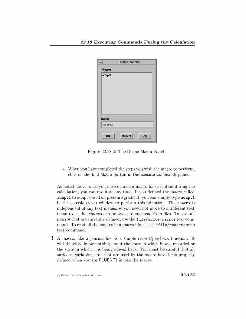
22.18 Executing Commands During the Calculation
Figure 22.18.2: The Define Macro Panel
4. When you have completed the steps you wish the macro to perform,click on the End Macro button in the Execute Commands panel.
As noted above, once you have defined a macro for execution during thecalculation, you can use it at any time. If you defined the macro calledadapt1 to adapt based on pressure gradient, you can simply type adapt1in the console (text) window to perform this adaption. This macro isindependent of any text menus, so you need not move to a different textmenu to use it. Macros can be saved to and read from files. To save allmacros that are currently defined, use the file/write-macros text com-mand. To read all the macros in a macro file, use the file/read-macrostext command.
A macro, like a journal file, is a simple record/playback function. It!will therefore know nothing about the state in which it was recorded orthe state in which it is being played back. You must be careful that allsurfaces, variables, etc. that are used by the macro have been properlydefined when you (or FLUENT) invoke the macro.
c© Fluent Inc. November 28, 2001 22-125

Using the Solver
22.18.3 Saving Files During the Calculation
If the command to be executed during the calculation involves saving afile, you must include a special character in the file name when you enterit in the Select File dialog box so that the solver will know to assign anew name to each file it saves. You can number the files by iterationnumber or by time step. (These special characters for numbering filesare also useful when you are saving window dumps for use in animations,as described in Section 3.12.1.) See Section 3.1.7 for details about thesespecial characters for filenames.
If you want to save case or data files at intervals during the calcu-!lation, you must use the Autosave Case/Data panel (opened with theFile/Write/Autosave... menu item). See Section 3.3.4 for details.
22.19 Convergence and Stability
Convergence can be hindered by a number of factors. Large numbersof computational cells, overly conservative under-relaxation factors, andcomplex flow physics are often the main causes. Sometimes it is difficultto know whether you have a converged solution. In the following sections,some of the numerical controls and modeling techniques that can beexercised to enhance convergence and maintain stability are examined.
• Section 22.19.1: Judging Convergence
• Section 22.19.2: Step-by-Step Solution Processes
• Section 22.19.3: Modifying Algebraic Multigrid Parameters
• Section 22.19.4: Modifying FAS Multigrid Parameters
• Section 22.19.5: Modifying Multi-Stage Time-Stepping Parameters
You should also refer to Sections 22.7 and 22.8 for information about howthe choice of discretization scheme or (for the segregated solver) pressure-velocity coupling scheme can affect convergence. Manipulation of under-relaxation parameters and multigrid settings to enhance convergence isdiscussed in Sections 22.9 and 22.19.3.
22-126 c© Fluent Inc. November 28, 2001

22.19 Convergence and Stability
22.19.1 Judging Convergence
There are no universal metrics for judging convergence. Residual defini-tions that are useful for one class of problem are sometimes misleadingfor other classes of problems. Therefore it is a good idea to judge con-vergence not only by examining residual levels, but also by monitoringrelevant integrated quantities such as drag or heat transfer coefficient.
For most problems, the default convergence criterion in FLUENT is suf-ficient. This criterion requires that the scaled residuals defined by Equa-tion 22.16-4 or 22.16-9 decrease to 10−3 for all equations except theenergy and P-1 equations, for which the criterion is 10−6.
Sometimes, however, this criterion may not be appropriate. Typicalsituations are listed below.
• If you make a good initial guess of the flow field, the initial conti-nuity residual may be very small leading to a large scaled residualfor the continuity equation. In such a situation it is useful to ex-amine the unscaled residual and compare it with an appropriatescale, such as the mass flow rate at the inlet.
• For some equations, such as for turbulence quantities, a poor ini-tial guess may result in high scale factors. In such cases, scaledresiduals will start low, increase as non-linear sources build up,and eventually decrease. It is therefore good practice to judge con-vergence not just from the value of the residual itself, but fromits behavior. You should ensure that the residual continues to de-crease (or remain low) for several iterations (say 50 or more) beforeconcluding that the solution has converged.
Another popular approach to judging convergence is to require that theunscaled residuals drop by three orders of magnitude. FLUENT providesresidual normalization for this purpose, as discussed in Sections 22.16.1and 22.16.1. In this approach the convergence criterion is that the nor-malized unscaled residuals should drop to 10−3. However, this require-ment may not be appropriate in many cases:
c© Fluent Inc. November 28, 2001 22-127
Using the Solver
• If you have provided a very good initial guess, the residuals maynot drop three orders of magnitude. In a nearly-isothermal flow, forexample, energy residuals may not drop three orders if the initialguess of temperature is very close to the final solution.
• If the governing equation contains non-linear source terms whichare zero at the beginning of the calculation and build up slowlyduring computation, the residuals may not drop three orders ofmagnitude. In the case of natural convection in an enclosure, forexample, initial momentum residuals may be very close to zerobecause the initial uniform temperature guess does not generatebuoyancy. In such a case, the initial nearly-zero residual is not agood scale for the residual.
• If the variable of interest is nearly zero everywhere, the residualsmay not drop three orders of magnitude. In fully-developed flow ina pipe, for example, the cross-sectional velocities are zero. If thesevelocities have been initialized to zero, initial (and final) residualsare both close to zero, and a three-order drop cannot be expected.
In such cases, it is wise to monitor integrated quantities, such as dragor overall heat transfer coefficient, before concluding that the solutionhas converged. It may also be useful to examine the un-normalizedunscaled residual, and determine if the residual is small compared tosome appropriate scale. Alternatively, the scaled residual defined byEquation 22.16-4 or 22.16-9 (the default) may be considered.
Conversely, it is possible that if the initial guess is very bad, the initialresiduals are so large that a three-order drop in residual does not guaran-tee convergence. This is specially true for k and ε equations where goodinitial guesses are difficult. Here again it is useful to examine overall in-tegrated quantities that you are particularly interested in. If the solutionis unconverged, you may drop the convergence tolerance, as described inSection 22.16.1.
22.19.2 Step-by-Step Solution Processes
One important technique for speeding convergence for complex problemsis to tackle the problem one step at a time. When modeling a problem
22-128 c© Fluent Inc. November 28, 2001

22.19 Convergence and Stability
with heat transfer, you can begin with the calculation of the isothermalflow. To solve turbulent flow, you might start with the calculation oflaminar flow. When modeling a reacting flow, you can begin by com-puting a partially converged solution to the non-reacting flow, possiblyincluding the species mixing. When modeling a discrete phase, such asfuel evaporating from droplets, it is a good idea to solve the gas-phaseflow field first. Such solutions generally serve as a good starting pointfor the calculation of the more complex problems. These step-by-steptechniques involve using the Solution Controls panel to turn equations onand off.
Selecting a Subset of the Solution Equations
FLUENT automatically solves each equation that is turned on using theModels family of panels. If you specify in the Viscous Model panel thatthe flow is turbulent, equations for conservation of turbulence quantitiesare turned on. If you specify in the Energy panel that FLUENT shouldenable energy, the energy equation is activated. Convergence can besped up by focusing the computational effort on the equations of primaryimportance. The Equations list in the Solution Controls panel allows youto turn individual equations on or off temporarily.
Solve −→ Controls −→Solution...
A typical example is the computation of a flow with heat transfer. Ini-tially, you will define the full problem scope, including the thermalboundary conditions and temperature-dependent flow properties. Fol-lowing the problem setup, you will use the Solution Controls panel totemporarily turn off the energy equation. You can then compute anisothermal flow field, remembering to set a reasonable initial value forthe temperature of the fluid.
This is possible only for the segregated solver; the coupled solvers solve!the energy equation together with the flow equations in a coupled man-ner, so you cannot turn off the energy equation as described above.
When the isothermal flow is reasonably well converged, you can turnthe energy equation back on. You can actually turn off the momentumand continuity equations while the initial energy field is being computed.
c© Fluent Inc. November 28, 2001 22-129
Using the Solver
When the energy field begins to converge well, you can turn the momen-tum and continuity equations back on so that the flow pattern can adjustto the new temperature field. The temperature will couple back into theflow solution by its impact on fluid properties such as density and vis-cosity. The temperature field will have no effect on the flow field if thefluid properties (e.g., density, viscosity) do not vary with temperature.In such cases, you can compute the energy field without turning the flowequations back on again.
If you have specified temperature-dependent flow properties, you should!be sure that a realistic value has been set for temperature throughoutthe domain before disabling calculation of the energy equation. If anunrealistic temperature value is used, the flow properties dependent ontemperature will also be unrealistic, and the flow field will be adverselyaffected. Instructions for initializing the temperature field or patching atemperature field onto an existing solution are provided in Section 22.13.
Turning Reactions On and Off
To solve a species mixing problem prior to solving a reacting flow, youshould set up the problem including all of the reaction information, andsave the complete case file. To turn off the reaction so that only thespecies mixing problem can be solved, you can use the Species Modelpanel to turn off the Volumetric Reactions.
Define −→ Models −→Species...
Once the species mixing problem has partially converged, you can returnto the Species Model panel and turn the Volumetric Reactions option onagain. You can then resume the calculation starting from the partiallyconverged data.
For combustion problems you may want to patch a hot temperature inthe vicinity of the anticipated reactions before you restart the calculation.See Section 22.13.2 for information about patching an initial value for aflow variable.
22-130 c© Fluent Inc. November 28, 2001

22.19 Convergence and Stability
22.19.3 Modifying Algebraic Multigrid Parameters
The default algebraic multigrid settings are appropriate for nearly allproblems, but in rare cases you may need to make minor adjustments.This section describes how to analyze the multigrid solver’s performanceto determine which parameters should be modified. It also provides ex-amples of suggested settings for particular types of problems and explainshow to set the multigrid parameters.
Analyzing the Algebraic Multigrid Solver
As mentioned earlier, in most cases the multigrid solver will not requireany special attention from you. If, however, you have convergence diffi-culties or you want to minimize the overall solution time by using moreaggressive settings, you can monitor the multigrid solver and modifythe parameters to improve its performance. (The instructions below as-sume that you have already begun calculations, since there is no need tomonitor the solver if you do not fit into one of the two categories above.)
To determine whether your convergence difficulties can be alleviated bymodifying the multigrid settings, you will check if the requested residualreduction is obtained on each grid level. To minimize solution time, youwill check to see if switching to a more powerful cycle will result in overallreduction of work by the solver.
Monitoring the Algebraic Multigrid Solver
The steps for monitoring the solver are as follows:
1. Set multigrid Verbosity to 1 or 2 in the Multigrid Controls panel.
Solve −→ Controls −→Multigrid...
2. Request a single iteration using the Iterate panel.
Solve −→Iterate...
If you set the verbosity to 2, the information printed in the console (text)window for each equation will include the following:
c© Fluent Inc. November 28, 2001 22-131

Using the Solver
• equation name
• equation tolerance (computed by the solver using a normalizationof the source vector)
• residual value after each fixed multigrid cycle or fine relaxation forthe flex cycle
• number of equations in each multigrid level, with the zeroth levelbeing the original (finest-level) system of equations
Note that the residual printed at cycle or relaxation 0 is the initial resid-ual before any multigrid cycles are performed.
When verbosity is set to 1, only the equation name, tolerance, and resid-uals are printed.
A portion of a sample printout is shown below:
pressure correction equation:tol. 1.2668e-05
0 2.5336e+001 4.9778e-012 2.5863e-013 1.9387e-01
multigrid levels:0 9181 4262 2053 974 455 216 107 4
Interpreting the Algebraic Multigrid Report
By default, the flex cycle is used for all equations except pressure correc-tion, which uses a V cycle. Typically, for a flex cycle only a few (5–10)
22-132 c© Fluent Inc. November 28, 2001

22.19 Convergence and Stability
relaxations will be performed at the finest level and no coarse levels willbe visited. In some cases one or two coarse levels may be visited. Ifthe maximum number of fine level relaxations is not sufficient, you maywant to increase the maximum number (as described in Section 22.19.3)or switch to a V cycle (as described in Section 22.19.3).
For pressure correction, a V cycle is used by default. If the maximumnumber of cycles (30 by default) is not sufficient, you can switch to a Wcycle (using the Multigrid Controls panel, as described in Section 22.19.3).Note that for the parallel solver, efficiency may deteriorate with a Wcycle. If you are using the parallel solver, you can try increasing themaximum number of cycles by increasing the value of Max Cycles in theMultigrid Controls panel under Fixed Cycle Parameters.
Solve −→ Controls −→Multigrid...
Changing the Maximum Number of Relaxations
To change the maximum number of relaxations, increase or decrease thevalue of Max Fine Relaxations or Max Coarse Relaxations in the MultigridControls panel (Figure 22.19.1) under Flexible Cycle Parameters.
Solve −→ Controls −→Multigrid...
Specifying the Multigrid Cycle Type
By default, the V cycle is used for the pressure equation and the flexcycle is used for all other equations. (See Section 22.5.2 for a descriptionof these cycles.) To change the cycle type for an equation, you will usethe top portion of the Multigrid Controls panel (Figure 22.19.1).
For each equation, you can choose Flexible, V-Cycle, W-Cycle, or F-Cyclein the adjacent drop-down list.
Setting the Termination and Residual Reduction Parameters
When you use the flex cycle for an equation, you can control the multigridperformance by modifying the Termination and/or Restriction criteria forthat equation at the top of the Multigrid Controls panel (Figure 22.19.1).
c© Fluent Inc. November 28, 2001 22-133

Using the Solver
Figure 22.19.1: The Multigrid Controls Panel
22-134 c© Fluent Inc. November 28, 2001

22.19 Convergence and Stability
Solve −→ Controls −→Multigrid...
The Restriction criterion is the residual reduction tolerance, β in Equa-tion 22.5-14. This parameter dictates when a coarser grid level must bevisited (due to insufficient improvement in the solution on the currentlevel). With a larger value of β, coarse levels will be visited less often(and vice versa). The Termination criterion, α in Equation 22.5-15, gov-erns when the solver should return to a finer grid level (i.e., when theresiduals have improved sufficiently on the current level).
For the V, W, or F cycle, the Termination criterion determines whetheror not another cycle should be performed on the finest (original) level. Ifthe current residual on the finest level does not satisfy Equation 22.5-15,and the maximum number of cycles has not been performed, FLUENTwill perform another multigrid cycle. (The Restriction parameter is notused by the V, W, and F cycles.)
Additional Algebraic Multigrid Parameters
There are several additional parameters that control the algebraic multi-grid solver, but there will usually be no need to modify them. Theseadditional parameters are all contained in the Multigrid Controls panel(Figure 22.19.1).
Solve −→ Controls −→Multigrid...
Coarsening Parameters
For all multigrid cycle types, you can control the maximum number ofcoarse levels (Max Coarse Levels under Coarsening Parameters) that willbe built by the multigrid solver. Sets of coarser simultaneous equationsare built until the maximum number of levels has been created, or thecoarsest level has only 3 equations. Each level has about half as manyunknowns as the previous level, so coarsening until there are only a fewcells left will require about as much total coarse-level coefficient storageas was required on the fine mesh. Reducing the maximum coarse levelswill reduce the memory requirements, but may require more iterationsto achieve a converged solution. Setting Max Coarse Levels to 0 turns offthe algebraic multigrid solver.
c© Fluent Inc. November 28, 2001 22-135

Using the Solver
Another coarsening parameter you can control is the increase in coarse-ness on successive levels. The Coarsen By parameter specifies the numberof fine grid cells that will be grouped together to create a coarse grid cell.The algorithm groups each cell with its closest neighbor, then groups thecell and its closest neighbor with the neighbor’s closest neighbor, con-tinuing until the desired coarsening is achieved. Typical values are inthe range from 2 to 10, with the default value of 2 giving the best per-formance, but also the greatest memory use. You should not adjustthis parameter unless you need to reduce the memory required to run aproblem.
Fixed Cycle Parameters
For the fixed (V, W, and F) multigrid cycles, you can control the numberof pre- and post-relaxations (β1 and β3 in Section 22.5.2). Pre Sweeps setsthe number of relaxations to perform before moving to a coarser level.Post Sweeps sets the number to be performed after coarser level correc-tions have been applied. Normally one post-relaxation is performed andno pre-relaxations are done (i.e., β3 = 1 and β1 = 0), but in rare cases,you may need to increase the value of β1 to 1 or 2.
Returning to the Default Multigrid Parameters
If you change the multigrid parameters, but you then want to returnto FLUENT’s default settings, you can click on the Default button inthe Multigrid Controls panel. FLUENT will change all settings to thedefaults, and the Default button will become the Reset button. To getyour settings back again, you can click on the Reset button.
22.19.4 Setting FAS Multigrid Parameters
For most calculations, you will not need to modify any FAS multigrid pa-rameters once you have set the number of coarse grid levels. If, however,you encounter convergence difficulties, you may consider the followingsuggested procedures.
Recall that FAS multigrid is used only by the coupled explicit solver.!
22-136 c© Fluent Inc. November 28, 2001

22.19 Convergence and Stability
Combating Convergence Trouble
Some problems may approach convergence steadily at first, but then theresiduals will level off and the solution will “get stuck.” In some cases(e.g., long thin ducts), this convergence trouble may be due to multigrid’sslow propagation of pressure information through the domain. In suchcases, you should turn off multigrid by setting Multigrid Levels to 0 inthe Solution Controls panel (under Solver Parameters).
Solve −→ Controls −→Solution...
“Industrial-Strength” FAS Multigrid
In some cases, you may find that your problem is converging, but atan extremely slow rate. Such problems can often benefit from a moreaggressive form of multigrid, which will speed up the propagation of thesolution corrections. For such problems, you can try the “industrial-strength” multigrid settings.
These settings are very aggressive and assume that the solution infor-!mation passed through the multigrid levels is somewhat accurate. Forthis reason, you should only attempt the procedure described here af-ter you have performed enough iterations that the solution is off to agood start. Using “industrial-strength” multigrid too early in the cal-culation process—when the solution is far from correct—will not helpconvergence and may cause the calculation to become unstable, as veryincorrect values are propagated quickly to the original grid. Note alsothat while these multigrid settings will usually reduce the total numberof iterations required to reach convergence, they will greatly increasethe computation time for each multigrid cycle. Thus the solver will beperforming fewer but longer iterations.
The strategy employed is as follows:
• Increase the number of iterations performed on each grid level be-fore proceeding to a coarser level
• Increase the number of iterations performed on each grid level afterreturning from a coarser level
c© Fluent Inc. November 28, 2001 22-137

Using the Solver
• Allow full correction transfer from one level to the next finer level,instead of transferring reduced values of the corrections
• Do not smooth the interpolated corrections when they are trans-ferred from a coarser grid to a finer grid
You can set all of the parameters for this strategy under FAS Multi-grid Controls in the Multigrid Controls panel (Figure 22.19.2) and thencontinue the calculation.
Solve −→ Controls −→Multigrid...
Increasing the number of iterations performed on each grid level beforeproceeding to a coarser level (the value of β1 described in Section 22.5.2)will improve the solution passed from each finer grid level to the nextcoarser grid level. Try increasing the value of Pre Sweeps (under FASMultigrid Controls, not under Algebraic Multigrid Controls) to 10.
Increasing the number of iterations performed on each level after return-ing from a coarser level will improve the corrections passed from eachcoarser grid level to the next finer grid level. Errors introduced on thecoarser grid levels can therefore be reduced before they are passed furtherup the grid hierarchy to the original grid. Try increasing the value ofPost Sweeps (under FAS Multigrid Controls, not under Algebraic MultigridControls) to 10.
By default, the full values of the multigrid corrections are not transferredfrom a coarser grid to a finer grid; only 60% of the value is transferred.This prevents large errors from transferring quickly up to the originalgrid and causing the calculation to become unstable. It also prevents a“good” solution from propagating quickly to the original grid, however.By increasing the Correction Reduction to 1, you can transfer the fullvalues from coarser to finer grid levels, speeding the propagation of thesolution and, usually, the convergence as well.
When the corrections on a coarse grid are passed back to the next finergrid level, the values are, by default, interpolated and then smoothed.Disabling the smoothing so that the actual value in a coarse grid cell isassigned to the fine grid cells that comprise it can also aid convergence.
22-138 c© Fluent Inc. November 28, 2001

22.19 Convergence and Stability
Figure 22.19.2: The Multigrid Controls Panel
c© Fluent Inc. November 28, 2001 22-139

Using the Solver
To turn off smoothing, set Correction Smoothing to 0. Large disconti-nuities between cells will be smoothed out implicitly as a result of theadditional Post Sweeps performed.
Additional Multigrid Parameters
There are several additional parameters that control the multigrid solver,but there will usually be no need to modify them. These additionalparameters are all contained in the Multigrid Controls panel.
Solve −→ Controls −→Multigrid...
Specifying the Multigrid Cycle Type
By default, the V cycle is used for the flow equations. (See Section 22.5.2for a description of the available cycles.) To change to a W cycle, youcan select it in the drop-down list next to Flow at the top of the MultigridControls panel (Figure 22.19.2).
Reducing the Time Step for Coarse Grid Levels
The Courant Number Reduction (at the bottom of the Multigrid Controlspanel) sets the factor by which to reduce the Courant number for coarsegrid levels (i.e., every level except the finest). Some reduction of timestep (such as the default 0.9) is typically required because the stabilitylimit cannot be determined as precisely on the irregularly shaped coarsergrid cells.
22.19.5 Modifying Multi-Stage Time-Stepping Parameters
The most common parameter you will change to control the multi-stagetime-stepping scheme is the Courant number. Instructions for modifyingthe Courant number are presented in Section 22.10, and procedures formodifying other less commonly changed parameters are provided in thissection.
22-140 c© Fluent Inc. November 28, 2001

22.19 Convergence and Stability
Using Residual Smoothing to Increase the Courant Number
Implicit residual smoothing (or averaging) is a technique that can beused to reduce the time step restriction of the solver, thereby allowing theCourant number to be increased. The implicit smoothing is implementedwith an iterative Jacobi method, as described in Section 22.4.3. You cancontrol residual smoothing in the Solution Controls panel.
Solve −→ Controls −→Solution...
By default, the number of Iterations for Residual Smoothing is set tozero, indicating that residual smoothing is disabled. If you increase theIterations counter to 1 or more, you can enter the Smoothing Factor. Asmoothing factor of 0.5 with 2 passes of the Jacobi smoother is usuallyadequate to allow the Courant number to be doubled.
Changing the Multi-Stage Scheme
It is possible to make several changes to the multi-stage time-steppingscheme itself. You can change the number of stages and set a new multi-stage coefficient for each stage. You can also control whether or notdissipation and viscous stresses are updated at each stage. These changesare made in the Multi-Stage Parameters panel (Figure 22.19.3).
Solve −→ Controls −→Multi-Stage...
You should not attempt to make changes to FLUENT’s multi-stage scheme!unless you are very familiar with multi-stage schemes and are interestedin trying a different scheme found in the literature.
Changing the Coefficients and Number of Stages
By default, the FLUENT multi-stage scheme uses 5 stages with coeffi-cients of 0.25, 0.166666, 0.375, 0.5, and 1.0 for the first through fifthstages, respectively. You can decrease the number of stages using thearrow buttons for Number of Stages in the Multi-Stage Parameters panel.(If you want to increase the number of stages, you will need to use thetext-interface command solve/set/multi-stage.) For each stage, youcan modify the Coefficient. Coefficients must be greater than 0 and lessthan 1. The final stage should always have a coefficient of 1.
c© Fluent Inc. November 28, 2001 22-141

Using the Solver
Figure 22.19.3: The Multi-Stage Parameters Panel
22-142 c© Fluent Inc. November 28, 2001

22.19 Convergence and Stability
Controlling Updates to Dissipation and Viscous Stresses
For each stage, you can indicate whether or not artificial dissipationand viscous stresses are evaluated. If a Dissipation box is selected for aparticular stage, artificial dissipation will be updated on that stage. Ifnot selected, artificial dissipation will remain “frozen” at the value ofthe previous stage. If a Viscous box is selected for a particular stage,viscous stresses will be updated on that stage. If not selected, viscousstresses will remain “frozen” at the value of the previous stage. Viscousstresses should always be computed on the first stage, and successiveevaluations will increase the “robustness” of the solution process, butwill also increase the expense (i.e., increase the CPU time per iteration).For steady problems, the final solution is independent of the stages onwhich viscous stresses are updated.
Resetting the Multi-Stage Parameters
If you change the multi-stage parameters, but you then want to return tothe default scheme set by FLUENT, you can click on the Default buttonin the Multi-Stage Parameters panel. FLUENT will change the values tothe defaults and the Default button will become the Reset button. Toget your values back again, you can click on the Reset button.
c© Fluent Inc. November 28, 2001 22-143

Using the Solver
22-144 c© Fluent Inc. November 28, 2001