Embed Size (px)
Citation preview

Chapter 22
Introduction to Probability Theory
Probability theory is a means of calculating the likelihood of different events occurring whenconducting some well-defined experiment.
Experiments: An experiment might be as simple as flipping a coin and observing whetherthe event heads or the event tails occurs. It might consist of buying a lottery ticketand observing how much money is gained or lost. It might also consist of executinga randomized algorithm on a given input instance and observing how long it executesand whether it gives the correct output.
Probability of an Event: The probability of event A is a real number p = Pr[A] ∈ [0, 1]that measures the fraction of times that the event occurs.
Definition: There are two ways of defining this probability: either by repeating theexperiment or by looking into how the experiment works. Either way, it involvescounting.
1) Running Many Times: If you repeat the experiment “independently” aninfinite number of times N , then the probability of an event p is defined tobe the fraction of those times in which the event occurs, that is, pN timesout of the N trials.
p = Pr[A] = limN→∞
The # of times event A occurs in N trials
N
2) Inner Workings: If we count all possible outcomes r of an experiment whereeach outcome is equally likely to occur, the probability p of event A can thenbe defined to be
p = Pr[A] =The # of r for which event A occurs
The # of r
Underlying Coin Flips: Suppose, for example, that the randomness forthe experiment comes from flipping a fair coin a fixed number of times.Then, r might be 〈heads, tails, heads, heads, . . . , tails〉.
1
Random Real in [0, 1]: Computers cannot actually flip coins. Instead, your pro-gram can call a system routine which tries to return some thing that is pseudorandom. A common routine rand returns a random real value x between zeroand one. You can use this to simulate other random distributions. For example,you can simulate a 6-sided die as follows. If x ∈ [0, 1
6) pretend that you rolled a
one. If x ∈ [16, 26), pretend you rolled a two and so on. This works because for any
0 ≤ a ≤ b ≤ 1, Pr [x ∈ [a, b]] = b− a.
Examples:
Coin Flip: Given this definition, it is easy to see that the probability of the eventheads when flipping a coin is p = 1
2.
Dying: To help get perspective on the probability p = 110,000,000
, it is approx-imately the probability of dying in the next five minutes, because peoplegenerally live at most 90 years which is 90 ·365 ·24 ·60/5 ≈ 10, 000, 000 blocksof 5 minutes and we approximate that you die in a random one of these.
Probability of x successes: Let Px denote the probability that there are ex-actly x successes when running n independent experiments each with successprobability p.
Px =
(n
x
)px(1−p)n−x =
n!
x! (n− x)!px(1−p)n−x.
This is because there are(nx
)ways of “choosing” x of the n experiments to be
the ones that will succeed. For each of these ways of choosing, the probabilitythat the x chosen experiments succeed is px and the probability that the n−xexperiments not chosen fail is (1−p)n−x.
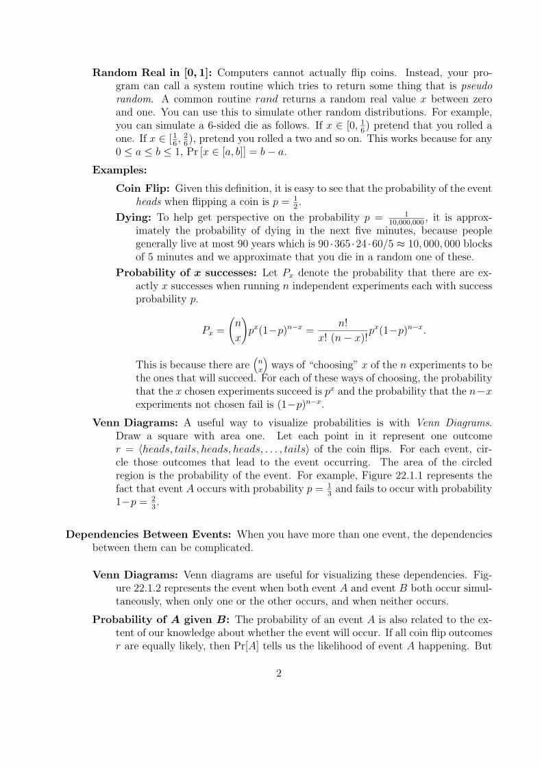
Venn Diagrams: A useful way to visualize probabilities is with Venn Diagrams.Draw a square with area one. Let each point in it represent one outcomer = 〈heads, tails, heads, heads, . . . , tails〉 of the coin flips. For each event, cir-cle those outcomes that lead to the event occurring. The area of the circledregion is the probability of the event. For example, Figure 22.1.1 represents thefact that event A occurs with probability p = 1
3and fails to occur with probability
1−p = 23.
Dependencies Between Events: When you have more than one event, the dependenciesbetween them can be complicated.
Venn Diagrams: Venn diagrams are useful for visualizing these dependencies. Fig-ure 22.1.2 represents the event when both event A and event B both occur simul-taneously, when only one or the other occurs, and when neither occurs.
Probability of A given B: The probability of an event A is also related to the ex-tent of our knowledge about whether the event will occur. If all coin flip outcomesr are equally likely, then Pr[A] tells us the likelihood of event A happening. But
2
AABA
A and BA and not B
B andnot A
not A and not B
V=3U=6
V=8U=4
V=1U=3
U=2V=5
A’
A’’
B
A
0 1/3 1
Figure 22.1: The four Venn diagrams. The first shows that the probability of event A isp = 1
3. The second shows the probability of events A and B happening simultaneously, the
probability of only one or the other occurring, and neither occurring. The third demonstratesevents A and B being independent, positively dependent, or negatively dependent. The lastshows a random variable V with Pr[V = 5] = 1
9.
suppose now, that we knew that event B happened. This narrows the possi-ble coin flip outcomes r to only those for which B occurs. See the B circle inFigure 22.1.2. Given this, the fraction of times that A will be happen is
Pr[A|B] =The # of r for which both A and B occur
The # of r for which event B occurs
=Pr[A and B]
Pr[B]
Independence and Dependence: Events can be dependent in different ways. Fig-ure 22.1.3 gives examples.
Definition of Independent Events: Events A and B are said to be indepen-dent if knowing that B occurs, does not give you any information aboutwhether A occurs. For example, when you flip two coins, their outcomes areindependent, that is, whether coin 1 is heads or tails does not affect whethercoin 2 is heads or tails. The formal definition is
Pr[A|B] = Pr[A].
An equivalent definition is that events A and B are independent if and onlyif
Pr[A and B] = Pr[A] · Pr[B].
See Exercises 22.0.1 and 22.0.2. Note that this second definition shows thesymmetry that if A is independent of B, then B is independent of A.I drew events A and B in Figure 22.1.3 to be independent events. If the areaof the box is one, of A is 1
25, and of B is 1
9, then area of the intersection A∩B
must be is 125
× 19. Given I eyeballed it, I make no promises. If the same two
circles were moved so they overlapped ever so slightly more, then the eventA and B would be positively dependent, while if they were moved to overlapever so slightly less, then they would be negatively dependent.
3
Positively Dependent: Events A′ and B are said to be positively dependentif they are more likely to occur together, that is Pr[A′|B] > Pr[A′] andPr[A′ and B] > Pr[A′] · Pr[B]. (Note that in Figure 22.1.3, Pr[A′|B] = 1.)Even if event A′ occurs if and only iff event B occurs, we do not really knowwhy this happens. This may occur because B “causes” A to happen, becauseA “causes” B to happen, or because some event C “causes” both A and B tohappen. A butterfly flapping its wings in Africa and a storm in Toronto arelikely independent events, but they say that in this interconnected chaoticworld, these events may be dependent.
Negatively Dependent: Events A′′ and B are said to be negatively dependentif they are less likely to occur together, that is Pr[A′′|B] < Pr[A′′] andPr[A′′ and B] > Pr[A′′] · Pr[B]. (Note that in Figure 22.1.3, Pr[A′′|B] = 0.)
Random Variables: Some experiments result in a value, like your winnings at gamblingor the running time of a randomized algorithm. The resulting value V is referred toas a random variable, as it takes on different values with different probabilities.
Examples:
Venn Diagram: In Figure 22.1.4, Pr[V = 5] = 19and Pr[V = 1] = 1
3.
Number of Heads: If you flip a coin n times, the number of times that youget a head is a random variable. If you flip it 4 times, V can take on valuesbetween 0 and 4. Pr[V = 2] = 3
8and Pr[V = 4] = 1
16
Indicator Variables: An indicator variable IA is a random variable which is 1when the event A being indicated occurs and zero when it does not.
Running Time: The running time T of a randomized algorithm is a randomvariable.
Expected Value: The expected value of a random variable is not the value that you expect,but is the average value if you were to repeat it many times.
Definition: The following are three equivalent definitions.
Average: Suppose again that the randomness comes from flipping a fair coin afixed number of times and let Vr denote the value of V when the outcomesof the coin flips is r. Each r is equally likely to occur. The expected value ofV is its average value.
Exp[V ] =
∑r Vr
The # of different r=∑
r
Pr[r]Vr
Value: Amore standard definition considers separately each value v that V mighttake on.
Exp[V ] =∑
values v
Pr[V = v] · v
4

Disjoint Events: Sometimes it is easier to partition the universe of possibleoutcomes into a set of events of your choosing. As in the “Average” definitionof expected value, an event could be that the coins came up as r. As in the“Value” definition of expected value, an event could be that random variableV takes on the value v. Or you can come up with your own set of events thatmake will make your calculations as easy as possible.
Exp[V ] =∑
disjoint events A
Pr[A] · [value of V during event A]
.
Examples:
Coin Flip: If you get V = 1 for a head and V = −1 for a tail, then the expectedamount is Exp[V ] = 1
2· 1 + 1
2· (−1) = 0.
Venn Diagram: In Figure 22.1.4, the expected value of V is Exp[V ] =∑v Pr[V = v] · v = 1
9· 5 + 1
3· 1 + 2
9· 8 + 1
3· 3 = 32
3.
Lotteries: If you pay $5 for a lottery ticket and with probability p = 110,000,000
you win $25,000,000, then your expected winnings are (1 − 110,000,000
) · 0 +1
10,000,000· 25, 000, 000 = $2.50. But you paid $5. Hence, you expect to lose
half your money. This is surprising, because I expect you will lose all of yourmoney.
Expected Happiness: Money is not everything though. What is your expectedgain in happiness? I claim having $5 given your current level of wealth addsmore to your happiness than having $5 when you already have $25,000,000.This proves that happiness does not increase linearly with money. In fact, Iwould guess it is more logarithmic because no matter how much you have,if the amount you have doubles, your happiness increases by more or less afixed amount. So let’s guess that buying a roti with your $5 would bringyou one unit of happiness and winning $25,000,000 would bring you 1,000units of happiness. You say more? Okay, 100,000 units. Then your expectedhappiness gained by buying a ticket is (1− 1
10,000,000)·(−1)+ 1
10,000,000·100, 000 ≈
(−1) + 0.001 ≈ −1, i.e. you lose.
Expected Number: If you flip a coin n times, the expected number of timesthat you get a head is n
2.
Indicator Variables: The expected value of an indicator variable IA equals theprobability of the event A, that is Exp[IA] = Pr[A] · 1+Pr[not A] · 0 = Pr[A].
Linearity of Sum of Expectation: A very useful fact is that the expectation of thesum is equal to the sum of the expectations. Let V1, V2, V3, . . . , Vn be n randomvariables, which may or may not be dependent in complicated ways. If you forma new random variable denoted V ′ whose value on every outcome of the coins isthe sum of the Vi, then
Exp [V ′] = Exp
[∑
i
Vi
]=∑
i
Exp [Vi] .
5

Venn Diagram: In Figure 22.1.4,Exp[V ] =
∑v Pr[V = v] · v = 1
9· 5 + 1
3· 1 + 2
9· 8 + 1
3· 3 = 32
3.
Exp[U ] =∑
u Pr[U = u] · u = 19· 2 + 1
3· 3 + 2
9· 4 + 1
3· 6 = 41
9.
Exp[(V + U)] =∑
w Pr[(V + U) = w] · w = 19· 7 + 1
3· 4 + 2
9· 12 + 1
3· 9 = 77
9.
We can check that Exp[(V + U)] = 779= 32
3+ 41
9= Exp[V ] + Exp[U ].
Proof: The proof that the expectation of the sum is equal to the sum ofthe expectations is as follows. The formal definition of the expectation isExp [U+V ] =
∑w Pr [U+V = w] ·w, however, it is not clear what to do with
this. It is better to break the universe of possibilities into finer events. Forevery tuple 〈u, v〉, consider the event that U = u and V = v. Note that whenthis event occurs, we know that the random variable [U+V ] takes on thevalue u+ v. This gives that
Exp[U+V ] =∑
disjoint events A
Pr[A] · [value of [U+V ] during event A]
=∑
〈u,v〉
Pr [U = u and V = v] · (u+ v)
The distributive and the commutative laws gives that [p · (u+ v)] + [p′ · (u′ +v′)] = [pu+pv]+ [p′u′+p′v′] = [pu+p′u′]+ [pv+p′v′]. Such rearranging gives
Exp[U+V ] =
∑
〈u,v〉
Pr [U = u and V = v] · u+
∑
〈u,v〉
Pr [U = u and V = v] · v
Think of a matrix of values indexed by u and v. The sum of the entries canbe obtained by summing them up. It can also be obtained by summing eachrow and then summing these sums or by summing each column and thensumming these sums.
Exp[U+V ] =∑
u
[∑
v
Pr [U = u and V = v] · u]+
∑
v
[∑
u
Pr [U = u and V = v] · v]
We now use the reverse of the distributive law, pu+ p′u = (p+ p′)u.
Exp[U+V ] =∑
u
[∑
v
Pr [U = u and V = v]
]· u+
∑
v
[∑
u
Pr [U = u and V = v] · v]
6
Fix some value u. What is∑
v Pr [U = u and V = v]? If you think of theVenn diagram, Pr [U = u] is the area of the union of all the areas in whichU = u. In some of those areas, V = v and in some of them V = v′. It followsthat
∑v Pr [U = u and V = v] = Pr [U = u]. Hence,
Exp[U+V ] =∑
u
Pr [U = u] · u+∑
v
Pr [V = v] · v
but by the definition of expected values this gives
Exp[U+V ] = Exp [U ] + Exp [V ]
Expected Number of Successes: If you have n trials where each trial has suc-cess with probability p, the expected number of successes is pn. This is trueeven if the success of each trial dependent in complicated ways on each other.
Proof: A simple proof is as follows.
Exp [Numb of successes] = Exp
[∑
i
Ii
]=∑
i
Exp [Ii]
=∑
i
[p · 1 + (1−p) · 0] = pn
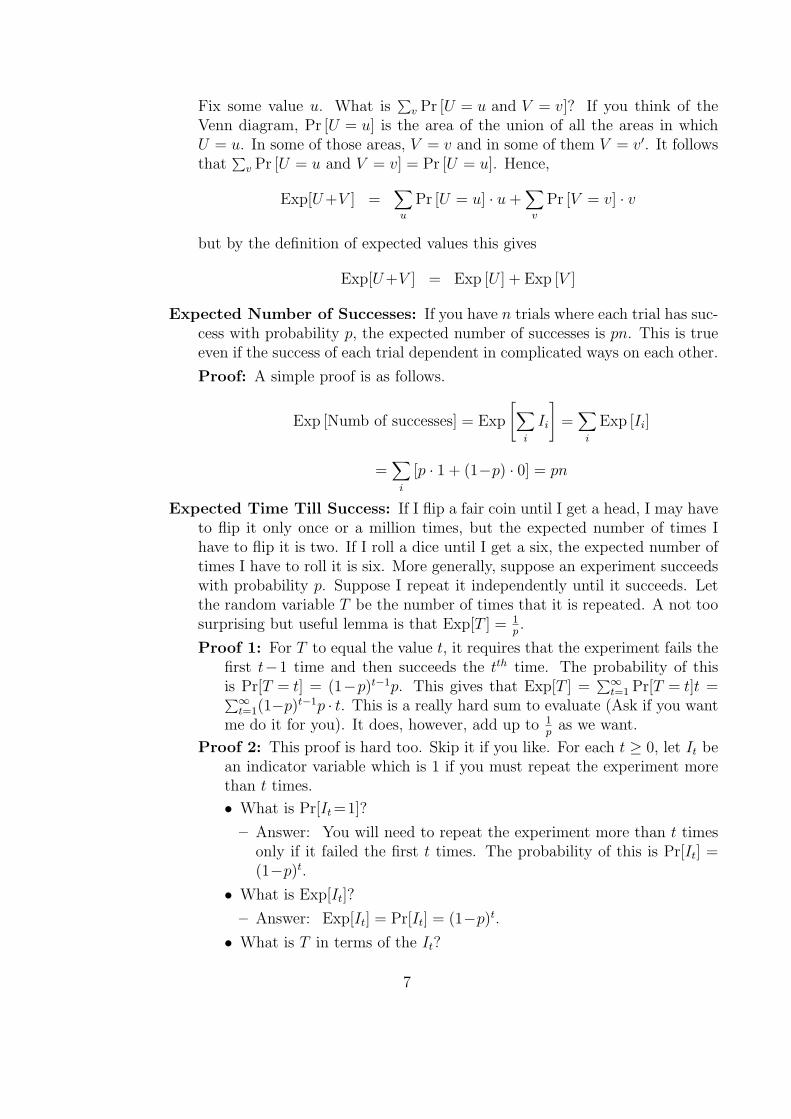
Expected Time Till Success: If I flip a fair coin until I get a head, I may haveto flip it only once or a million times, but the expected number of times Ihave to flip it is two. If I roll a dice until I get a six, the expected number oftimes I have to roll it is six. More generally, suppose an experiment succeedswith probability p. Suppose I repeat it independently until it succeeds. Letthe random variable T be the number of times that it is repeated. A not toosurprising but useful lemma is that Exp[T ] = 1
p.
Proof 1: For T to equal the value t, it requires that the experiment fails thefirst t−1 time and then succeeds the tth time. The probability of thisis Pr[T = t] = (1−p)t−1p. This gives that Exp[T ] =
∑∞t=1 Pr[T = t]t =∑∞
t=1(1−p)t−1p · t. This is a really hard sum to evaluate (Ask if you wantme do it for you). It does, however, add up to 1
pas we want.
Proof 2: This proof is hard too. Skip it if you like. For each t ≥ 0, let It bean indicator variable which is 1 if you must repeat the experiment morethan t times.
• What is Pr[It=1]?
– Answer: You will need to repeat the experiment more than t timesonly if it failed the first t times. The probability of this is Pr[It] =(1−p)t.
• What is Exp[It]?
– Answer: Exp[It] = Pr[It] = (1−p)t.
• What is T in terms of the It?
7

– Answer: T =∑
t≥0 It is the total number of experiments tried.
• What is Exp[T ]? Hint: For 0 ≤ q < 1,∑
t≥0 qt = 1
1−q.
– Answer: Exp[T ] = Exp[∑
t≥0 It] =∑
t≥0 Exp[It] =∑
t≥0(1−p)t = 1p.
Expectation of Product: The same thing is true for the product of random variableif the random variables are independent and is not necessarily true if they aredependent.
Proof when Independent: We prove as follows that if V1, V2, V3, . . . , Vn areindependent random variables, then
Exp [V ′] = Exp [ΠiVi] = ΠiExp [Vi] .
The proof begins the way it did for the sum of expectations.
Exp[U×V ] =∑
w
Pr [U × V = w] · w =∑
u
∑
v
Pr [U = u and V = v] · (u× v)
Because the events are independent we have that Pr [U = u and V = v] =Pr [U = u] × Pr [V = v]. Then commutativity gives (p × p′) · (u × v) = (p ·u)× (p′ · v).
Exp[U×V ] =∑
u
∑
v
[Pr [U = u] · u]× [Pr [V = v] · v]
We now use the distributed law that pq+ pq′ + p′q+ p′q′ = (p+ p′)× (q+ q′).
Exp[U×V ] =
[∑
u
Pr [U = u] · u]×[∑
v
Pr [V = v] · v]= Exp [U ]× Exp [V ]
Proof when Not Independent: We prove as follows that if the random vari-ables are dependent than the previous result is not necessarily true.Suppose that V1 = V2 = 0 with probability 1
2and V1 = V2 = 2 with probability
12. Then Exp[V1] = Exp[V2] =
12·0+ 1
2·2 = 1. Exp[V1·V2] =
12·(0·0)+ 1
2·(2·2) =
2. This is different than Exp[V1] · Exp[V2].
Random Walks: Consider a line (side walk with squares) with a wall at i = 0 and a wallat i = n.
Completely Drunk: Each time step, the drunk man is standing at some square i andwith probability 1
2stumbles one square forward and with probability 1
2stumbles
one square backwards. When i = 0, he only goes forward. What is the expectednumber of time steps starting at i = 0 until the man to first gets to i = n. Guess.Is it 2n, n2, 2n or something else?
Proof: Let ti denote the expected number of time steps starting at square i untilthe man to first gets to square i+1. We can write a recurrence relation. Withprobability 1
2, he goes forward and it takes him only one step. However, with
probability 12, he goes backwards and that one step takes him to square i− 1.
8
From here, the expected number of time steps until he first returns to squarei is ti−1. From here, the expected number of time steps until he first getsto square i+1 is ti. Because the expectation of the sum is the sum of theexpectations, we get the following
ti =12[1] + 1
2[1 + ti−1 + ti]
12ti = 1 + 1
2ti−1
ti = 2 + ti−1 = 2 + 2 + ti−2 = 2j + ti−j = 2i+ t0 = 2i+ 1
.The expected number of time steps starting at i = 0 until the man to firstgets to i = n is the expected number of time steps until he first gets to i = 1plus the the expected number until he first gets from there to i = 2 and soon, which is
n−1∑
i=0
ti =n−1∑
i=0
2i+ 1 = n2 +Θ(1).
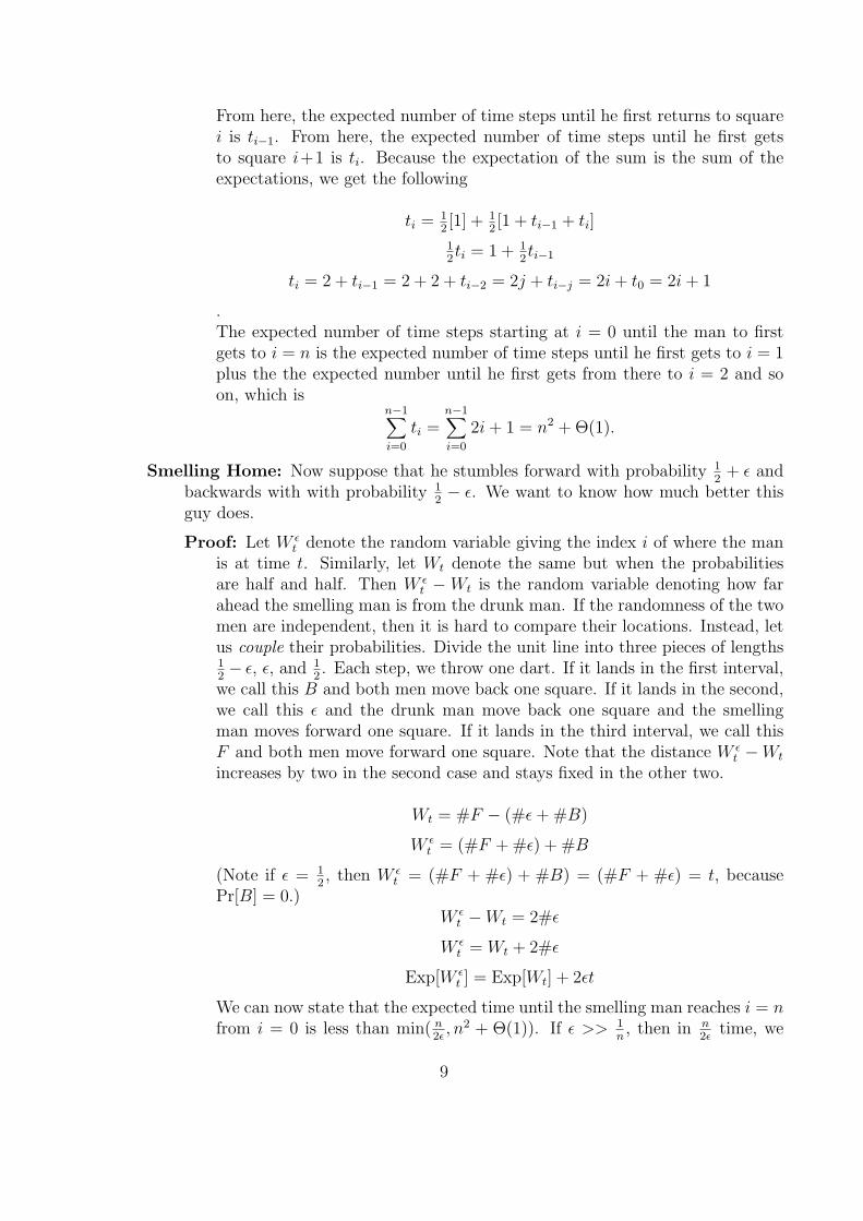
Smelling Home: Now suppose that he stumbles forward with probability 12+ ǫ and
backwards with with probability 12− ǫ. We want to know how much better this
guy does.
Proof: Let W ǫt denote the random variable giving the index i of where the man
is at time t. Similarly, let Wt denote the same but when the probabilitiesare half and half. Then W ǫ
t − Wt is the random variable denoting how farahead the smelling man is from the drunk man. If the randomness of the twomen are independent, then it is hard to compare their locations. Instead, letus couple their probabilities. Divide the unit line into three pieces of lengths12− ǫ, ǫ, and 1
2. Each step, we throw one dart. If it lands in the first interval,
we call this B and both men move back one square. If it lands in the second,we call this ǫ and the drunk man move back one square and the smellingman moves forward one square. If it lands in the third interval, we call thisF and both men move forward one square. Note that the distance W ǫ
t −Wt
increases by two in the second case and stays fixed in the other two.
Wt = #F − (#ǫ+#B)
W ǫt = (#F +#ǫ) + #B
(Note if ǫ = 12, then W ǫ
t = (#F + #ǫ) + #B) = (#F + #ǫ) = t, becausePr[B] = 0.)
W ǫt −Wt = 2#ǫ
W ǫt = Wt + 2#ǫ
Exp[W ǫt ] = Exp[Wt] + 2ǫt
We can now state that the expected time until the smelling man reaches i = nfrom i = 0 is less than min( n
2ǫ, n2 + Θ(1)). If ǫ >> 1
n, then in n
2ǫtime, we
9

can’t expect the drunk man to have gotten very far, but we can expect thesmelling man to be n steps in front of the him and hence past the i = n line.On the other hand, if ǫ << 1
n, then in n2 + Θ(1)) time, we can’t expect the
smelling man to have gotten very far ahead of the drunk man, but we canexpect the drunk man to have reached the i = n line and so so will have thesmelling man.
Plotting Probability: Other useful ways to visualize random variables are using the fol-lowing three functions.
Value from Point: A Venn graph like Figure 22.1.4 labels each point in the unitsquare with a real number. You can imagine throwing a dart at the unit squareuniformly at random (meaning each point in the square is equally likely to gethit. The value of the random variable V will be the real value labeling the unitsquare at that point. Using the unit square has the advantage that you can dawnit nicely as done in Figure 22.1.4. However, instead of a unit square, you couldjust as easily use the unit line. We will use function V̂ : [0, 1] ⇒ R to label eachreal value point x in the unit interval [0, 1] with a real number. You can imaginethrowing a dart at the unit interval uniformly at randomly obtaining some realvalue x. The value of the random variable V will be the real value V̂ (x) labelingthe unit interval at that point x. In general, V̂ can be an arbitrary function, butfor are purposes here, we might as well assume that the values V are sorted sothat V̂ (x) is a non-decreasing function.
Figure 22.1.4: For example, the random variable V in Figure 22.1.4. has V̂ (x) =1 for x ∈ [0, 1
3], V̂ (x) = 3 for x ∈ [1
3, 23], V̂ (x) = 5 for x ∈ [2
3, 79], and finally
V̂ (x) = 8 for x ∈ [79, 1].
Real in [0,6 :] As as second example, let V̂ (x) = 6x and then V is a randomvariable that uniformly takes on a random real value from 0 to 6. Note, thatbecause V can take on any real from 0 to 6, the probability it takes on anyparticular value like 2 is effectively zero. On the other hand, Pr[V ≤ v] is26= 1
3.
Pr[V ≤ v]: The second function P(≤) : R ⇒ [0, 1] used to describe a random variableV is defined to be
P(≤)(v) = Pr[V ≤ v].
Increasing: Note that P(≤)(−∞) = Pr[V ≤ −∞] = 0. Then P(≤)(v) increaseswith v until P(≤)(∞) = Pr[V ≤ ∞] = 1.
Figure 22.1.4: For example, the random variable V in Figure 22.1.4. hasP(≤)(v) = 0 for v ∈ [0, 1), P(≤)(v) =
13for v ∈ [1, 3), P(≤)(v) =
23for v ∈ [3, 5),
P(≤)(v) =79for v ∈ [5, 8), and P(≤)(v) = 1 for v ∈ [8,∞).
Real in [0,6 :] When V is a random variable that uniformly takes on a randomreal value from 0 to 6, then for v ∈ [0, 6], P(≤)(v) = Pr[V ≤ v] = v
6.
P(≤) Inverse of V̂ : Suppose that the previously mentioned function V̂ is strictly
increasing. Hence, if V̂ (x) = v, then V̂ (x′) ≤ v for all x′ ∈ [0, x] and V̂ (x′) > v
10

for all x′ ∈ (x, 1]. This gives that P(≤)(v) = Pr[V ≤ v] = x and hence that
P(≤)(V̂ (x)) = x, i.e. V̂ and P(≤) are inverses of each other. If V̂ is nondecreasing, but could take on the same value for a while, then it is a littletrickier, but one can show that V̂ (P(≤)(v)) = v.
Pr[V = v]: The third function P= used to describe a random variable V is defined toexpress Pr[V = v].
Discrete V : If the random variable V takes on discrete values v1, v2, . . . , vr,then a histogram has a place in the X axis for each of the possible val-ues v1, v2, . . . , vr, and above vi is a bar of width one and height (and area)Pr[V = vi]. Denote the resulting curve by P(=). Note that the “area” ofunder this curve is one because
∑i Pr[V = vi] must be one.
Figure 22.1.4: For example, the random variable V in Figure 22.1.4. hasP=(1) =
13, P=(3) =
13, P=(5) =
19, and P=(8) =
29.
Continuous V : If the random variable V takes a range of real values, then doinga histogram is more complicated because then Pr[V = v] is effectively zero.
Infinitesimals: What we will do instead is break the range of values v intointervals each of width δv, where δv is your favorite some infinitesimalvalue. Then instead of considering Pr[V = v], we consider Pr[V ∈ [v, v+δv]]. Though this probability is still an infinitesimal, we can still imaginethis being bigger than zero.
Histogram: We will now build a histogram, just as we did in the discretecase. It has a place in the X axis for each of the v intervals. Above v is abar of width δv, area Pr[V ∈ [v, v+δv]], and height Pr[V ∈[v,v+δv]]
δv. Denote
the resulting curve by P(=).
Real in [0,6 :] When V is a random variable that informally takes on a
random real value from 0 to 6, then P(=)(v) = Pr[V ∈[v,v+δv]]δv
= δv/6δv
=16. This curve is constant (P(=)(v) = 1
6), which is the case for uniform
distributions.
Pr[V ∈ [v1, v2]]: From this curve we can read off any probability, because
Pr[V ∈ [v1, v2]] =∑
intervals v∈[v1,v2]
Pr[V ∈ [v, v+δv]
=∑
intervals v∈[v1,v2]
P(=)(v)δv =∫
v∈[v1,v2]P(=)(v)δv,
which is the area under the curve from v1 to v2. Therefore, the area underthe entire curve is Pr[V ∈ [−∞,∞]] = 1.
P(≤): Note this gives a relationship between this last two functions for ex-pressing the random variable V .
P(≤)(v) = Pr[V ≤ v] =∫
v∈[−∞,v]P(=)(v)δv,
11

which is the area under the curve to the left of value v. Conversely P(=)
is the derivative (slope) of P(≤)(v), because
δP(≤)(v)
δ=
P(≤)(v+δv)− P(≤)(v)
δ=
Pr[V ∈ [v, v+δv]]
δv= P(=)(v).
Markov’s Tail Inequality: If V is a random variable that only takes on non-negativevalues and v is any fixed value, then
Pr[V ≥ v] ≤ Exp[V ]
v
Proof: Let V be a random variable that only takes on non-negative values and v is anyfixed value. LetX be the random variable which equals v if V ≥ v and 0 otherwise.Exp[V ] ≥ Exp[X] = v · Pr[V ≥ v]. Rearranging give that Pr[V ≥ v] ≤ Exp[V ]
v.
Silly Example: In Figure 22.1.4, 0.2222 = 29= Pr[V ≥ 8] ≤ Exp[V ]
v= 3 2/3
8= 0.4583.
Uses: Often in practice, we can compute one of Pr[V ≥ v] or Exp[V ] but not both.Markov’s Inequality can be used to approximate the other.
Standard Deviation: Exp[V ] gives the expected or the average value of the random vari-able V . However, we might also want to know how likely or how much the actual valueof V deviates far from this expectation, namely |V −Exp[V ]|. We could compute theexpected deviation, that is Exp[|V −Exp[V ]|], however, the absolute values make thecomputations cumbersome. Hence, we compute the expected value of the square ofthe deviation, namely
Variance[V ] = Exp[(V −Exp[V ])2
]
=∑
v
Pr[V = v] · (v−Exp[V ])2.
The square acts like it is taking the absolute value because both negative and positivevalues become positive. Another effect of squaring the deviation is that large deviationslike V −Exp[V ] = 100 when squared become even more significant. The next thingthat we do to take the square root of this expected value, because if V is in units of,say, meters, then so is (V −Exp[V ]), but (V −Exp[V ])2 and Exp [(V −Exp[V ])2] wouldbe meters squared. By taking the square root of this, the units become meters again.We call this the standard deviation of the random variable V .
StandardDiviation[V ] =√Exp[(V −Exp[V ])2]
Example:
Balanced: Suppose that V = 2 with probability 12and V = 8 with probability
12. Its expected value is Exp[V ] = 1
2· 2 + 1
2· 8 = 5, its variance is Var[V ] =∑
v Pr[V = v]·(v−Exp[V ])2 = 12·(2−5)2+ 1
2·(8−5)2 = 1
2·(−3)2+ 1
2·(+3)2 = 9, and
its standard deviation is SD[V ] =√Var[V ] = 3. This makes sense because
we expect V to deviate by 3 from its expected value 5.
12
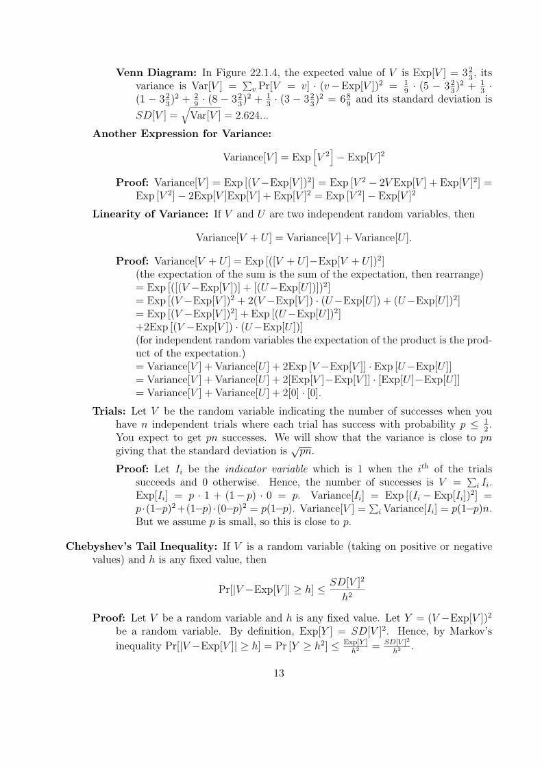
Venn Diagram: In Figure 22.1.4, the expected value of V is Exp[V ] = 323, its
variance is Var[V ] =∑
v Pr[V = v] · (v−Exp[V ])2 = 19· (5 − 32
3)2 + 1
3·
(1 − 323)2 + 2
9· (8 − 32
3)2 + 1
3· (3 − 32
3)2 = 68
9and its standard deviation is
SD[V ] =√Var[V ] = 2.624...
Another Expression for Variance:
Variance[V ] = Exp[V 2]− Exp[V ]2
Proof: Variance[V ] = Exp [(V −Exp[V ])2] = Exp [V 2 − 2V Exp[V ] + Exp[V ]2] =Exp [V 2]− 2Exp[V ]Exp[V ] + Exp[V ]2 = Exp [V 2]− Exp[V ]2
Linearity of Variance: If V and U are two independent random variables, then
Variance[V + U ] = Variance[V ] + Variance[U ].
Proof: Variance[V + U ] = Exp [([V + U ]−Exp[V + U ])2](the expectation of the sum is the sum of the expectation, then rearrange)= Exp [([(V −Exp[V ])] + [(U−Exp[U ])])2]= Exp [(V −Exp[V ])2 + 2(V −Exp[V ]) · (U−Exp[U ]) + (U−Exp[U ])2]= Exp [(V −Exp[V ])2] + Exp [(U−Exp[U ])2]+2Exp [(V −Exp[V ]) · (U−Exp[U ])](for independent random variables the expectation of the product is the prod-uct of the expectation.)= Variance[V ] + Variance[U ] + 2Exp [V −Exp[V ]] · Exp [U−Exp[U ]]= Variance[V ] + Variance[U ] + 2[Exp[V ]−Exp[V ]] · [Exp[U ]−Exp[U ]]= Variance[V ] + Variance[U ] + 2[0] · [0].
Trials: Let V be the random variable indicating the number of successes when youhave n independent trials where each trial has success with probability p ≤ 1
2.
You expect to get pn successes. We will show that the variance is close to pngiving that the standard deviation is
√pn.
Proof: Let Ii be the indicator variable which is 1 when the ith of the trialssucceeds and 0 otherwise. Hence, the number of successes is V =
∑i Ii.
Exp[Ii] = p · 1 + (1− p) · 0 = p. Variance[Ii] = Exp [(Ii − Exp[Ii])2] =
p ·(1−p)2+(1−p) ·(0−p)2 = p(1−p). Variance[V ] =∑
i Variance[Ii] = p(1−p)n.But we assume p is small, so this is close to p.
Chebyshev’s Tail Inequality: If V is a random variable (taking on positive or negativevalues) and h is any fixed value, then
Pr[|V −Exp[V ]| ≥ h] ≤ SD[V ]2
h2
Proof: Let V be a random variable and h is any fixed value. Let Y = (V −Exp[V ])2
be a random variable. By definition, Exp[Y ] = SD[V ]2. Hence, by Markov’s
inequality Pr[|V −Exp[V ]| ≥ h] = Pr [Y ≥ h2] ≤ Exp[Y ]h2 = SD[V ]2
h2 .
13
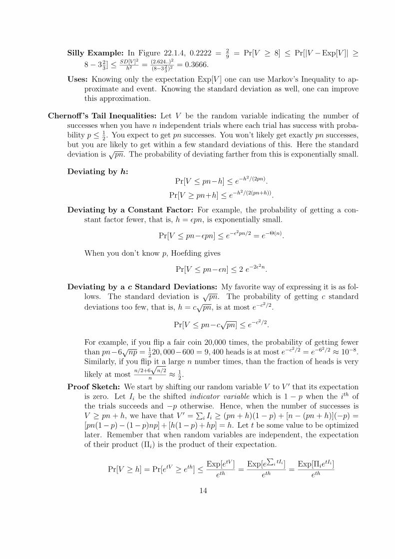
Silly Example: In Figure 22.1.4, 0.2222 = 29= Pr[V ≥ 8] ≤ Pr[|V −Exp[V ]| ≥
8− 323] ≤ SD[V ]2
h2 = (2.624..)2
(8−3 2
3)2
= 0.3666.
Uses: Knowing only the expectation Exp[V ] one can use Markov’s Inequality to ap-proximate and event. Knowing the standard deviation as well, one can improvethis approximation.
Chernoff’s Tail Inequalities: Let V be the random variable indicating the number ofsuccesses when you have n independent trials where each trial has success with proba-bility p ≤ 1
2. You expect to get pn successes. You won’t likely get exactly pn successes,
but you are likely to get within a few standard deviations of this. Here the standarddeviation is
√pn. The probability of deviating farther from this is exponentially small.
Deviating by h:Pr[V ≤ pn−h] ≤ e−h2/(2pn).
Pr[V ≥ pn+h] ≤ e−h2/(2(pn+h)).
Deviating by a Constant Factor: For example, the probability of getting a con-stant factor fewer, that is, h = ǫpn, is exponentially small.
Pr[V ≤ pn−ǫpn] ≤ e−ǫ2pn/2 = e−Θ(n).
When you don’t know p, Hoefding gives
Pr[V ≤ pn−ǫn] ≤ 2 e−2ǫ2n.
Deviating by a c Standard Deviations: My favorite way of expressing it is as fol-lows. The standard deviation is
√pn. The probability of getting c standard
deviations too few, that is, h = c√pn, is at most e−c2/2.
Pr[V ≤ pn−c√pn] ≤ e−c2/2.
For example, if you flip a fair coin 20,000 times, the probability of getting fewerthan pn−6
√np = 1
220, 000−600 = 9, 400 heads is at most e−c2/2 = e−62/2 ≈ 10−8.
Similarly, if you flip it a large n number times, than the fraction of heads is very
likely at mostn/2+6
√n/2
n≈ 1
2.
Proof Sketch: We start by shifting our random variable V to V ′ that its expectationis zero. Let Ii be the shifted indicator variable which is 1 − p when the ith ofthe trials succeeds and −p otherwise. Hence, when the number of successes isV ≥ pn + h, we have that V ′ =
∑i Ii ≥ (pn + h)(1 − p) + [n − (pn + h)](−p) =
[pn(1− p)− (1− p)np] + [h(1− p)+hp] = h. Let t be some value to be optimizedlater. Remember that when random variables are independent, the expectationof their product (Πi) is the product of their expectation.
Pr[V ≥ h] = Pr[etV ≥ eth] ≤ Exp[etV ]
eth=
Exp[e∑
itIi ]
eth=
Exp[ΠietIi ]
eth
14
=ΠiExp[e
tIi ]
eth=
Πi[p · et·(1−p) + (1−p) · et·(−p)]
eth=
[pet + (1−p)]n
eth+tpn
Because this is true for every choices of t, one just has to set t to minimize thisprobability.
Probability of Succeeding at Least Once: Suppose that that your experiment, say therunning of an algorithm, succeeds with at least probability p. Suppose that you are ableto repeat the experiment independently N times and that you only need to succeed atleast one of these times to succeed over all. Finally, suppose that you want to succeedoverall with probability 1− ǫ for some small ǫ > 0. Then it is sufficient to repeat theexperiment N = 1
pln(1ǫ
)times. The probability that you fail each of these times is at
mostPr[AlwaysFail] ≤ (1−p)N ≤ e−pN = e− ln( 1
ǫ ) = ǫ.
For example, if p = 1n2 and ǫ = 10−9 (one in a billion), thenN = 1
pln(1ǫ
)= n2 ln (109) ≤
21n2. See Exercise ??.
Probability of a Bad Event: Suppose that there is a list of bad things that might happen.Suppose that you can prove that the probability that the ith one happens is at mostpi. It follows that
Pr[At least one bad thing happens] ≤∑
i
pi
Proof: Suppose the probability that the ith bad thing happens is at mostpi. The worst case is when these bad events are disjoint so thattwo never occur simultaneously. Imagine a Venn diagram with dis-joint circles of area pi. In this case, the probability that one hap-pens is exactly
∑i pi. More formally, Pr[At least one bad thing happens] =
The # of r for which at least one bad thing happensThe # of r
≤ ∑iThe # of r for which the ith bad thing occurs
The # of r =∑
i pi.
Some Useful Approximations:
1 − p ≤ e−p: This is useful bound that we have seen already. It is very close toequality when p is close to zero, i.e. 1− 0 = 1 = e−0. Here are some other similarinequalities.
• 1− p+ p2
2≥ e−p
• 1 + p ≤ ep and for p ∈ [0, 1], 1 + p+ p2 ≥ ep and 1 + p ≥ ep−p2
3 .
• (1− p)n = 1− np+Θ(p2).
• 1 + p ≤ 11−p
and very close when p is small.
n! ≈(n
e
)n: This is a fairly close approximation of n! which is the number of ways
of arranging n objects. Stirling’s approximation, which is even closer, is n! =√eπn ·
(ne
)new where 1
12(n+.5)≤ w ≤ 1
12n.
15
(n
a
)a≤(n
a
)≤(en
a
)a: This is a fairly close approximation of
(na
)= n!
a!(n−a)!which is
the number of subsets of size a of n objects. Another approximation, which iseven closer is
(nrn
)≈ 2Entropy(r)·n, where Entropy(r) = r log2
1r+ (1−r) log2
11−r
.
Proofs:
1 + p ≤ ep and 1 − p ≤ e−p: These come from two formal definitions of the base ofnatural logarithms 2.718.., i.e. limN→∞(1+ 1
N)N = e and limN→∞(1− 1
N)N = e−1.
Also if you plot the two functions 1 + x and ex using the fact that the derivativeof both 1 + x and ex at zero is 1, you can see that 1 + x ≤ ex and similarly1− x ≤ e−x. These approximations are very close when x ∈ o(1).
1 + p + p2 ≥ ep and 1 − p + p2
2≥ e−p: The Taylor expansion of a function f(x)
at point x0 is a close approximation of f(x) for x close to x0. It is defined tobe f(x0 + p) ≈ f(x0) + f ′(x0)p + 1
2!f ′′(x0)p
2 + 13!f ′′′(x0)p
3 + . . .. Hence, ep ≈e0+ e0p+ 1
2!e0p2+ 1
3!e0p3+ . . . = 1+ p+ 1
2!p2+ 1
3!p3+ . . . ≤ 1+ p+ p2 when p ≤ 1.
Replacing p with −p gives e−p ≈ 1+ (−p) + 12!(−p)2 + 1
3!(−p)3 + . . . ≤ 1− p+ p2
2.
(1 − p)n = 1 − np + Θ(p2): You know that (1−p)2 = 1−2p+p2 and (1−p)3 = 1−3p+3p2− p3. More generally, (a+ b)n =
∑i = 0n
(ni
)an−ibi and hence (1− p)n =
∑i = 0n
(ni
)(−p)i = 1− np+ n2
2p2 −Θ(p3).
1 + p ≤ 11−p
: 11−p
= 1 + p+ p2 + p3 + . . .. The p2 become small when p is small.
n! ≈(n
e
)n: ln(n!) = ln(1·2·3·. . .·n) = ln(1)+ln(2)+ln(3)+. . .+ln(n) =
∑ni=1 ln(i) ≈
∫ ni=1 ln(i) = n ln(n)− n. Hence, n! = eln(n!) = en ln(n)−n =
[eln(n)
]n · e−n = nn
en.
(n
a
)a≤(n
a
)≤(en
a
)a:(na
)= n!
a!(n−a)!= n(n−1)(n−2)...(n−a+1)
a(a−1)(a−2)...1= n
a· n−1a−1
· n−2a−2
· . . . · n−a+11
≥(na
)a.(na
)= n!
a!(n−a)!= n(n−1)(n−2)...(n−a+1)
a!≤ na
a!≈ na
(a/e)a=(ena
)a.
Exercise 22.0.1 (See solution in Section ??) Prove that the two definitions of independentevents are equivalent, namely Pr[A|B] = Pr[A] and Pr[A and B] = Pr[A] · Pr[B].
Exercise 22.0.2 (See solution in Section ??) When A and B are independent, computePr[A and not B] and Pr[not A and not B] in terms of Pr[A] and Pr[B].
Exercise 22.0.3 (See solution in Section ??) Prove that these three definitions of Exp[V ]are equivalent.
Exercise 22.0.4 (See solution in Section ??) Suppose V is a random variable that onlytakes on values in the range [0,M ]. Use Markov’s inequality to prove the following.
• Pr[V < v] ≥ 1− Exp[V ]v
• Pr[V ≤ v] ≤ M−Exp[V ]M−v
• Pr[V > v] ≥ Exp[V ]−vM−v
16
Exercise Solutions
22.0.1 Clearly, the statement Pr[A|B] = Pr[A and B]Pr[B]
= Pr[A] is true if and only the state-
ment Pr[A and B] = Pr[A] · Pr[B] is true.
22.0.2 Pr[A and not B] = Pr[A]−Pr[A and B] = Pr[A]−Pr[A] ·Pr[B] = Pr[A] ·(1−Pr[B]).Pr[not A and not B] = Pr[not B] − Pr[A and not B] = (1 − Pr[B]) − Pr[A] · (1 −Pr[B]) = (1− Pr[A]) · (1− Pr[B])
22.0.3 Exp[V ] =∑
[disjoint events A]Pr[A] · [value of V during event A]
=∑
v
∑[disjoint events A for which V = v] Pr[A] · v
=∑
v Pr[V = v] · v.Obtaining the coin flips r is like an event A with Pr[A] = 1
The # of r . Hence,
Exp[V ] =∑disjoint events A
Pr[A] · [value of V during event A] =∑
r1
The # of r · Vr.
22.0.4 • Markov’s inequality is Pr[V ≥ v] ≤ Exp[V ]v
.
• The events V ≥ v and V < v are complementary events. Hence, Pr[V < v] =
1− Pr[V ≥ v], which by Markov’s inequality ≥ 1− Exp[V ]v
.
• Let W = M − V be how far V is from it’s maximum value. Note that W is arandom variable that only takes on non-negative values. Similarly, let w = M−v.Then Pr[V ≤ v] = Pr[M − V ≥ M − v] = Pr[W ≥ w], which by Markov’s
inequality ≤ Exp[W ]w
= M−Exp[V ]M−v
.
• The events V ≤ v and V > v are complementary events. Hence, Pr[V > v] =
1− Pr[V ≤ v], which by previous ≥ 1− M−Exp[V ]M−v
= Exp[V ]−vM−v
.
17
Chapter 23
Randomized Algorithms
For some computational problems, allowing the algorithm to flip coins (i.e. use a randomnumber generator) makes for a simpler, faster, makes for a simpler, faster, easier to analyzealgorithm. The following are the three main reasons.
Hiding the Worst Cases from the Adversary: The “running time” of a randomizedalgorithms is analyzed in a different way than that of a deterministic algorithm. Attimes, this way is more fair and more in line with how the algorithm actually performsin practice. Suppose, for example, that a deterministic algorithm quickly gives thecorrect answer on most input instances, yet is very slow or gives the wrong answeron a few instances. Its running time and its correctness is generally measured to bethat on these worst case instances. A randomized algorithm might also sometimes bevery slow or gives the wrong answer. See Quick Sort Section ??. However, we acceptthis, as long as on every input instance, the probability of doing so (over the choice ofrandom coins) is small.
Probabilistic Tools: The field of probabilistic analysis has many useful techniques andlemmas that can make the analysis of the algorithm simple and elegant.
Solution has a Random Structure: When the solution that we are attempting to con-struct has a random structure, a good way to construct it is to simply flip coins todecide how to built each part. Sometimes we are then able to prove that with highprobability the solution obtained this way has better properties than any solution weknow how to construct deterministically. Moreover, if we can prove that the solutionconstructed randomly has extremely good properties with some very small but non-zero probability, for example prob = 10−100, then this proves the existence of such asolution even though we have no reasonably quick way of finding one. Another inter-esting situation is when the randomly constructed solution very likely has the desiredproperties, for example with probability 0.999999, however, there is no quick way oftesting whether what we have produced has the desired properties.
This chapter considers these ideas further.
18

23.1 Using Randomness to Hide The Worst Cases
The standard way of measuring the running time and correctness of a deterministic algorithmis based on the worst case input instance chosen by some nasty adversary who has studied thealgorithm in detail. This is not fair if the algorithm does very well on all but a small numberof very strange and unlikely input instances. On the other hand, knowing that the algorithmworks well on most instances is not always satisfactory, because for some applications itis just those the hard instances that you want to solve. In such cases, it might be morecomforting to use a randomized algorithm that guarantees that on every input instance, thecorrect answer will be obtained quickly with high probability.
A randomized algorithm is able to flip coins as it proceeds to decide what actions to takenext. Equivalently, a randomized algorithm A can be thought of as a set of deterministicalgorithms A1, A2, A3, . . . where Ar is what algorithm A does when the outcome of the coinflips is r = 〈heads, tails, heads, heads, . . . , tails〉. Each such deterministic algorithm Ar willhave a small set of worst case input instances on which it either gives the wrong answer orruns too slow. The idea is that these algorithms A1, A2, A3, . . . have different sets of worstcase instances. This randomized algorithm is good if for each input instance, the fractionof the deterministic algorithms A1, A2, A3, . . . for which it is not a worst case instance is atleast p. Then when one of these Ar is chosen randomly, it solves this instance quickly withprobability at least p.
I sometimes find it useful to consider the analysis of randomized algorithms as a gamebetween an algorithm designer and an adversary who tries to construct input instance whichwill be bad for the algorithm. In the game, it is not always fair for the adversarial inputchooser to know the algorithm first, because then it can choose the instance that is worstcase for this algorithm. Similarly, it is not always fair for the algorithm designer to knowthe input instance first or even which instances are likely, because then it can design thealgorithm to work well on these. The way we analyze the running time of randomizedalgorithms compromises between these two. In this game, the algorithm designer withoutknowing the input instance must first fix what his algorithm will do given the outcome ofthe coins. Knowing this, but not knowing the outcomes of the coins, the instance chooserchooses the worst case instance. We then flip coins, run the algorithm, and see how well itdoes.
Three Models: The following are formal definitions of three models.
Deterministic Worst Case: In a worst case analysis, a deterministic algorithm Afor a computational problem P must always give the correct answer quickly.
∀I, [A(I) = P (I) and T ime(A, I) ≤ Tupper(|I|)]
Las Vegas: The algorithm is said to be Las Vegas if the algorithm is always guaranteedto give the correct answer, but the running time of the algorithm depends on theoutcomes of the random coin flips. The goal is to prove that on every inputinstance, the expected running time is small.
19
∀I, [∀r, Ar(I) = P (I) and Expr [T ime(Ar, I)]
≤ Tupper(|I|)]Monte Carlo: The algorithm is said to be Monte Carlo if the algorithm is guaranteed
to stop quickly, but it can sometimes, depending on the outcomes of the randomcoin flips, give the wrong answer. The goal is to prove that on every input, theprobability of it giving the wrong answer is small.
∀I, [Prr [Ar(I) 6= P (I)]
≤ pfails and ∀r, T ime(Ar, I)
≤ Tupper(|I|)]
The following examples demonstrate these ideas.
Quick Sort: Recall the quick sort algorithm from Section ??. The algorithm chooses a pivotelement and partitions the list of numbers to be sorted into those that are smaller thanthe pivot and those that are larger than it. Then it recurses on each of these two parts.The running time varies from Θ(n log n) to Θ(n2) depending on the choices of pivots.
Deterministic Worst Case: A reasonable choice for the pivot is to always use theelement that happens to be located in the middle of array to be sorted. For allpractical purposes, this would likely work great. It would work exceptionally wellwhen the list is already sorted. However, there are some strange inputs cookedups for the sole purpose of being nasty to this particular implementation of thealgorithm on which the algorithm runs in Θ(n2) time. The adversary will providesuch an input giving a worst case time complexity of Θ(n2).
Las Vegas: In practice, what is often done is to choose the pivot element randomlyfrom the input elements. This makes it irrelevant which order the adversary putsthe elements in the input instance. The expected computation time is Θ(nlogn).
The Game Show Problem: The input I to the game show problem specifies which of Ndoors has prizes behind them. At least half the doors are promised to have prizes. Analgorithm A is able to look behind the doors in any order that it likes, but nothingelse. It solves the problem correctly when it finds a prize. The running time is thenumber of doors opened.
Deterministic Worst Case: Any deterministic algorithm fixes the order that itlooks behind the doors. Knowing this order, the adversary places no prizes behindthe first N
2doors looked behind.
Las Vegas: In contrast, a random algorithm will look behind doors in random order.It does not matter where the adversary puts the prizes, the probability that oneis not found after t doors is 1
2tand the expected time until a prize is found is
Exp[T ] =∑
t Pr[T = t] · t = 2.
20
Monte Carlo: If the promise is that either at least half the doors have prizes or noneof them do and if the algorithm stops after 10 empty doors and claims that thereare no prizes, then this algorithm is always fast, but gives the wrong answer withprobability 1
210.
Randomized Primality Testing: An integer x is said to be composite if it has factorsother than one and itself. Otherwise, it is said to be prime. For example, 6 = 2 × 3is composite and 2, 3, 5, 7, 11, 13, 17, . . . are prime. See Appendix ?? Example 2 forexplanations of why it takes 2Θ(n) time to factor an n bit number.1 Here we give aneasy randomized algorithm by Rabin-Miller for this problem.
Fermat’s Little Theorem: Don’t worry about the math, but Fermat’s Little The-orem says that if x is prime, then for every a ∈ [1, x − 1], it is the case thatax−1 ≡(mod x) 1.
If we want to test if x is prime, then we can pick random a’s in the interval andsee if the equality holds. If the equality does not hold for a value of a, then x iscomposite. If the equality does hold for many values of a, then we can say that xis probably prime, or a what we call a pseudo prime.
The Game Show Problem: Finding an a for which ax−1 6≡(mod x) 1 is like finding aprize behind door a. See Exercise 23.1.1.
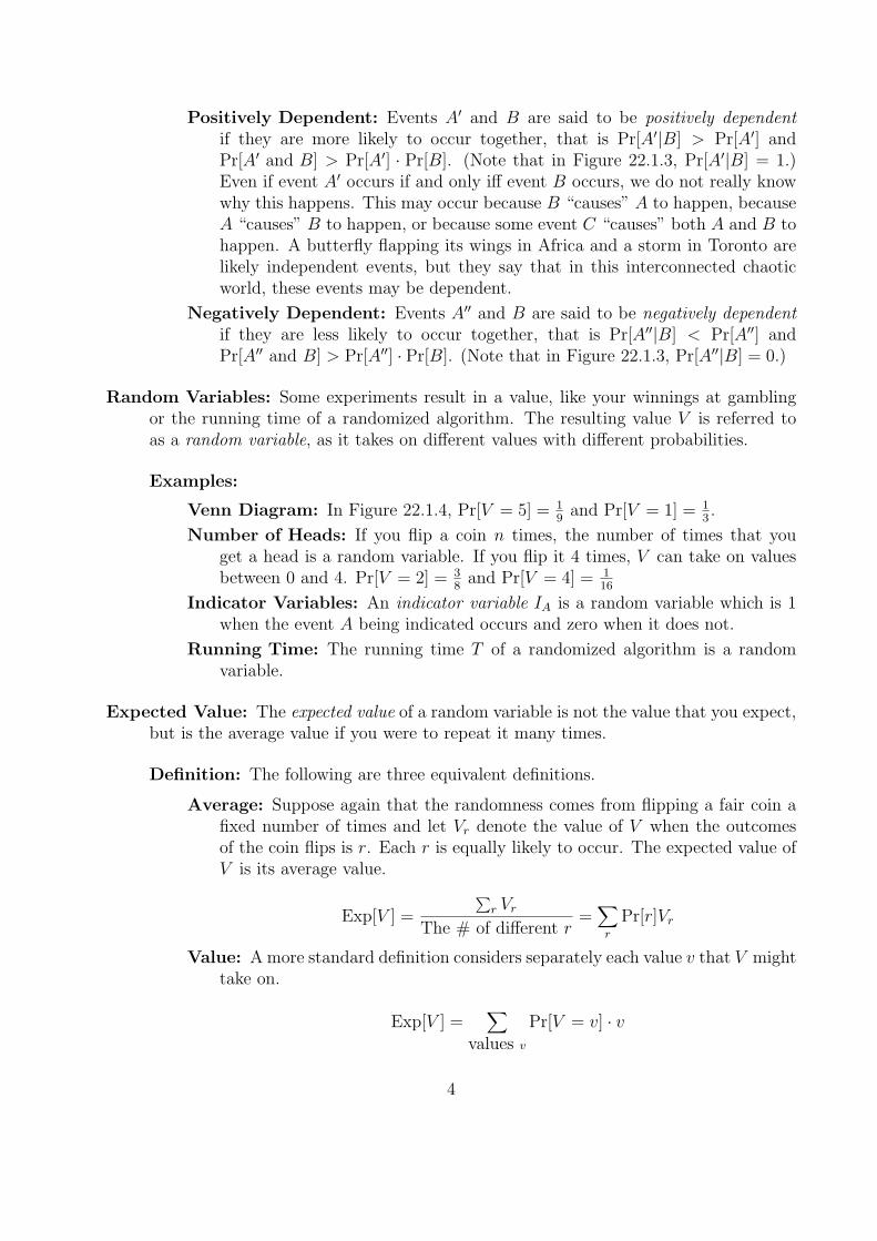
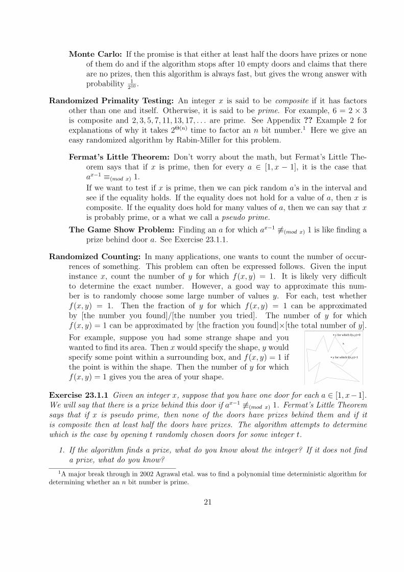
Randomized Counting: In many applications, one wants to count the number of occur-rences of something. This problem can often be expressed follows. Given the inputinstance x, count the number of y for which f(x, y) = 1. It is likely very difficultto determine the exact number. However, a good way to approximate this num-ber is to randomly choose some large number of values y. For each, test whetherf(x, y) = 1. Then the fraction of y for which f(x, y) = 1 can be approximatedby [the number you found]/[the number you tried]. The number of y for whichf(x, y) = 1 can be approximated by [the fraction you found]×[the total number of y].
For example, suppose you had some strange shape and youwanted to find its area. Then x would specify the shape, y wouldspecify some point within a surrounding box, and f(x, y) = 1 ifthe point is within the shape. Then the number of y for whichf(x, y) = 1 gives you the area of your shape.
y for which f(x,y)=0
y for which f(x,y)=1
x
Exercise 23.1.1 Given an integer x, suppose that you have one door for each a ∈ [1, x−1].We will say that there is a prize behind this door if ax−1 6≡(mod x) 1. Fermat’s Little Theoremsays that if x is pseudo prime, then none of the doors have prizes behind them and if itis composite then at least half the doors have prizes. The algorithm attempts to determinewhich is the case by opening t randomly chosen doors for some integer t.
1. If the algorithm finds a prize, what do you know about the integer? If it does not finda prize, what do you know?
1A major break through in 2002 Agrawal etal. was to find a polynomial time deterministic algorithm fordetermining whether an n bit number is prime.
21

2. If the algorithm must always give the correct answer, how many doors need to be openedin terms of the number of digits n in the instance x.
3. If t doors are open and the input instance x is a pseudo prime, what is the probabilitythat the algorithm gives the correct answer? If the instance is composite, what is thisprobability?
Exercise 23.1.2 Section ?? designed an iterative algorithm for separating n VLSI chipsinto those that are “good” and those that are “bad” by test two chips at a time and learningeither that they are the same or that they are different. To help, at least half of the chipsare promised to be good. Now design much easier a randomized algorithm for this problem.Here are some hints.
• Randomly select one of the chips. What is the probability that the chip is good?
• How can you learn whether or not the selected chip is good?
• If it is good, how can you easily partition the chips into good and bad chips.
• If the chip is not good, what should your algorithm do?
• When should the algorithm stop?
• What is the expected running time of this algorithm?
23.1.1 Sorry no answer
23.1.2 Sorry no answer
23.2 Locker Room Problem
Problem: There are n players, each with a locker and a driver’s license. The coach randomlypermutes the licenses and puts one in each locker. The players can agree on a strategy. Eachplayer independently goes into the locker room and can look in half the lockers. We saythat he succeed if he finds his own license. We say that they succeed if each player succeedsto finds his own license. They are not allowed to change the room set up or communicatein any way. The probability that a given player succeeds is 1
2. If things were completely
independent then the probability that all succeeds would be 12n. Is it possible for the players
to have a strategy in which they all succeed with a significantly higher probability, say 0.3?
Strategy: Each player starts by looking in his own locker. If he finds Bob’s license, he looksin Bob’s locker. If in Bob’s locker he finds John’s license, he looks in John’s locker next.This continues until either he finds his locker or has looked in half the lockers.
Permutation Graph: Put a directed edge from i to j if the locker i contains license j.Having out−degree one and in−degree one, this graph contains a collection of cycles.
Success: Player i starts at node i, i.e. his own locker, and follows the edges of this graph.He succeeds when he finds his own driver’s license, i.e. when the cycle he is following points
22

back to node i, i.e. he arrives back at node i. Hence, he succeeds when the cycle that he isin contains at most half the nodes. They all succeed if the permutation graph contains nocycles of length greater than half.
Probability of a k Cycle: Let k ∈ [n2+1, n]. We will show that the probability that a
random permutation graph contains a k cycle is 1k.
The number of permutation graphs is n! because it can be described by a permutation.There are n choices for a neighbor for node 1 and then n−1 choices for a neighbor for node2, because they can’t have the same neighbor, and so on.
Now let us count the number permutations with a cycle of length k. Choose a start nodei1. There are n ways. Choose its neighbor i2. There are n−1 ways, because we don’t wantto allow node i1. Choose i2’s neighbor i3. There are n−2 ways, because we don’t wantto allow nodes i1 or i2. Continue until you choose ik−1’s neighbor ik. There are n−(k−1)ways. Because we want a cycle of length k, we know that ik’s neighbor is node i1. Thenthere (n−k)! ways to arranging the remaining n−k players. The total number of ways is n!.However, we over counted by a factor of k because it does not matter which of the k nodesin the k cycle that we started with. Note that we would have over counted further if therewas a second cycle of length k in the remaining n−k nodes, but this is not possible becausen−k < k. Hence, the total number of permutation graphs with a cycle of length k is n!
k. The
fact that the probability is 1kfollows.
Probability of a Large Cycle: There can’t be two cycles of more than half the nodes.Hence, the event of there being a k cycle is disjoint for the different k ∈ [n
2+1, n]. Hence
the probability of there being a more than half cycle is∑n
k=n2+1
1k=∑n
k=11k−∑
n2
k=11k≈
ln(n)−ln(n2) = ln(2). Hence, the probability of no such large cycle and hence of success is
1−ln(2) > 0.3.
23.3 Solutions of Optimization Problems with a Ran-
dom Structure
Optimization problems are looking for the best solution for an instance. Sometimes goodsolutions have a random structure. In such cases, a good way to construct it is to simplyflip coins to decide how to built each part. We give two examples. The first one, Max Cut,being NP-complete, likely requires exponential time to find the best solution. However, inO(n) time, we can find a solution which is likely to be at least half as good as optimal.The second example, expander graphs is even more extreme. Though there are deterministicalgorithms for constructing graphs with fairly good expansion properties, a random graphalmost for sure has much better expansion properties (with probability p ≥ 0.999999). Acomplication, however, is that there is no polynomial time algorithm which tests whetherthis randomly constructed graph has the desired properties. Pushing the limits further, itcan be proved that the same random graph has extremely good properties with some verysmall but non-zero probability (eg. p ≥ 10−100). Though we have no quick way to constructsuch a graph, this does proves that such a graph exists.
23
The Max Cut Problem: The input to the Max Cut problem is an undirected graph. Theoutput is a partition of the nodes into two sets U and V so that the number of edgesthat cross over from one side to the other is as large as possible. This problem is NP-complete and hence, the best known algorithm for finding an optimal solution requires2Θ(n) time. The following randomized algorithm runs in time Θ(n) and is expectedto obtain a solution for which half the edges cross over. This algorithm is incrediblysimple. It simply flips a coin for each node to decide whether to put it into U or intoV . Each edge will cross over with probability 1
2. Hence, the expected number of edges
to cross over is |E|2. The optimal solution cannot have more than all the edges cross
over, so the randomized algorithm is expected to perform at least half as well as theoptimal solution can do.
Expander Graphs: An n node degree d graph is said to be an Expander Graph if movingfrom a set of its nodes across its edges expands us out to an even larger set of nodes.More formally, for 0 < α < 1 and 1 < β < d, a graph G = 〈V,E〉 is an 〈α, β〉-expanderif for every subset S ⊆ V of its nodes, if |S| ≤ αn then |N(S)| ≥ β|S|. Here N(S) isthe neighborhood of S, that is all nodes with an edge from some node in S.
Non-Overlapping Sets of d Neighbors: Because each node v ∈ V has d neighborsN(v), a set S has d|S| edges leaving these nodes. However, if these sets N(v) ofneighbors overlap a lot, then the total number of neighbors N(S) = ∪v∈SN(v)of S might be very small. We can’t expect N(S) to be bigger than d|S| but wedo want it to have size at least β|S| where 1 < β < d. If S is too big, we can’texpect it to expand further. Hence, we only require this expansion property forsets S of size at most αn. Because we do expect sets of size αn to expand to aneighborhood of size βαn, we do require that αβ < 1.
Connected with Short Paths: If αβ > 12, then every pair of nodes inG is connected
with a path of length at most 2 log(n/2)log β
.
Proof: Consider two nodes u and v. The node u has d neighbors, N(u). Theseneighbors N(u) must have at least β|N(u)| = βd neighbors N(N(u)). Theseneighbors N(N(u)) must have at least β2d neighbors. It follows that thereare at least βi−1d nodes with distance i from u. The last time we are allowto do this expands the neighbor set of size |S| = αn to |N(S)| ≥ β|S| = βαn.By the requirement that αβ > 1
2, this new neighbor set has size greater than
n2nodes. The distance of these nodes from u is at most i = logβ
n2. This set
might not contain v. However, starting from v there is another set of morethan half the nodes that are distance i = logβ
n2from v. These two sets must
over lap at some node w. Hence, there is a path from u to w to v of lengthat most 2 log(n/2)
log β.
Uses: Expander graphs are very useful both in practice and for proving theorems.
Fault Tolerant Networks: As we have seen every pair of nodes in an expandergraph are connected. This is still true if a large number of nodes or edgesfail. Hence, this is a good pattern for wiring a communications network.
24

Pseudo Random Generators: Taking a short random walk in an expandergraph quickly gets you to a random node. This is useful for generating longrandom looking strings from a short seed string.
Concentrating and Recycling Random Bits: If we have a source that hassome randomness in it (say n coin tosses with an unknown probability andwith unknown dependencies between the coins), we can use expander graphsto produce a string of m bits appearing to be the result of m fair and inde-pendent coins.
Error Correcting Codes: Expander graphs are also useful in designing waysof encoding a message into a longer code so that if any reasonable fraction ofthe longer code is corrupted, the original message can still be recovered. Thethe faulty bits are connected by short paths to correct bits.
If αβ < 1, then Expander Graphs Exists: We will now prove that for any constants αand β for which αβ < 1 there exists an 〈α, β〉-expander graph with n nodes and degreed for some sufficiently big constant d. For example, if α = 1
2, β = 3
2, then d = 5 is
sufficient. To make the analysis easier, we will consider directed graphs where eachnode u is connected to d nodes chosen independently at random. (If we ignore thedirections of the edges, then each node has average degree 2d and neighborhood setsare only bigger.) We prove that the probability we do not get such an expander graphis strictly less than one. Hence, one must exist.
Event ES,T : The graph G will not be a 〈α, β〉-expander if there is some set S forwhich |S| ≤ αn and N(S) < β|S|. Hence, for each pair of sets S and T , with|S| ≤ αn and |T | < β|S|, let ES,T denote the bad event that N(S) ⊆ T . Letus bound the probability of ES,T when we choose G randomly. Each node in Sneeds d neighbors for a total of d|S| randomly chosen neighbors. The probability
of a particular one of these landing in T is |T |n. Because these edges are chosen
independently, the probability of them all landing in T is(|T |n
)d|S|.
Probability of Some Bad Event: The probability that G is not an expander is theprobability that at least one of these bad events ES,T happens, which is at mostthe sum of the probabilities of these individual events.
Pr [G not an expander] = Pr [At least one of the events ES,T occurs] ≤∑
S,T
Pr [ES,T ]
=∑
(s≤αn)
∑
(S | |S|=s)
∑
(T | |T |=βs)
Pr [ES,T ] =∑
s≤αn
(n
s
)(n
βs
)( |T |n
)d|S|
We now use the result that(na
)≤(ena
)a.
Pr [G not an expander] ≤∑
s≤αn
(en
s
)s (enβs
)βs (βsn
)ds
=∑
s≤αn
[(en
s
)(en
βs
)β (βsn
)d]s
≤∑
s≤αn
[(en
αn
)(en
βαn
)β (βαnn
)d]s
=∑
s≤αn
[eβ+1
α· (αβ)d−β
]s
25

The requirement is that αβ < 1. Hence, if d is sufficiently big,(d ≥ log
(2eβ+1
α
)/ log
(1αβ
)+ β
), then the bracketed amount is at most 1
2.
Pr [G not an expander] ≤∑
s≤αn
[1
2
]s< 1
It follows that Pr [G is an expander] > 0, meaning that there exists at least onesuch G which is an expander.
26