Embed Size (px)
Citation preview
Chapter 21 1
Chapter 21
What Is a Confidence Interval?
Chapter 21 2
Thought Question 1
Suppose that 40% of a certain population favor the use of nuclear power for energy.
(a) If you randomly sample 10 people from this population, will exactly four (40%) of them be in favor of the use of nuclear power? Would you be surprised if only two (20%) of them are in favor? How about if none of the sample are in favor?

Chapter 21 3
Thought Question 2
(b) Now suppose you randomly sample 1000 people from this population. Will exactly 400 (40%) of them be in favor of the use of nuclear power? Would you be surprised if only 200 (20%) of them are in favor? How about if none of the sample are in favor?
Suppose that 40% of a certain population favor the use of nuclear power for energy.

Chapter 21 4
Thought Question 3
A 95% confidence interval for the proportion of adults in the U.S. who have diabetes extends from .07 to .11, or 7% to 11%. What does it mean to say that the interval from .07 to .11 represents a 95% confidence interval for the proportion of adults in the U.S. who have diabetes ?
Chapter 21 5
Thought Question 4
Would a 99% confidence interval for the proportion described in Question 3 be wider or narrower than the 95% interval given? Explain. (Hint: what is the difference between a 68% interval and a 95% interval?)

Chapter 21 6
Thought Question 5
In a May 2006 Zogby America poll of 1000 adults, 70% said that past efforts to enforce immigration laws have been inadequate. Based on this poll, a 95% confidence interval for the proportion in the population who feel this way is about 67% to 73%. If this poll had been based on 5000 adults instead, would the 95% confidence interval be wider or narrower than the interval given? Explain.

Chapter 21 7
Recall from previous chapters:Parameter
fixed, unknown number that describes the population
Statisticknown value calculated from a samplea statistic is used to estimate a parameter
Sampling Variabilitydifferent samples from the same population may yield different values of the sample statisticestimates from samples will be closer to the true values in the population if the samples are larger

Chapter 21 8
Recall from previous chapters:
Sampling Distributiontells what values a statistic takes and how often it takes those values in repeated sampling.
Example:sample proportions ( ’s) from repeated sampling would have a normal distribution with a certain mean and standard deviation.
p̂
Example:The amount by which the proportion obtained from the sample ( ) will differ from the true population proportion (p) rarely exceeds the margin of error.
p̂

Chapter 21 9
Case Study
Science News, Jan. 27, 1995, p. 451.
Comparing Fingerprint Patterns

Chapter 21 10
Case Study: Fingerprints Fingerprints are a “sexually dimorphic trait…
which means they are among traits that may be influenced by prenatal hormones.”
It is known…– Most people have more ridges in the fingerprints
of the right hand. (People with more ridges in the left hand have “leftward asymmetry.”)
– Women are more likely than men to have leftward asymmetry.
Compare fingerprint patterns of heterosexual and homosexual men.

Chapter 21 11
66 homosexual men were studied.• 20 (30%) of the homosexual men showed
left asymmetry.
186 heterosexual men were also studied• 26 (14%) of the heterosexual men showed
left asymmetry.
Case Study: FingerprintsStudy Results

Chapter 21 12
Case Study: FingerprintsA Question
Assume that the proportion of all men
who have leftward asymmetry is 15%.
Is it unusual to observe a sample of 66 men with a sample
proportion ( ) of 30% if the true population proportion (p) is 15%?
p̂

Chapter 21 13
Twenty Simulated Samples (n=66)
0
0.1
0.2
0.3
0.4
0.5
0.6
0.7
0.8
0.9
1
1 6 11 16 21 26 31 36 41 46 51 56 61 66 71 76 81 86 91 96
Sample Size
Obs
erve
d P
rop o
r tio
n

Chapter 21 14
The Rule for Sample Proportions
If numerous simple random samples of size n are taken from the same population, the sample proportions from the various samples will have an approximately normal distribution. The mean of the sample proportions will be p (the true population proportion). The standard deviation will be:
n
pp )1(
)ˆ( p

Chapter 21 15
Rule Conditions and Illustration
For rule to be valid, must have Random sample ‘Large’ sample size

Chapter 21 16
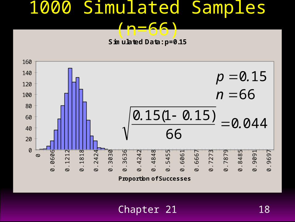
s.d.) ( 0440 66
)1501(150)1(
66 mean); ( 150
.
..n
pp
n.p
Case Study: FingerprintsSampling Distribution
Chapter 21 17
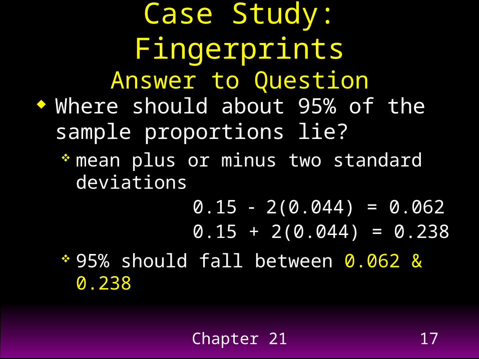
Case Study: FingerprintsAnswer to Question
Where should about 95% of the sample proportions lie? mean plus or minus two standard deviations
0.15 2(0.044) = 0.0620.15 + 2(0.044) = 0.238
95% should fall between 0.062 & 0.238
Chapter 21 18
Simulated Data: p=0.15
0
20
40
60
80
100
120
140
160
0
0.06
06
0.12
12
0.18
18
0.24
24
0.30
30
0.36
36
0.42
42
0.48
48
0.54
55
0.60
61
0.66
67
0.72
73
0.78
79
0.84
85
0.90
91
0.96
97
Proportion of Successes
1000 Simulated Samples (n=66)
044066
)1501(150
66150
...
n.p

Chapter 21 19
Simulated Data: p=0.15
0
20
40
60
80
100
120
140
160
0
0.06
06
0.12
12
0.18
18
0.24
24
0.30
30
0.36
36
0.42
42
0.48
48
0.54
55
0.60
61
0.66
67
0.72
73
0.78
79
0.84
85
0.90
91
0.96
97
Proportion of Successes
1000 Simulated Samples (n=66)
approximately 95% of sample proportions fall in this interval(0.062 to 0.238).
Is it likely we would observea sample proportion 0.30?

Chapter 21 20
Simulated Data: p=0.15
0
20
40
60
80
100
120
140
160
180
200
0
0.06
67
0.13
33
0.20
00
0.26
67
0.33
33
0.40
00
0.46
67
0.53
33
0.60
00
0.66
67
0.73
33
0.80
00
0.86
67
0.93
33
Proportion of Successes
1000 Simulated Samples (n=30)
065030
)1501(150
30150
...
n.p

Chapter 21 21
Simulated Data: p=0.15
0
20
40
60
80
100
120
140
160
180
200
0
0.06
67
0.13
33
0.20
00
0.26
67
0.33
33
0.40
00
0.46
67
0.53
33
0.60
00
0.66
67
0.73
33
0.80
00
0.86
67
0.93
33
Proportion of Successes
1000 Simulated Samples (n=30)
approximately 95% of sample proportions fall in this interval.
Is it likely we would observea sample proportion 0.30?
Chapter 21 22
Confidence Interval for a Population Proportion
An interval of values, computed from sample data, that is almost sure to cover the true population proportion.
“We are ‘highly confident’ that the true population proportion is contained in the calculated interval.”
Statistically (for a 95% C.I.): in repeated samples, 95% of the calculated confidence intervals should contain the true proportion.

Chapter 21 23
since we do not know the population proportion p (needed to calculate the standard deviation) we will use the sample proportion in its place.
Formula for a 95% Confidence Interval for the Population
Proportion (Empirical Rule) sample proportion plus or minus
two standard deviations ofthe sample proportion:
p̂
n)p(p
p̂ 1
2

Chapter 21 24
n
ppp
)ˆ1(ˆ2ˆ
standard error (estimated standard deviation of )p̂
Formula for a 95% Confidence Interval for the Population
Proportion (Empirical Rule)

Chapter 21 25
Margin of Error
nn
..
n
p̂p̂
1)501(50
)1(
2
2
(plus or minus part of C.I.)

Chapter 21 26
Formula for a C-level (%) Confidence Interval for the Population Proportion
npp
p z )ˆ1(ˆˆ *
where z* is the critical value of the standard normal distribution for confidence level C

Chapter 21 27
Common Values of z*Confidence Level
CCritical Value
z*50% 0.67
60% 0.84
68% 1
70% 1.04
80% 1.28
90% 1.64
95% 1.96 (or 2)
99% 2.58
99.7% 3
99.9% 3.29

Chapter 21 28
Case Study
Brown, C. S., (1994) “To spank or not to spank.” USA Weekend, April 22-24, pp. 4-7.
Parental Discipline
What are parents’ attitudes and practices on discipline?

Chapter 21 29
Case Study: Survey
Parental Discipline Nationwide random telephone survey of
1,250 adults.– 474 respondents had children under 18
living at home– results on behavior based on the smaller
sample reported margin of error
– 3% for the full sample– 5% for the smaller sample

Chapter 21 30
Case Study: Results
Parental Discipline “The 1994 survey marks the first time a
majority of parents reported not having physically disciplined their children in the previous year. Figures over the past six years show a steady decline in physical punishment, from a peak of 64 percent in 1988”– The 1994 proportion who did not spank or
hit was 51% !

Chapter 21 31
Case Study: Results
Parental Discipline Disciplining methods over the past year:
– denied privileges: 79%– confined child to his/her room: 59%– spanked or hit: 49%– insulted or swore at child: 45%
Margin of error: 5%– Which of the above appear to show a true
value different from 50%?

Chapter 21 32
Case Study: Confidence Intervals
Parental Discipline denied privileges: 79%
– : 0.79– standard error of : – 95% C.I.: .79 2(.019) : (.752, .828)
confined child to his/her room : 59%– : 0.59– standard error of : – 95% C.I.: .59 2(.023) : (.544, .636)
0190474)791(79 ...
0230474)591(59 ...
p̂p̂
p̂p̂
Chapter 21 33
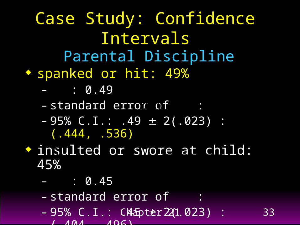
Case Study: Confidence Intervals
Parental Discipline spanked or hit: 49%
– : 0.49– standard error of : – 95% C.I.: .49 2(.023) : (.444, .536)
insulted or swore at child: 45%– : 0.45– standard error of : – 95% C.I.: .45 2(.023) : (.404, .496)
0230474)491(49 ...
0230474)451(45 ...
p̂p̂
p̂p̂

Chapter 21 34
Case Study: Results
Parental Discipline Asked of the full sample (n=1,250):
“How often do you think repeated yelling or swearing at a child leads to long-term emotional problems?”– very often or often: 74%– sometimes: 17%– hardly ever or never: 7%– no response: 2%
Margin of error: 3%

Chapter 21 35
Case Study: Confidence Intervals
Parental Discipline hardly ever or never: 7%
– : 0.07– standard error of : – 95% C.I.: .07 2(.007) : (.056, .084)
Few people believe such behavior is harmless, but almost half (45%) of parents engaged in it!
00701250)071(07 ...
p̂p̂

Chapter 21 36
Key Concepts (1st half of Ch. 21)
Different samples (of the same size) will generally give different results.
We can specify what these results look like in the aggregate.
Rule for Sample Proportions Compute and interpret Confidence
Intervals for population proportions based on sample proportions

Chapter 21 37
Inference for Population MeansSampling Distribution, Confidence Intervals
The remainder of this chapter discusses the situation when interest is in making conclusions about population means rather than population proportions– includes the rule for the sampling distribution
of sample means ( )– includes confidence intervals for one mean
or a difference in two means
s'X
Chapter 21 38
Thought Question 6(from Seeing Through Statistics, 2nd Edition, by Jessica M. Utts, p. 316)
Suppose the mean weight of all women at a university is 135 pounds, with a standard deviation of 10 pounds.
• Recalling the material from Chapter 13 about bell-shaped curves, in what range would you expect 95% of the women’s weights to fall? 115 to 155 pounds

Chapter 21 39
Thought Question 6 (cont.)
• If you were to randomly sample 10 women at the university, how close do you think their average weight would be to 135 pounds?
• If you randomly sample 1000 women, would you expect the average to be closer to 135 pounds than it would be for the sample of 10 women?

Chapter 21 40
Thought Question 7
A study compared the serum HDL cholesterol levels in people with low-fat diets to people with diets high in fat intake. From the study, a 95% confidence interval for the mean HDL cholesterol for the low-fat group extends from 43.5 to 50.5...
a. Does this mean that 95% of all people with low-fat diets will have HDL cholesterol levels between 43.5 and 50.5? Explain.

Chapter 21 41
Thought Question 7 (cont.)
… a 95% confidence interval for the mean HDL cholesterol for the low-fat group extends from 43.5 to 50.5. A 95% confidence interval for the mean HDL cholesterol for the high-fat group extends from 54.5 to 61.5.
b. Based on these results, would you conclude that people with low-fat diets have lower HDL cholesterol levels, on average, than people with high-fat diets?
( ) ( )40 45 50 55 60 65

Chapter 21 42
Thought Question 8
The first confidence interval in Question 7 was based on results from 50 people. The confidence interval spans a range of 7 units. If the results had been based on a much larger sample, would the confidence interval for the mean cholesterol level have been wider, more narrow or about the same? Explain.

Chapter 21 43
Thought Question 9
In Question 7, we compared average HDL cholesterol levels for two diet groups by computing separate confidence intervals for the two means. Is there a more direct value (and single C.I.) to examine in order to make the comparison between the two groups?
Chapter 21 44
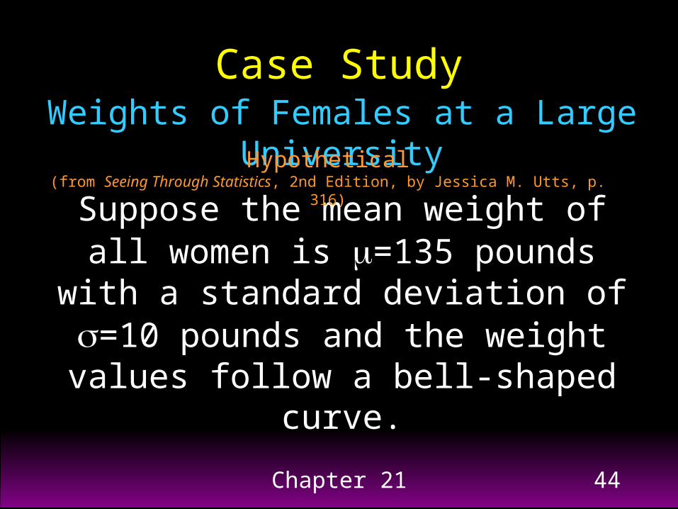
Case Study
Weights of Females at a Large University
Suppose the mean weight of all women is =135 pounds with a
standard deviation of =10 pounds and the weight values follow a bell-
shaped curve.
Hypothetical(from Seeing Through Statistics, 2nd Edition, by Jessica M. Utts, p. 316)

Chapter 21 45
What about the mean (average) of a sample of n women? What values would be expected?
Case Study: WeightsQuestions
Where should 95% of all women’s weights fall? mean plus or minus two standard deviations
135 2(10) = 115
135 + 2(10) = 155 95% should fall between 115 & 155

Chapter 21 46
Twenty Simulated Samples (n=1000)
130
131
132
133
134
135
136
137
138
139
140
1 6 11 16 21 26 31 36 41 46 51 56 61 66 71 76 81 86 91 96Sample Size
Obs
erve
d M
ean
We i
ght
1 500 1000

Chapter 21 47
The Rule for Sample Means
If numerous simple random samples of size n
are taken from the same population, the sample
means from the various samples will have
an approximately normal distribution. The
mean of the sample means will be (the
population mean). The standard deviation will
be: ( is the population s.d.)n
)(X

Chapter 21 48
Conditions for the Rule for Sample Means
Random sample Population of measurements…
– Follows a bell-shaped curve
- or -
– Not bell-shaped, but sample is ‘large’

Chapter 21 49
)X for s.d. ( 3.1610
10
10
)population for s.d. ( 10
)X and population for mean ( 135
nσ
n
σ
μ
Case Study: Weights Sampling Distribution
(for n = 10)
Chapter 21 50
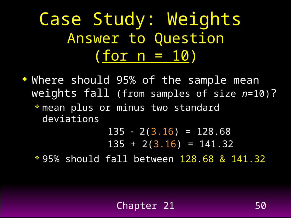
Where should 95% of the sample mean weights fall (from samples of size n=10)? mean plus or minus two standard deviations
135 2(3.16) = 128.68 135 + 2(3.16) = 141.32
95% should fall between 128.68 & 141.32
Case Study: Weights Answer to Question
(for n = 10)
Chapter 21 51
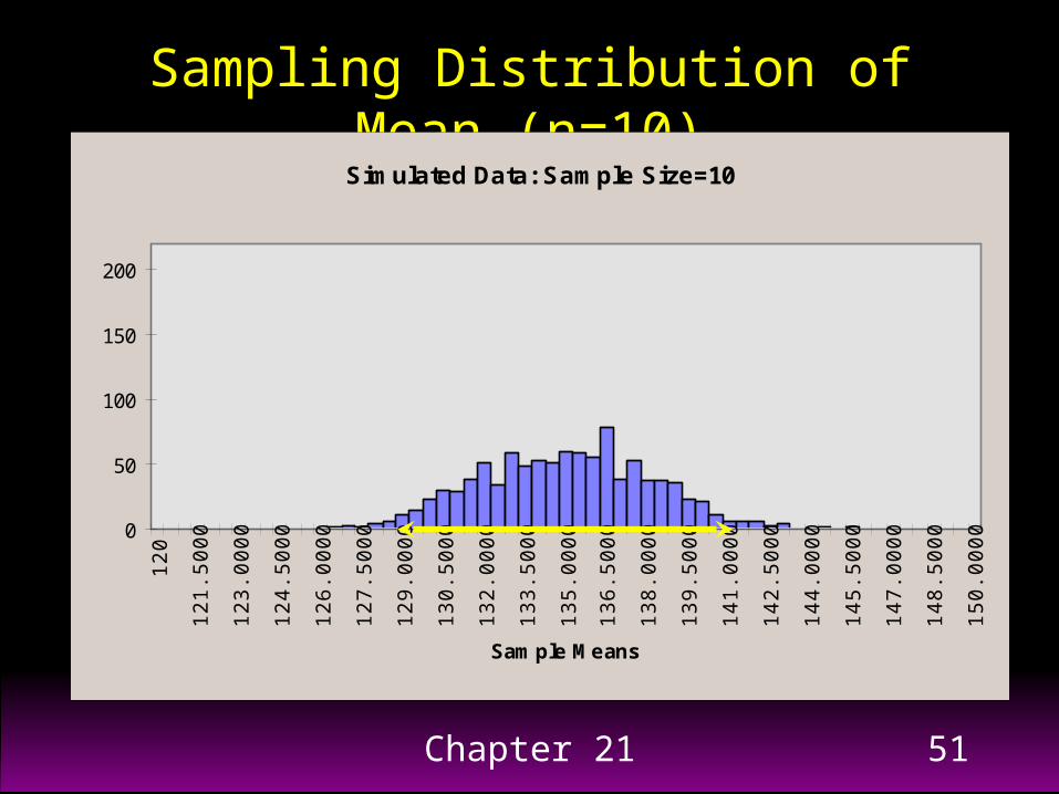
Sampling Distribution of Mean (n=10)Simulated Data: Sample Size=10
0
50
100
150
200
120
121.
5000
123.
0000
124.
5000
126.
0000
127.
5000
129.
0000
130.
5000
132.
0000
133.
5000
135.
0000
136.
5000
138.
0000
139.
5000
141.
0000
142.
5000
144.
0000
145.
5000
147.
0000
148.
5000
150.
0000
Sample Means

Chapter 21 52
225
10
25
10
135
n
σ
μ
Case Study: Weights Sampling Distribution
(for n = 25)

Chapter 21 53
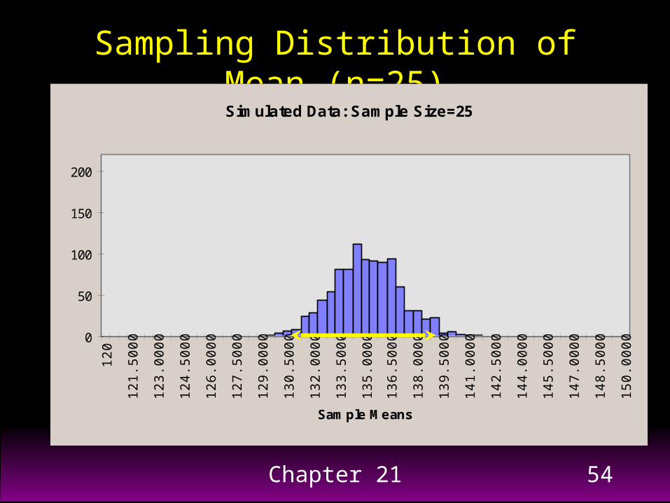
Where should 95% of the sample mean weights fall (from samples of size n=25)? mean plus or minus two standard deviations
135 2(2) = 131 135 + 2(2) = 139
95% should fall between 131 & 139
Case Study: Weights Answer to Question
(for n = 25)
Chapter 21 54
Sampling Distribution of Mean (n=25)Simulated Data: Sample Size=25
0
50
100
150
200
120
121.
5000
123.
0000
124.
5000
126.
0000
127.
5000
129.
0000
130.
5000
132.
0000
133.
5000
135.
0000
136.
5000
138.
0000
139.
5000
141.
0000
142.
5000
144.
0000
145.
5000
147.
0000
148.
5000
150.
0000
Sample Means

Chapter 21 55
1100
10
100
10σ
135
n
μ
Case Study: Weights Sampling Distribution
(for n = 100)

Chapter 21 56
Where should 95% of the sample mean weights fall (from samples of size n=100)? mean plus or minus two standard deviations
135 2(1) = 133 135 + 2(1) = 137
95% should fall between 133 & 137
Case Study: Weights Answer to Question
(for n = 100)

Chapter 21 57
Sampling Distribution of Mean (n=100)Simulated Data: Sample Size=100
0
50
100
150
200
120
121.
5000
123.
0000
124.
5000
126.
0000
127.
5000
129.
0000
130.
5000
132.
0000
133.
5000
135.
0000
136.
5000
138.
0000
139.
5000
141.
0000
142.
5000
144.
0000
145.
5000
147.
0000
148.
5000
150.
0000
Sample Means

Chapter 21 58
Case Study
Hypothetical
Exercise and Pulse Rates
Is the mean resting pulse rate of adult subjects who regularly exercise different
from the mean resting pulse rate of those who do not regularly exercise?
Find Confidence Intervals for the means

Chapter 21 59
n mean std. dev. Nonexercisers 31 75 9.0 Exercisers 29 66 8.6
Case Study: Results
Exercise and Pulse RatesA random sample of n1=31 nonexercisers yielded a sample
mean of =75 beats per minute (bpm) with a sample standard deviation of s1=9.0 bpm. A random sample of
n2=29 exercisers yielded a sample mean of =66 bpm
with a sample standard deviation of s2=8.6 bpm.
1X
2X

Chapter 21 60
The Rule for Sample Means
If numerous simple random samples of size n
are taken from the same population, the sample
means from the various samples will have
an approximately normal distribution. The
mean of the sample means will be (the
population mean). The standard deviation will
be:n
)(X
We do not know the value of !
Chapter 21 61
Standard Error of the (Sample) Mean
SEM = standard error of the mean
(standard deviation from the sample) = divided by
(square root of the sample size)
= ns

Chapter 21 62
Case Study: Results
Exercise and Pulse Rates n mean std. dev. std. err. Nonexer. 31 75 9.0 1.6 Exercisers 29 66 8.6 1.6
Typical deviation of an individual pulse rate(for Exercisers) is s = 8.6
Typical deviation of a mean pulse rate(for Exercisers) is = 1.6
ns
298.6

Chapter 21 63
Case Study: Confidence Intervals
Exercise and Pulse Rates
Nonexercisers: 75 ± 2(1.6) = 75 ± 3.2 = (71.8, 78.2)
Exercisers: 66 ± 2(1.6) = 66 3.2 = (62.8, 69.2)
Do you think the population means are different?
95% C.I. for the population mean: sample mean 2 (standard error)
X ns
2
Yes, because the intervals do not overlap

Chapter 21 64
Formula for a C-level (%) Confidence Interval for the Population Mean
* sxn
z
where z* is the critical value of the standard normal distribution for confidence level C

Chapter 21 65
Careful Interpretation of a Confidence Interval
“We are 95% confident that the mean resting pulse rate for the population of all exercisers is between 62.8 and 69.2 bpm.” (We feel that plausible values for the population of exercisers’ mean resting pulse rate are between 62.8 and 69.2.)
** This does not mean that 95% of all people who exercise regularly will have resting pulse rates between 62.8 and 69.2 bpm. **
Statistically: 95% of all samples of size 29 from the population of exercisers should yield a sample mean within two standard errors of the population mean; i.e., in repeated samples, 95% of the C.I.s should contain the true population mean.

Chapter 21 66
Exercise and Pulse Rates 95% C.I. for the difference in population
means (nonexercisers minus exercisers): (difference in sample means)
2 (SE of the difference) Difference in sample means: = 9 SE of the difference = 2.26 (given) 95% confidence interval: (4.48, 13.52)
– interval does not include zero ( means are different)
1 2X X
Case Study: Confidence Intervals

Chapter 21 67
An Experiment Testing a Vaccine for Those with Genital Herpes
Case Study
Adler, T., (1994) “Therapeutic vaccine fights herpes.” Science News, Vol. 145, June 18, p. 388.
Does a new vaccine prevent the outbreak of herpes in people already
infected?

Chapter 21 68
An Experiment Testing a Vaccine for Those with Genital Herpes
Case Study: Sample
98 men and women aged 18 to 55 Experience between 4 and 14
outbreaks per year Experiment
– Double-blind experiment– Randomized to vaccine or placebo

Chapter 21 69
An Experiment Testing a Vaccine for Those with Genital Herpes
Case Study: Report
“The vaccine was well tolerated. gD2 recipients reported fewer recurrences per month than placebo recipients (mean 0.42 [sem 0.05] vs 0.55 [0.05]…)…”

Chapter 21 70
An Experiment Testing a Vaccine for Those with Genital Herpes
Case Study: Confidence Intervals
95% C.I. for population mean recurrences:– Vaccine group: 0.42 2(0.05) : (.32, .52)– Placebo group: 0.55 2(0.05) : (.45, .65)
95% C.I. for the difference in population means:– Difference = -0.13, SE = 0.07 (given)
– C.I.: (-0.27, 0.01) (contains 0 means not different)

Chapter 21 71
Key Concepts (2nd half of Ch. 21)
Rule for Sample Means Compute confidence intervals for means
based on one sample Compute confidence intervals for means
based on two samples
Interpret Confidence Intervals for Means


![[--------------------- ---------------------] Chapter 8 Interval Estimation n Interval Estimation of a Population Mean: Large-Sample Case Large-Sample](https://img.dokumen.tips/doc/110x75/56649e895503460f94b8e9b8/-chapter-8-interval-estimation.jpg)


![Optimization - Cornell University · Bisection Method • Suppose we have an interval [a,b] and we would like to find a local minimum in that interval. • Evaluate at c = (a+b)/2](https://img.dokumen.tips/doc/110x75/5e87e51f84a8712c5b02b12e/optimization-cornell-bisection-method-a-suppose-we-have-an-interval-ab-and.jpg)