Chapter 21

Kinetic Theory of Warm Plasmas

Version 0221.1.pdf, 09 April 2003.Please send comments, suggestions, and errata via email to kip@tapir.caltech.edu and alsoto rdb@caltech.edu, or on paper to Kip Thorne, 130-33 Caltech, Pasadena CA 91125

21.1 Overview

At the end of Chap. 20, we showed how to generalize cold-plasma two-fluid theory so as toaccommodate several distinct plasma beams, and thereby we discovered an instability. If thebeams are not individually monoenergetic (i.e. cold), as we assumed they were in Chap. 20,but instead have broad velocity dispersions that overlap in velocity space (i.e. if the beamsare warm), then the approach of Chap. 20 cannot be used, and a more powerful description ofthe plasma is required. Chapter 20’s approach entailed specifying the positions and velocitiesof specific groups of particles (the “fluids”); this is an example of a Lagrangian description.It turns out that the most robust and powerful method for developing the kinetic theory ofwarm plasmas is an Eulerian one in which we specify how many particles are to be found ina fixed volume of one-particle phase space.

In this chapter, using this Eulerian approach, we develop the kinetic theory of plasmas.We begin in Sec. 21.2 by introducing kinetic theory’s one-particle distribution function,f(x,v, t) and recovering its evolution equation (the Vlasov equation), which we have metpreviously in Chap. 2. We then use the Vlasov equation to derive the two-fluid formalismused in Chap. 20 and to deduce some physical approximations that underlie the two-fluiddescription of plasmas.

In Sec. 21.3 we explore the application of the Vlasov equation to Langmuir waves—theone-dimensional electrostatic modes in an unmagnetized plasma that we met in Chap. 20.Using kinetic theory, we rederive the Bohm-Gross dispersion relation for Langmuir waves,and as a bonus we uncover a physical damping mechanism, called Landau damping, that didnot and cannot emerge from the two-fluid analysis of Chap. 20. This subtle process leadsto the transfer of energy from a wave to those particles that can “surf” or “phase-ride” thewave (i.e. those whose velocity resolved parallel to the wave vector is just slightly lses thanthe wave’s phase speed). We show that Landau damping works because there are usuallyfewer particles traveling faster than the wave and augmenting its energy density than those

1

2

traveling slower and extracting energy from it. However, in a collisionless plasma, the particledistributions need not be Maxwellian. In particular, it is possible for a plasma to possessan “inverted” particle distribution with more fast ones than slow ones; then there is a netinjection of particle energy into the waves, which creates an instability. In Sec. 21.3 we usekinetic theory to derive a necessary and sufficient criterion for instability due to this cause.

In Sec. 21.4 we examine in greater detail the physics of Landau damping and show thatit is an intrinsically nonlinear phenomenon; and we give a semi-quantitative discussion ofNonlinear Landau damping, prefatory to a more detailed treatment of some other nonlinearplasma effects in the following chapter.

Although the kinetic-theory, Vlasov description of a plasma that is developed and usedin this chapter is a great improvement on the two-fluid description of Chap. 20, it is still anapproximation; and some situations require more accurate descriptions. We conclude thischapter by introducing greater accuracy via N-particle distribution functions, and as applica-tions we use them (i) to explore the approximations underlying the Vlasov description, and(ii) to explore two-particle correlations that are induced in a plasma by Coulomb interactionsand the influence of those correlations on a plasma’s equation of state.

21.2 Basic Concepts of Kinetic Theory and its Rela-

tionship to Two-Fluid Theory

21.2.1 Distribution Function and Vlasov Equation

In Chap. 2 we introduced the number density of particles in phase space, called the dis-tribution function N (P, ~p). We showed that, this quantity is Lorentz invariant and that itsatisfies the Vlasov equation (2.90) and (2.92); and we interpreted this equation as N beingconstant along the phase-space trajectory of any freely moving particle.

In order to comply with the conventions of the plasma-physics community, we now changenotation in a manner described by Eq. (2.12) and the associated text: We use velocity v

rather than momentum as an independent variable, we denote the distribution function byf(v,x, t), and we normalize it so that

∫

f(v,x, t)dVv = n(x, t) (21.1)

where n(x, t) is the particle space density at that point in spacetime and dVv ≡ dvxdvydvz

is the three-dimensional volume element of velocity space. (For simplicity, we shall alsorestrict ourselves to nonrelativistic speeds; the generalization to relativistic plasma theory isstraightforward, though seldom used.)

This one-particle distribution function f(v,x, t) and its resulting kinetic theory give agood description of a plasma in the regime of large Debye number, ND � 1—which includesalmost all plasmas that occur in the universe; cf. Sec. 19.3.2 and Fig. 19.1. The reasonis that, when ND � 1, we can define f(v,x, t) by averaging over a physical-space volumethat is large compared to the interparticle spacing and that thus contains many particles,but is still small compared to the Debye length. By such an average—the starting point of

3

kinetic theory—, the electric fields of individual particles are made unimportant, and theCoulomb-interaction-induced correlations between pairs of particles are made unimportant.In the last section of this chapter we shall use a 2-particle distribution function to explorethis issue in detail.

In Chap. 2 we showed that in the absence of collisions (a good assumption for plasmas!),the distribution function evolves in accord with the Vlasov equation (2.90), (2.92). We shallnow rederive the Vlasov equation beginning with the law of conservation of particles for eachspecies s = e (electrons) and p (protons):

∂fs

∂t+ ∇ · (fsv) + ∇v · (fsa) ≡ ∂fs

∂t+

∂(fsvj)

∂xj+

∂(fsaj)

∂vj= 0 . (21.2)

Here

a =dv

dt=

qs

ms(E + v × B) (21.3)

is the electromagnetic acceleration of a particle of species s, which has mass ms and chargeqs, and E and B are the electric and magnetic fields averaged over the same volume as isused in constructing f . Equation (21.2) has the standard form for a conservation law: thetime derivative of a density (in this case density of particles in phase space, not just physicalspace), plus the divergence of a flux (in this case the spatial divergence of the particle flux,fv = fdx/dt, in the physical part of phase space plus the velocity divergence of the particleflux, fa = fdv/dt, in velocity space) is equal to zero.

Now x,v are independent variables, so that ∇ · v = 0 and ∇x = 0. In addition, E andB are functions of x, t not v, and the term v × B is perpendicular to v. Therefore,

∇v · (E + v × B) = 0 . (21.4)

These facts permit us to pull v and a out of the derivatives in Eq. (21.2), thereby obtaining

∂fs

∂t+ (v · ∇)fs + (a · ∇v)fs ≡

∂fs

∂t+

dxj

dt

∂fs

∂xj+

dvj

dt

∂fs

∂vj= 0 . (21.5)

We recognize this as the statement that fs is a constant along the trajectory of a particle inphase space,

dfs

dt= 0 , (21.6)

which is the Vlasov equation for species s. Equation (21.6) tells us that, when the spacedensity near a given particle increases, the velocity-space density must decrease, and viceversa. Of course, if we find that other forces or collisions are important in some situation,we can represent them by extra terms added to the right hand side of the Vlasov equation(21.6) in the manner of the Boltzman transport equation (2.96); cf. Sec. 2.8.

So far, we have treated the electromagnetic field as being somehow externally imposed.However, it is actually produced by the net charge and current densities associated with thetwo particle species. These are expressed in terms of the distribution function by

ρe =∑

s

qs

∫

fs dVv , j =∑

s

qs

∫

fsv dVv . (21.7)

4

These equations, together with Maxwell’s equations and the Vlasov equation (21.5) witha = dv/dt given by the Lorentz force law (21.3), form a complete set of equations for thestructure and dynamics of a plasma. They constitute the kinetic theory of plasmas.

21.2.2 Relation of Kinetic Theory to Two-Fluid Theory

Before developing techniques to solve the Vlasov equation, we shall first relate it to the two-fluid approach used in the previous chapter. We begin doing so by constructing the momentsof the distribution function fs, defined by

ns =

∫

fs dVv ,

us =1

ns

∫

fsv dVv ,

Ps = ms

∫

fs(v − us) ⊗ (v − us) dVv . (21.8)

These are the density, the mean fluid velocity and the pressure tensor for species s. (Ofcourse, Ps is just the three-dimensional stress tensor Ts [Eqs. (2.46) and (2.53)] evaluatedin the rest frame of the fluid.)

By integrating the Vlasov equation (21.5) over velocity space and using

∫

(v · ∇)fs dVv =

∫

∇ · (fsv) dVv = ∇ ·∫

fsv dVv ,∫

(a · ∇v)fs dVv = a ·∫

∇vfs dVv = 0 , (21.9)

together with Eq. (21.8), we obtain the continuity equation

∂ns

∂t+ ∇ · (nsus) = 0 (21.10)

for each particle species s. [It should not be surprising that the Vlasov equation implies thecontinuity equation, since the Vlasov equation is equivalent to the conservation of particlesin phase space (21.2), while the continuity equation is just the conservation of particles inphysical space.]

The continuity equation is the first of the two fundamental equations of two-fluid theory.The second is the equation of motion, i.e. the evolution equation for the fluid velocity us.To derive this, we multiply the Vlasov equation (21.5) by the particle velocity v and thenintegrate over velocity space, i.e. we compute the Vlasov equation’s first moment. The detailsare a useful exercise for the reader (Ex. 21.1); the result is

nsms

(

∂us

∂t+ (us · ∇)us

)

= −∇ · Ps + nsqs(E + us × B) , (21.11)

which is identical with Eq. (20.14).

5

A difficulty now presents itself. We can compute the charge and current densities from ns

and us using Eqs. (21.8). However, we do not yet know how to compute the pressure tensorPs. We could derive an equation for the evolution of Ps by taking the second moment of theVlasov equation (i.e. multipling it by v ⊗ v and integrating over velocity space), but thatevolution equation would involve an unknown third moment of fs on the right hand side,M3 =

∫

fsv ⊗ v ⊗ v dVv which is related to the heat-flux tensor. In order to determine theevolution of this M3, we would have to construct the third moment of the Vlasov equation,which would involve the fourth moment of fs as a driving term, and so on. Clearly, thisprocedure will never terminate unless we introduce some additional relationship between themoments. Such a relationship, called a closure relation, permits us to build a self-containedtheory involving only a finite number of moments.

For the two-fluid theory of Chap. 20, the closure relation that we implicitly used was thesame idealization that one makes when regarding a fluid as perfect, namely that the heat-fluxtensor vanishes. This idealization is less well justified in a collisionless plasma, with its longlong mean free paths, than in a normal gas or liquid with its short mean free paths.

An example of an alternative closure relation is one that is appropriate if radiative pro-cesses thermostat the plasma to a particular temperature so Ts =constant; then we can setPs = nskBTsg ∝ ns where g is the metric tensor. Clearly, a fluid theory of plasmas can beno more accurate than its closure relation.

21.2.3 Jeans’ Theorem.

Let us now turn to the difficult task of finding solutions to the Vlasov equation. There is anelementary (and, after the fact, obvious) method to write down a class of solutions that areoften useful. This is based on Jeans’ theorem (named after the astronomer who first drewattention to it in the context of stellar dynamics1).

Suppose that we know the particle acceleration a as a function of v, x, and t. (We assumethis for pedagogical purposes; it is not necessary for our final conclusion). Then, for anyparticle with phase space coordinates (x0,v0) specified at time t0, we can (at least in prin-ciple) compute the particle’s future motion, x = x(x0,v0, t),v = v(x0,v0, t). These particletrajectories are the characteristics of the Vlasov equation, analogous to the characteristicsof the equations for one-dimensional supersonic fluid flow which we studied in Sec. 16.4(see Fig. 16.6). Now, for many choices of the acceleration a(v,x, t), there are constantsof the motion also known as integrals of the motion that are preserved along the particletrajectories. Simple examples, familiar from elementary mechanics, include the energy (for atime-independent plasma) and the angular momentum (for a spherically symmetric plasma).These integrals can be expressed in terms of the initial coordinates (x0,v0). If we know nconstants of the motion, then only 6 − n additional variables need be chosen from (x0,v0)to specify the motion completely.

Now, the Vlasov equation tells us that fs is constant along a trajectory in x − v space.Therefore, fs must, in general be expressible as a function of (x0,v0). Equivalently, it can berewritten as a function of the n constants of the motion and the remaining 6−n initial phase-space coordinates. However, there is no requirement that it actually depend on all of these

1Jeans (1926)

6

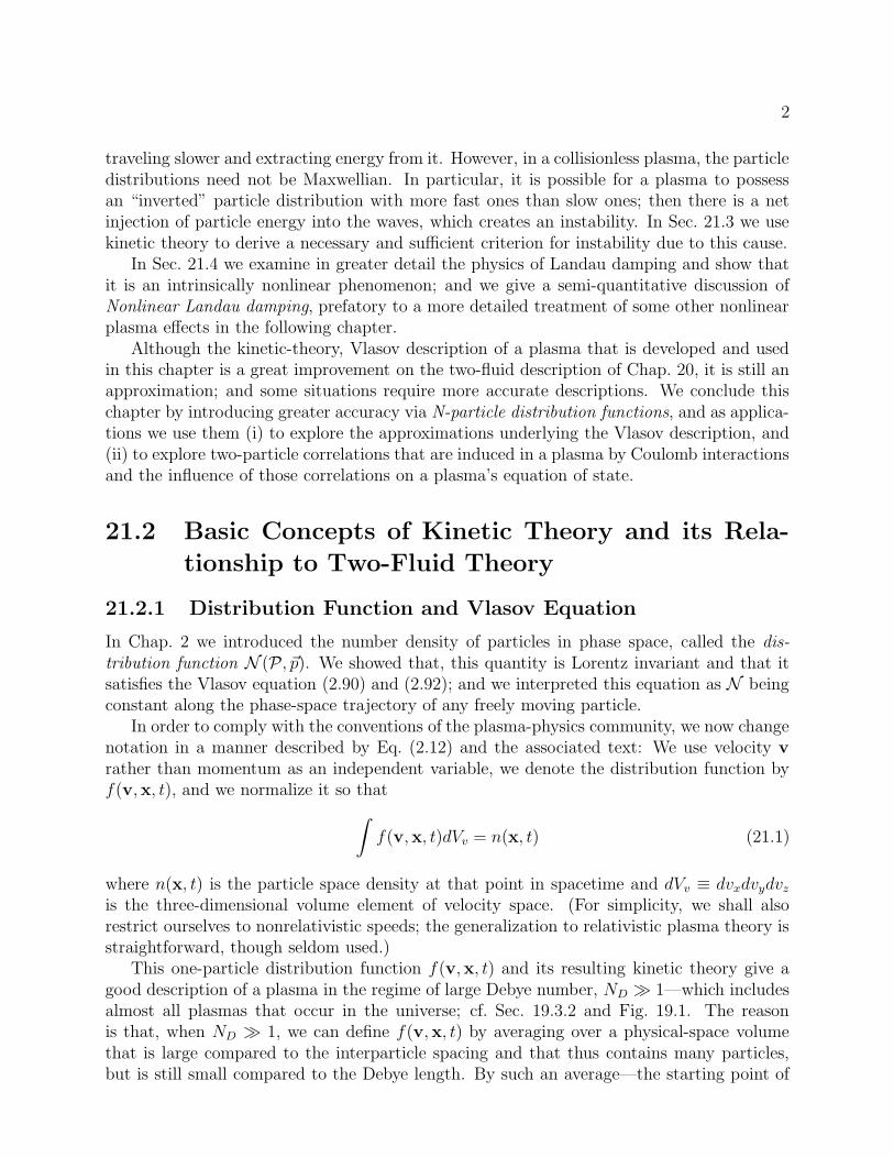
variables. In particular, any function of the integrals of motion alone that is independentof the remaining initial coordinates will satisfy the Vlasov equation (21.5). This is Jeans’Theorem. In words, functions of constants of the motion take constant values along actualdynamical trajectories in phase space and therefore satisfy the Vlasov equation.

Of course, a situation may be so complex that no integrals of the particles’ equation ofmotion can be found, in which case, Jeans’ theorem is useless. Alternatively, there maybe integrals but the initial conditions may be sufficiently complex that extra variables arerequired to determine fs. However, it turns out that in a wide variety of applications,particularly those with symmetries such as time independence ∂fs/∂t = 0, simple functionsof simple integrals suffice to describe a plasma’s distribution functions.

We have already met and used a variant of Jeans’ theorem in our analysis of statisticalequilibrium in Sec. 3.4. There the statistical mechanics distribution function ρ was found todepend only on the integrals of the motion.

We have also, unknowingly, used Jeans’ theorem in our discussion of Debye screening ina plasma (Sec. 19.3.1). To understand this, let us suppose that we have a single isolatedpositive charge at rest in a stationary plasma (∂fs/∂t = 0), and we want to know the electrondistribution function in its vicinity. Let us further suppose that the electron distributionat large distances from the charge is known to be Maxwellian with temperature T , i.e.fe(v,x, t) ∝ exp(− 1

2mev

2/kBT ). Now, the electrons have an energy integral, E = 12mev

2 −eΦ, where Φ is the electrostatic potential. As Φ becomes constant at large distance from thecharge, we can therefore write fe ∝ exp(−E/kBT ) at large distance. However, the particlesnear the charge must have traveled there from large distance and so must have this samedistribution function. Therefore, close to the charge,

fe ∝ e−E/kBT = e−[(mev2/2−eΦ)/kBT ] , (21.12)

and the electron density is obtained by integration over velocity

ne =

∫

fe dVv ∝ e(eΦ/kBT ) . (21.13)

This is just the Boltzmann distribution that we asserted to be appropriate in Sec. 19.3.1.

****************************

EXERCISES

Exercise 21.1 Derivation: Two-fluid Equation of MotionDerive the two-fluid equation of motion (21.11) by multiplying the Vlasov equation (21.5)by v and integrating over velocity space.

Exercise 21.2 Example: Positivity of Distribution FunctionThe one-particle distribution function f(x,v, t) ought not to become negative if it is toremain physical. Show that this is guaranteed if it initially is everywhere nonnegative andit evolves by the collisionless Vlasov equation.

****************************

7

21.3 Electrostatic Waves in an Unmagnetized Plasma:

Landau Damping

21.3.1 Formal Dispersion Relation

As our principal application of the kinetic theory of plasmas, we shall explore its predictionsfor the dispersion relations, stability, and damping of longitudinal, electrostatic waves in anunmagnetized plasma—Langmuir waves and ion acoustic waves. When studying these wavesin Sec. 20.3 using two-fluid theory, we alluded time and again to properties of the waves thatcould not be derived by fluid techniques. Our goal, now, is to elucidate those properties usingkinetic theory. As we shall see, their origin lies in the plasma’s velocity-space dynamics.

Consider an electrostatic wave propagating in the z direction. Such a wave is one dimen-sional in that the electric field points in the z direction, E = Eez, and varies as ei(kz−ωt) soit depends only on z and not on x or y; the distribution function similarly varies as ei(kz−ωt)

and is independent of x, y; and the Vlasov, Maxwell, and Lorentz force equations produceno coupling of particle velocities vx, vy into the z direction. This suggests the introductionof one-dimensional distribution functions, obtained by integration over vx and vy:

Fs(v, z, t) ≡∫

fs(vx, vy, v = vz, z, t)dvxdvy . (21.14)

Here and throughout we suppress the subscript z on vz.Restricting ourselves to weak waves so nonlinearities can be neglected, we linearize the

one-dimensional distribution functions:

Fs(v, z, t) ' Fs0(v) + Fs1(v, z, t) . (21.15)

Here Fs0(v) is the distribution function of the unperturbed particles (s = e for electrons ands = p for protons) in the absence of the wave and Fs1 is the perturbation induced by andlinearly proportional to the electric field E. The evolution of Fs1 is governed by the linearapproximation to the Vlasov equation (21.5):

∂Fs1

∂t+ v

∂Fs1

∂z+

qsE

ms

dFs0

dv. (21.16)

We seek a monochromatic, plane-wave solution to this Vlasov equation, so ∂/∂t → −iωand ∂/∂z → ik in Eq. (21.16). Solving the resulting equation for Fs1, we obtain an equationfor Fs1 in terms of E:

Fs1 =−iqs

ms(ω − kv)

dFs0

dvE . (21.17)

This equation implies that the charge density associated with the wave is related to theelectric field by

ρe =∑

s

qs

∫ +∞

−∞

Fs1dv =

(

∑

s

−iq2s

ms

∫ +∞

−∞

F ′s0 dv

ω − kv

)

E , (21.18)

8

where the prime denotes a derivative with respect to v: F ′s0 = dFs0/dv.

A quick route from here to the waves’ dispersion relation is to insert this charge densityinto Poisson’s equation ∇ · E = ikE = ρe/ε0 and note that both sides are proportional toE, so a solution is possible only if

1 +∑

s

q2s

msε0k

∫ +∞

−∞

F ′s0 dv

ω − kv= 0 . (21.19)

An alternative route, which makes contact with the general analysis of waves in a dielectricmedium (Sec. 20.2), is developed in Ex. 21.3 below. This route reveals that the dispersionrelation is given by the vanishing of the zz component of the dielectric tensor, which wedenoted ε3 in Chap. 20 [cf. Eq. (20.49)], and it shows that ε3 is given by expression (21.19):

ε3(ω, k) = 1 +∑

s

q2s

msε0k

∫ +∞

−∞

F ′s0 dv

ω − kv= 0 . (21.20)

Since ε3 = εzz is the only component of the dielectric tensor that we shall meet in thischapter, we shall simplify notation henceforth by omitting the subscript 3.

The form of the dispersion relation (21.20) suggests that we combine the unperturbedelectron and proton distribution functions Fe0(v) and Fp0(v) to produce a single, unifieddistribution function

F (v) = Fe0(v) +me

mpFp0(v) , (21.21)

in terms of which Eq. (21.20) takes the form

ε(ω, k) = 1 +e2

meε0k

∫ +∞

−∞

F ′ dv

ω − kv= 0 (21.22)

Note that each proton is weighted less heavily than each electron by a factor me/mp =1/1860 in the unified distribution function (21.21) and the dispersion relation (21.22). This isdue to the protons’ greater inertia and corresponding weaker response to an applied electricfield, and it causes the protons to be of no importance in Langmuir waves (Sec. 21.3.5 below).However, in ion-acoustic waves (Sec. 21.3.6), the protons can play an important role becauselarge numbers of them may move with thermal speeds that are close to the waves’ phasevelocity and thereby can interact resonantly with the waves.

21.3.2 Two-Stream Instability

As a first application of the general dispersion relation (21.22), we use it to rederive thedispersion relation (20.76) associated with the cold-plasma two-stream instability of Sec. 20.7.

We begin by performing an integration by parts on the general dispersion relation (21.22),obtaining:

e2

meε0

∫ +∞

−∞

Fdv

(ω − kv)2= 1 . (21.23)

We then presume, as in Sec. 20.7, that the fluid consists of two or more streams of coldparticles (protons or electrons) moving in the z direction with different fluid speeds u1, u2,

9

. . ., so F (v) = n1δ(v − u1) + n2δ(v − u2) + . . .. Here nj is the number density of particlesin stream j if the particles are electrons, and me/mp times the number density if they areprotons. Inserting this F (v) into Eq. (21.22) and noting that nje

2/meε0 is the squaredplasma frequency ω2

pj of stream j, we obtain the dispersion relation

ω2p1

(ω − ku1)2+

ω2p2

(ω − ku2)2+ . . . = 1 , (21.24)

which is identical to the dispersion relation Eq. (20.76) used in our analysis of the two-streaminstability.

Clearly the general dispersion relation (21.23) [or equally well (21.22)] provides us with atool for exploring how the two-stream instability is influenced by a warming of the plasma,i.e. by a spread of particle velocities around the mean, fluid velocity of each stream. Weshall explore this in Sec. 21.4 below.

21.3.3 The Landau Contour

The general dispersion relation (21.22) has a troubling feature: for real ω and k its integrandbecomes singular at v = ω/k = (the waves’ phase velocity) unless dF/dv vanishes there,which is generically unlikely. This tells us that if, as we shall assume, k is real, then ωcannot be real, except, perhaps, for a non-generic mode whose phase velocity happens tocoincide with a velocity for which dF/dv = 0.

With ω/k complex, we must face the possibility of some subtlety in how the integral overv in the dispersion relation (21.22) is performed—the possibility that we may have to makev complex in the integral and follow some special route in the complex velocity plane fromv = −∞ to v = +∞. Indeed, there is such a subtlety, as Lev Landau has shown.2 Oursimple derivation of the dispersion relation, above, cannot reveal this subtlety—and, indeed,is suspicious, since in going from Eq. (21.16) to (21.17) our derivation entailed dividing byω − kv which vanishes when v = ω/k, and dividing by zero is always a suspicious practice.Faced by this conundrum, Landau developed a more sophisticated derivation of the dispersionrelation, one based on posing generic initial data for electrostatic waves, then evolving thosedata forward in time and identifying the plasma’s electrostatic modes by their late-timesinusoidal behaviors, and finally reading off the dispersion relation for the modes from theequations for the late-time evolution. We shall sketch a variant of this analysis:

For simplicity, from the outset we restrict ourselves to plane waves propagating in the zdirection with some fixed, real wave number k, so the linearized one-dimensional distributionfunction and the electric field have the forms

Fs(v, z, t) = Fs0(v) + Fs1(v, t)eikz , E(t)eikz . (21.25)

At t = 0 we pose initial data Fs1(v, 0) for the electron and proton velocity distributions;these data determine the initial electric field E(0) via Poisson’s equation. We presume thatthese initial distributions [and also the unperturbed plasma’s velocity distribution Fs0(v)] areanalytic functions of velocity v, but aside from this constraint the Fs1(v, 0) are generic. (A

2Landau, L. D. 1946. J. Phys. USSR, 10, 25.

10

ωr

ωi

σ

ω

ωω

ω1

2

3

4

Fig. 21.1: Contour of integration for evaluating E(t) [Eq. (21.26)] as a sum over residues of theintegrand’s poles—the modes of the plasma.

Maxwellian distribution is analytic, and most any physically reasonable initial distributioncan be well approximated by an analytic function.)

We then evolve these initial data forward in time. The ideal tool for such evolution isthe Laplace transform, and not the Fourier transform. The power of the Laplace transformis much appreciated by engineers, and under-appreciated by many physicists. Those readerswho are not intimately familiar with evolution via Laplace transforms should work carefullythrough Ex. 21.4. That exercise uses Laplace transforms, followed by conversion of the finalanswer into Fourier language, to derive the following formula for the time-evolving electricfield in terms of the initial velocity distributions Fs1(v, 0):

E(t) = −∫ iσ+∞

iσ−∞

e−iωt

ε(ω, k)

[

∑

s

qs

2πε0k

∫ +∞

−∞

Fs1(v, 0)

ω − kvdv

]

dω . (21.26)

Here the integral in frequency space is along the solid horizontal line at the top of Fig. 21.1,with the imaginary part of ω held fixed at ωi = σ and the real part ωr varying from −∞to +∞. The Laplace techniques used to derive this formula are carefully designed to avoidany divergences and any division by zero. This careful design leads to the requirement thatthe height σ of the integration line above the real frequency axis be larger than the e-foldingrate =(ω) of the plasma’s most rapidly growing mode (or, if none grow, still larger than zeroand thus larger than the e-folding rate of the most slowly decaying mode):

σ > maxn

=(ωn) , and σ > 0 , (21.27)

where n = 1, 2, . . . labels the modes and ωn is the complex frequency of mode n.Equation (21.26) also entails a velocity integral. In the Laplace-based analysis that leads

to this formula, there is never any question about the nature of the velocity v: it is alwaysreal, so the integral is over real v running from −∞ to +∞. However, because all thefrequencies ω appearing in Eq. (21.26) have ωi = σ > 0, there is no possibility in the velocityintegral of any divergence of the integrand.

11

In Eq. (21.26) for the evolving field, ε(ω, k) is the same dielectric function as we deducedin our previous analysis (Sec. 21.3.1):

ε(ω, k) = 1 +e2

meε0k

∫ +∞

−∞

F ′ dv

ω − kv. (21.28)

However, here by contrast with there our derivation has dictated unequivocally how to handlethe v integration—the same way as in Eq. (21.26): v is strictly real and the only frequenciesappearing in the evolution equations have ωi = σ > 0, so the v integral running along thereal velocity axis passes under the integrand’s pole at v = ω/k as shown in Fig. 21.2(a).

To read off the modal frequencies from the evolving field E(t) at times t > 0, we usetechniques from complex-variable theory. It can be shown that, because (by hypothesis)Fs1(v, 0) and Fs0(v) are analytic functions of v, the integrand of the ω integral in Eq. (21.26)is meromorphic—i.e., when the integrand is analytically continued throughout the complexfrequency plane, its only singularities are poles. This permits us to evaluate the frequency in-tegral, at times t > 0, by closing the integration contour in the lower-half frequency plane asshown by the dashed curve in Fig. 21.1. Because of the exponential factor e−iωt, the contribu-tion from the dashed part of the contour vanishes, which means that the integral around thecontour is equal to E(t) (the contribution from the solid horizontal part). Complex-variabletheory tells us that this integral is given by a sum over the residues Rn of the integrand atthe poles (labeled n = 1, 2, . . .):

E(t) = 2πi∑

n

Rn =∑

n

Ane−iωnt . (21.29)

Here ωn is the frequency at pole n and An is 2πiRn with its time dependence e−iωnt factoredout. It is evident, then, that each pole of the analytically continued integrand of Eq. (21.26)corresponds to a mode of the plasma and the pole’s complex frequency is the mode’s frequency.

Now, for very special choices of the initial data Fs1(v, 0), there may be poles in thesquare-bracket term in Eq. (21.26), but for generic initial data there will be none, and theonly poles will be the zeroes of ε(ω, k). Therefore, generically, the modes’ frequencies arethe zeroes of ε(ω, k)—when that function (which was originally defined only along the lineωi = σ) has been analytically extended throughout the complex frequency plane.

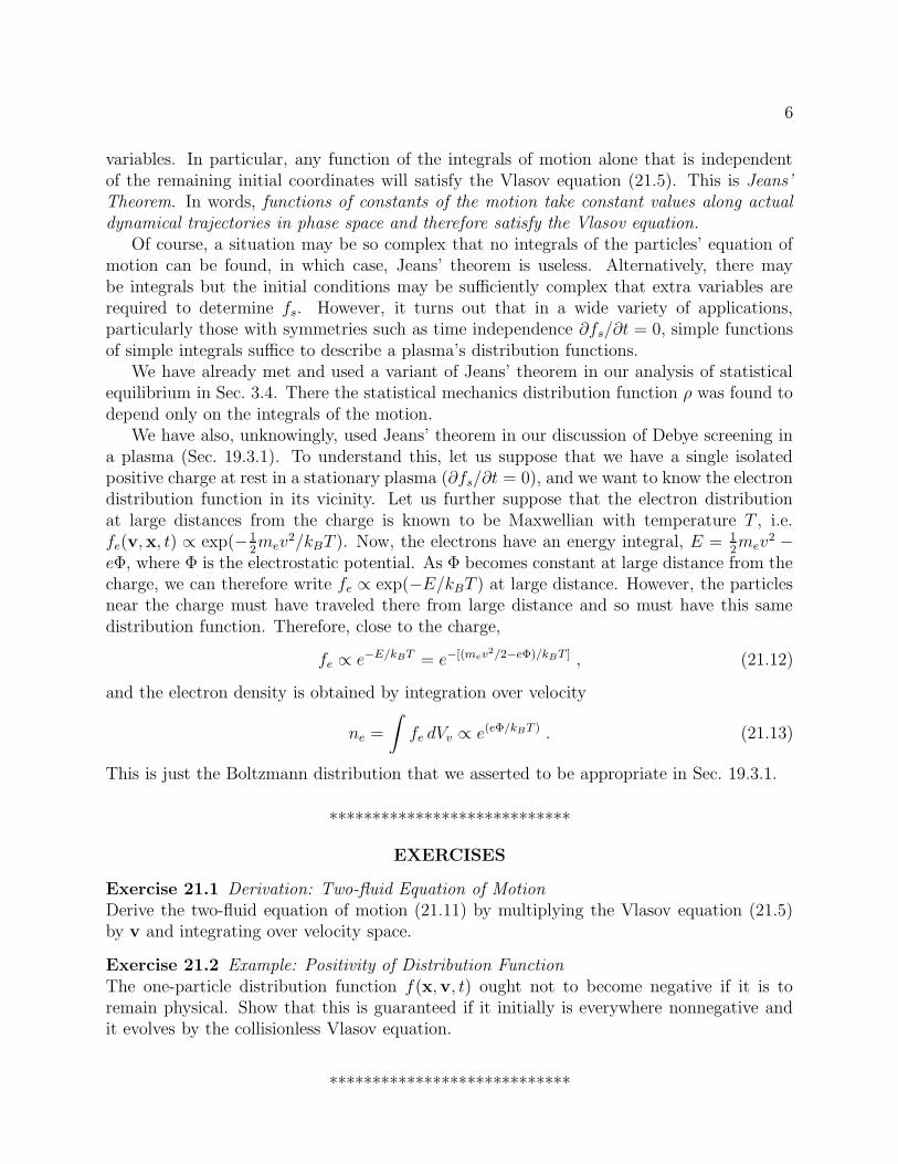
So how do we compute the analytically extended dielectric function ε(ω, k)? Imagineholding k fixed and real, and exploring the (complex) value of ε, thought of as a functionof ω/k, by moving around the complex ω/k plane (same as complex velocity plane). Inparticular, imagine computing ε from Eq. (21.28) at one point after another along the arrowedpath shown in Fig. 21.2. This path begins at an initial location ω/k where ωi/k = σ/k > 0and travels downward to some other location below the real axis. At the starting point, thediscussion following Eq. (21.28) tells us how to handle the velocity integral: just integrate valong the real axis. As ω/k is moved continuously (with k held fixed), ε(ω, k) being analyticmust vary continuously. If, when ω/k crosses the real velocity axis, the integration contourin Eq. (21.28) were to remain on the velocity axis, then the contour would jump over theintegral’s moving pole v = ω/k, and there would be a discontinuous jump of the functionε(ω, k) at the moment of crossing, which is not possible. To avoid such a discontinous jump,it is necessary that the contour of integration be kept below the pole, v = ω/k, as that pole

12

vi

vr

vi

vr

vi

vr

(a) (b) (c)

L L

ω/k

ω/k

ω/k

σ/k

Fig. 21.2: Derivation of the Landau contour L: The dielectric function ε(ω, k) is originally defined,in Eqs. (21.26) and (21.28), solely for ωi/k = σ/k > 0, the point in diagram (a). Since ε(ω, k) mustbe an analytic function of ω at fixed k and thus must vary continuously as ω is continuously changed,the dashed contour of integration in Eq. (21.28) must be kept always below the pole v = ω/k, asshown in (b) and (c).

moves into the lower half velocity plane; cf. Fig. 21.2(b,c). The rule that the integrationcontour must always pass beneath the pole v = ω/k as shown in Fig. 21.2 is called theLandau prescription; the contour is called the Landau contour and is denoted L; and ourfinal formula for the dielectric function (and for its vanishing at the modal frequencies—thedispersion relation) is

ε(ω, k) = 1 +e2

meε0k

∫

L

F ′dv

ω − kv= 0 . (21.30)

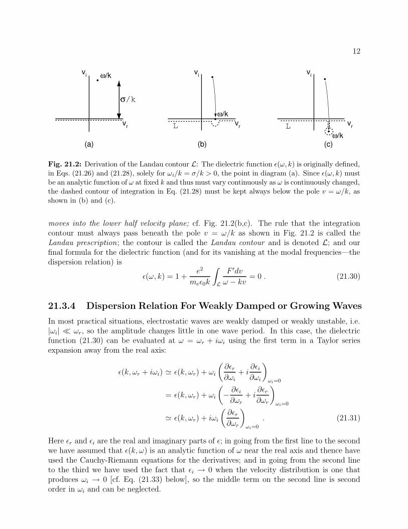
21.3.4 Dispersion Relation For Weakly Damped or Growing Waves

In most practical situations, electrostatic waves are weakly damped or weakly unstable, i.e.|ωi| � ωr, so the amplitude changes little in one wave period. In this case, the dielectricfunction (21.30) can be evaluated at ω = ωr + iωi using the first term in a Taylor seriesexpansion away from the real axis:

ε(k, ωr + iωi) ' ε(k, ωr) + ωi

(

∂εr

∂ωi+ i

∂εi

∂ωi

)

ωi=0

= ε(k, ωr) + ωi

(

− ∂εi

∂ωr+ i

∂εr

∂ωr

)

ωi=0

' ε(k, ωr) + iωi

(

∂εr

∂ωr

)

ωi=0

. (21.31)

Here εr and εi are the real and imaginary parts of ε; in going from the first line to the secondwe have assumed that ε(k, ω) is an analytic function of ω near the real axis and thence haveused the Cauchy-Riemann equations for the derivatives; and in going from the second lineto the third we have used the fact that εi → 0 when the velocity distribution is one thatproduces ωi → 0 [cf. Eq. (21.33) below], so the middle term on the second line is secondorder in ωi and can be neglected.

13

Equation (21.31) expresses the dielectric function slightly away from the real axis in termsof its value and derivative on and along the real axis. The on-axis value can be computed bybreaking the Landau contour depicted in Fig. 21.2(b) into three pieces: two lines from ±∞to a small distance δ from the pole, plus a semicircle of radius δ around the pole, and bythen taking the limit δ → 0. The first two terms (the two straight lines) together producethe Cauchy principle value of the integral (denoted

∫

Pbelow), and the third produces 2πi

times half the residue of the pole at v = ωr/k:

ε(k, ωr) = 1 − e2

meε0k2

[∫

P

F ′ dv

v − ωr/kdv + iπF ′(v = ωr/k)

]

. (21.32)

Inserting this equation and its derivative with respect to ωr into Eq. (21.31), and setting theresult to zero, we obtain

ε(k, ωr+iωi) ' 1− e2

meε0k2

[∫

P

F ′ dv

v − ωr/k+ iπF ′(ωr/k) + iωi

∂

∂ωr

∫

P

F ′ dv

v − ωr/k

]

= 0 . (21.33)

This is the dispersion relation in the limit |ωi| � ωr.Notice that the vanishing of εr determines the real part of the frequency

1 − e2

meε0k2

∫

P

F ′

v − ωr/kdv = 0 , (21.34)

and the vanishing of εi determines the imaginary part

ωi =πF ′(ωr/k)

∂∂ωr

∫

PF ′

v−ωr/kdv

. (21.35)

Notice, further, that the sign of ωi is influenced by the sign of F ′ = dF/dv at v = ωr/k =Vφ = (the waves’ phase velocity). As we shall see, this has a simple physical origin andimportant physical consequences.

21.3.5 Langmuir Waves and their Landau Damping

We shall now apply the dispersion relation (21.33) to Langmuir waves in a thermalizedplasma. Langmuir waves typically move so fast that the slow ions cannot interact with them,so their dispersion relation is influenced significantly only by the electrons. We therefore shallignore the ions and include only the electrons in F (v). We obtain F (v) by integrating outvy and vz in the 3-dimensional Maxwellian velocity distribution (2.39); the result is

F = n

(

me

2πkBT

)1/2

e−(mev2/2kBT ) , (21.36)

where T is the electron temperature.Now, as we saw in Eq. (21.35), |ωi| ∝ |F ′(v = ωr/k)|. Physically, this proportionality

arises from the manner in which electrons surf on the waves: Those electrons moving slightlyfaster than the waves’ phase velocity Vφ = ωr/k lose energy to the waves, while those

14

moving slightly slower extract energy from the waves; so the bigger the disparity betweenthe number of slightly faster electrons and the number of slightly slower electrons, i.e. thebigger F ′(ωr/k), the larger will be the damping or growth of wave energy, i.e. the larger willbe |ωi|. It will turn out, quantitatively, that, if the waves’ phase velocity ωr/k is anywherenear the steepest point on the side of the electron velocity distribution, i.e. if ωr/k is of orderthe electron thermal velocity

√

kBT/me, then the waves will be strong damped, ωi ∼ −ωr.Since our dispersion relation (21.36) is valid only when the waves are weakly damped, wemust restrict ourseves to waves with ωr/k �

√

kBT/me (a physically allowed regime) or to

ωr/k �√

kBT/me (a regime that does not occur in Langmuir waves; cf. Fig. 20.1).

Requiring, then, that ωr/k �√

kBT/me and noting that the integral in Eq. (21.33) gets

its dominant contribution from velocities v .√

kBT/me, we can expand 1/(v−ωr/k) in theintegrand as a power series in vk/ωr, obtaining

∫

P

F ′ dv

v − ωr/k=

∫ ∞

−∞

dvF ′

[

k

ωr+

k2v

ω2r

+k3v2

ω3r

+k4v3

ω4r

+ . . .

]

=nk2

ω2r

+3n〈v2〉k4

ω4r

+ . . .

=nk2

ω2r

(

1 +3kBTk2

meω2r

+ . . .

)

' nk2

ω2r

(

1 + 3k2λ2D

ω2p

ω2r

)

. (21.37)

Substituting Eqs. (21.36) and (21.37) into Eq. (21.33), evaluating the real and imaginaryparts, and noting that ωr/k �

√

kBT/me ≡ ωpλD implies kλD � 1 and ωr ' ωp, we obtain

ωr = ωp(1 + 3k2λ2D)1/2

ωi = −(π

8

)1/2 ωp

k3λ3D

exp

(

− 1

2k2λ2D

− 3

2

)

. (21.38)

The real part of this dispersion relation, ωr = ωp

√

1 + 3k2λ2D, reproduces the Bohm-

Gross result that we derived from fluid theory in Sec. 20.3.4 and plotted in Fig. 20.1. Theimaginary part reveals the damping of these Langmuir waves by surfing electrons—so-calledLandau damping. The fluid theory could not predict this Landau damping, because it is aresult of the internal dynamics in velocity space, of which the fluid theory is obvlivious.

Notice that, as the waves’ wavelength is decreased, i.e. as k increases, the waves’ phasevelocity decreases toward the electron thermal velocity and the damping becomes stronger,as is expected from our discussion of the number of electrons that can surf on the waves. Inthe limit k → 1/λD (where our dispersion relation has broken down and so is only an order-of-magnitude guide), the dispersion relation predicts that ωr/k ∼

√kBT and ωi/ωr ∼ 1/10.

In the opposite regime of large wavelength kλD � 1 (where our dispersion relation shouldbe quite accurate), the Landau damping is very weak—so weak that ωi decreases to zerowith increasing k faster than any power of k.

15

F

F

e

p

F

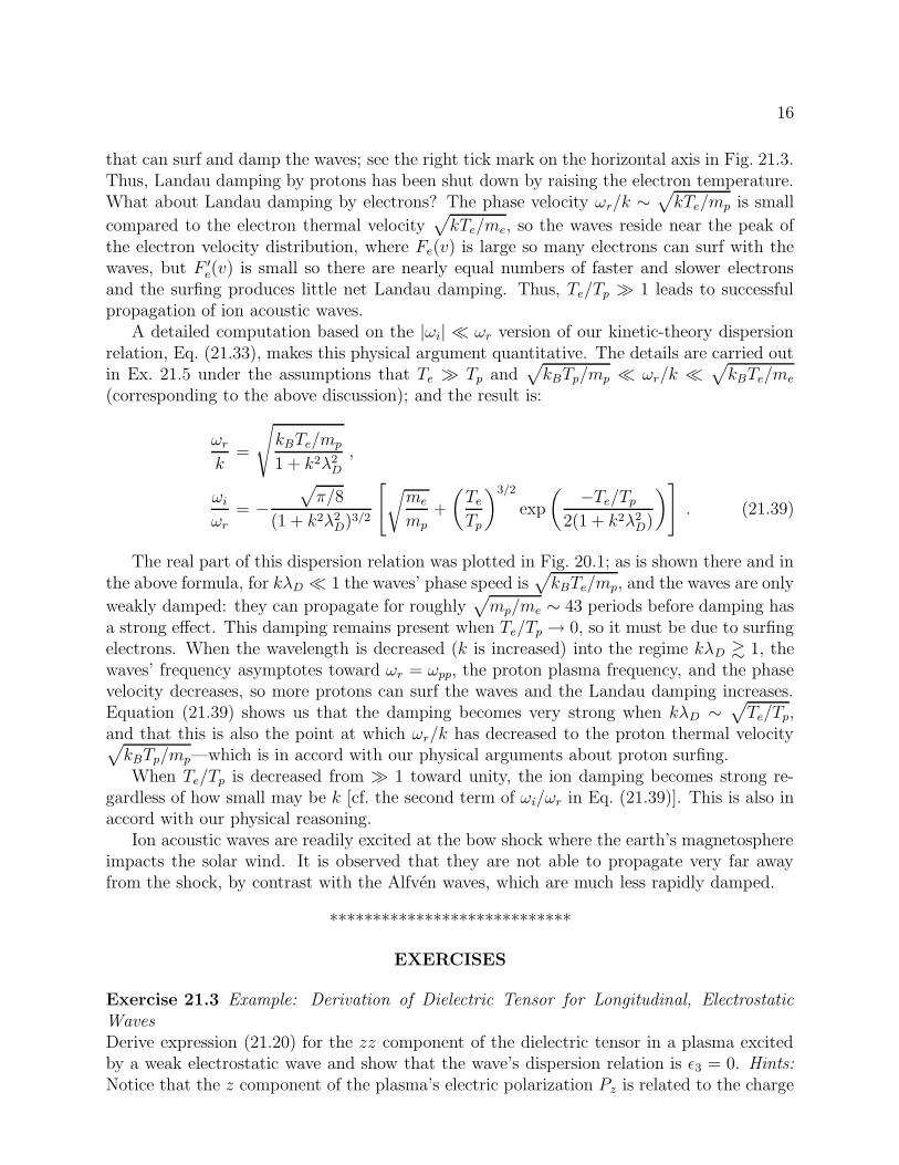
Fig. 21.3: Electron and ion contributions to the net distribution function F (v)in a thermalizedplasma. When Te ∼ Tp, the phase speed of ion acoustic waves is near the left tick mark on thehorizontal axis—a speed at which surfing protons have a maximal ability to Landau-damp thewaves, and the waves are strongly damped. When Te � Tp, the phase speed is near the right tickmark—far out on the tail of the proton velocity distribution so few protons can surf and damp thewaves, and near the peak of the electron distribution so the number of electrons moving slightlyslower than the waves is nearly the same as the number moving slightly faster and there is littlenet damping by the electrons. In this case the waves can propagate.

21.3.6 Ion Acoustic Waves and Conditions for their Landau Damp-

ing to be Weak

As we saw in Sec. 20.3.4, ion acoustic waves are the analog of ordinary sound waves in a fluid:They occur at low frequencies where the mean (fluid) electron velocity is very nearly locked tothe mean (fluid) proton velocity so the electric polarization is small; the restoring force is dueto thermal pressure and not to the electrostatic field; and the inertia is provided by the heavyprotons. It was asserted in Sec. 20.3.4 that to avoid these waves being strongly damped, theelectron temperature must be much higher than the proton temperature, Te � Tp. We cannow understand this in terms of particle surfing and Landau damping:

Suppose that the electrons and protons have Maxwellian velocity distributions but possi-bly with different temperatures. Because of their far greater inertia, the protons will have afar smaller mean thermal speed than the electrons, so the net one-dimensional distributionfunction F (v) = Fe(v) + (me/mp)Fp(v) [Eq. (21.21)] that appears in the kinetic-theory dis-persion relation has the form shown in Fig. 21.3. Now, if Te ∼ Tp, then the contributions ofthe electron pressure and proton pressure to the waves’ restoring force will be comparable,and the waves’ phase velocity will therefore be ωr/k ∼

√

k(Te + Tp)/mp ∼√

kTp/mp, whichis the speed at which the proton contribution to F (v) has its steepest slope (see the lefttick mark on the horizontal axis in Fig. 21.3), so |F ′(v = ωr/k)| is large. This means therewill be large numbers of protons that can surf on the waves and a large disparity betweenthe number moving slightly slower than the waves (which extract energy from the waves)and the number moving slightly faster (which give energy to the waves). The result will bestrong Landau damping by the protons.

This strong Landau damping is avoided if Te � Tp. Then the waves’ phase velocity willbe ωr/k ∼

√

kTe/mp which is large compared to the proton thermal velocity√

kTp/mp andso is way out on the tail of the proton velocity distribution where there are very few protons

16

that can surf and damp the waves; see the right tick mark on the horizontal axis in Fig. 21.3.Thus, Landau damping by protons has been shut down by raising the electron temperature.What about Landau damping by electrons? The phase velocity ωr/k ∼

√

kTe/mp is small

compared to the electron thermal velocity√

kTe/me, so the waves reside near the peak ofthe electron velocity distribution, where Fe(v) is large so many electrons can surf with thewaves, but F ′

e(v) is small so there are nearly equal numbers of faster and slower electronsand the surfing produces little net Landau damping. Thus, Te/Tp � 1 leads to successfulpropagation of ion acoustic waves.

A detailed computation based on the |ωi| � ωr version of our kinetic-theory dispersionrelation, Eq. (21.33), makes this physical argument quantitative. The details are carried outin Ex. 21.5 under the assumptions that Te � Tp and

√

kBTp/mp � ωr/k �√

kBTe/me

(corresponding to the above discussion); and the result is:

ωr

k=

√

kBTe/mp

1 + k2λ2D

,

ωi

ωr= −

√

π/8

(1 + k2λ2D)3/2

[

√

me

mp+

(

Te

Tp

)3/2

exp

( −Te/Tp

2(1 + k2λ2D)

)

]

. (21.39)

The real part of this dispersion relation was plotted in Fig. 20.1; as is shown there and inthe above formula, for kλD � 1 the waves’ phase speed is

√

kBTe/mp, and the waves are only

weakly damped: they can propagate for roughly√

mp/me ∼ 43 periods before damping hasa strong effect. This damping remains present when Te/Tp → 0, so it must be due to surfingelectrons. When the wavelength is decreased (k is increased) into the regime kλD & 1, thewaves’ frequency asymptotes toward ωr = ωpp, the proton plasma frequency, and the phasevelocity decreases, so more protons can surf the waves and the Landau damping increases.Equation (21.39) shows us that the damping becomes very strong when kλD ∼

√

Te/Tp,and that this is also the point at which ωr/k has decreased to the proton thermal velocity√

kBTp/mp—which is in accord with our physical arguments about proton surfing.When Te/Tp is decreased from � 1 toward unity, the ion damping becomes strong re-

gardless of how small may be k [cf. the second term of ωi/ωr in Eq. (21.39)]. This is also inaccord with our physical reasoning.

Ion acoustic waves are readily excited at the bow shock where the earth’s magnetosphereimpacts the solar wind. It is observed that they are not able to propagate very far awayfrom the shock, by contrast with the Alfven waves, which are much less rapidly damped.

****************************

EXERCISES

Exercise 21.3 Example: Derivation of Dielectric Tensor for Longitudinal, ElectrostaticWavesDerive expression (21.20) for the zz component of the dielectric tensor in a plasma excitedby a weak electrostatic wave and show that the wave’s dispersion relation is ε3 = 0. Hints:Notice that the z component of the plasma’s electric polarization Pz is related to the charge

17

density by ∇ · P = ikPz = −ρe [Eq. (20.1)]; combine this with Eq. (21.18) to get a linearrelationship between Pz and Ez = E; argue that the only nonzero component of the plasma’selectric susceptibility is χzz and deduce its value by comparing the above result with Eq.(20.3); then construct the dielectric tensor εij from Eq. (20.5) and the algebratized waveoperator Lij from Eq. (20.9), and deduce that the dispersion relation det||Lij|| = 0 takes theform εzz ≡ ε3 = 0, where ε3 is given by Eq. (21.20).

Exercise 21.4 Example: Landau Contour Deduced Using Laplace TransformsUse Laplace-transform techniques to derive Eqs. (21.26)–(21.28) for the time-evolving elec-tric field of electrostatic waves with fixed wave number k and initial velocity perturbationsFs1(v, 0). A sketch of the solution follows.

(a) When the initial data are evolved forward in time, they produce F1(v, t) and E(t).Construct the Laplace transforms of these evolving quantities:3

F1(v, p) =

∫ ∞

0

dte−ptF1(v, t) , E(p) =

∫ ∞

0

dte−ptE(t) . (21.40)

To ensure that the time integral is convergent, insist that <(p) be greater than p0 ≡maxn =(ωn) ≡ (the e-folding rate of the most strongly growing mode—or, if nonegrow, then the most weakly damped mode). This is an essential step in the argumentleading to the Landau contour. Also, for simplicity of the subsequent analysis, insistthat <(p) > 0.

(b) By constructing the Laplace transform of the one-dimensional Vlasov equation (21.16)and integrating by parts the term involving ∂Fs1/∂t, obtain an equation for a linearcombination of Fs1(v, p) and E(p) in terms of the initial data Fs1(v, t = 0). By thencombining with the Laplace transform of Poisson’s equation, show that

E(p) =1

ε(ip, k)

∑

s

qs

kε0

∫ ∞

−∞

Fs1(v, 0)

ip − kvdv . (21.41)

Here ε(ip, k) is the dielectric function (21.22) evaluated for frequency ω = ip, withthe integral running along the real v axis, and [as we noted in part (a)] <(p) must begreater than p0, the largest ωi of any mode, and greater than 0. This situation for thedielectric function is the one depicted in Fig. 21.2(a).

(c) Laplace-transform theory tells us that the time-evolving electric field (with wave num-ber k) can be expressed in terms of its Laplace transform (21.41) by

E(t) =

∫ σ+i∞

σ−i∞

E(p)ept dp

2πi, (21.42)

where σ is any real number larger than p0 and larger than 0. Combine this equationwith expression (21.41) for E(p), and set p = iω. Thereby arrive at the desired result,Eq. (21.26).

3For useful insights into the Laplace transform, see, e.g., Sec. 4-2 of Mathews, J. and Walker, R. L., 1964,Mathematical Methods of Physics, New York: Benjamin.

18

Exercise 21.5 Derivation: Ion Acoustic Dispersion RelationConsider a plasma in which the electrons have a Maxwellian velocity distribution with tem-perature Te, the protons are Maxwellian with temperature Tp, and Tp � Te; and consider a

mode in this plasma for which√

kBTp/mp � ωr/k �√

kBTe/me (right tick mark in Fig.21.3). As was argued in the text, for such a mode it is reasonable to expect weak damping,|ωi| � ωr. Making approximations based on these “�” inequalities, show that the dispersionrelation (21.33) reduces to Eq. (21.39).

Exercise 21.6 Problem: Dispersion relations for a non-Maxwellian distribution function.Consider a plasma with cold protons [whose velocity distribution can be ignored in F (v)]and hot electrons with one dimensional distribution function of the form

F (v) =nv0

π(v20 + v2)

. (21.43)

(a) Derive the dielectric function ε(ω, k) for this plasma and use it to show that the dis-persion relation for Langmuir waves is

ω = ωpe − ikv0 . (21.44)

(b) Compute the dispersion relation for ion acoustic waves assuming that their phase speedsare much less than v0 but large compared to the cold protons’ thermal velocities (sothe contribution from proton surfing can be ignored). Your result should be

ω =kv0(me/mp)

1/2

[1 + (kv0/ωpe)2]1/2− ikv0(me/mp)

[1 + (kv0ωpe)2]2. (21.45)

****************************

21.4 Stability of Electrostatic Waves in Unmagnetized

Plasmas

Equation (21.35) implies that the sign of F ′ at resonance dictates the sign of the imaginarypart of ω. This raises the interesting possibility that distribution functions that increasewith velocity over some range of positive v might be unstable to the exponential growth ofelectrostatic waves. In fact, the criterion for instability turns out to be a little more complexthan this [as one might suspect from the fact that the sign of the denominator of Eq. (21.35)is non-obvious], and deriving it is an elegant exercise in complex variable theory.

Let us rewrite our dispersion relation (21.22) (again restricting our attention to realvalues of k) in the form

Z(ω/k) = k2 > 0 , (21.46)

where the complex function Z(ζ) is given by

Z(ζ) =e2

meε0

∫

L

F ′

v − ζdv . (21.47)

19

ζr

ζi

>

Zi

Zr>

<

∞ −∞ • P

Z Plane ζ Plane

C

C

ζP=vmin

Fig. 21.4: Mapping of the real axis in the complex ζ plane onto the Z plane; cf. Eq. (21.47). Thisis an example of a Nyquist diagram.

Now let us map the real axis in the complex ζ plane onto the Z plane (Fig. 21.4). Thepoints at (ζr = ±∞, ζi = 0) clearly map onto the origin and so the image of the real ζ axismust be a closed curve. Furthermore, by inspection, the region enclosed by the curve is theimage of the upper half plane. (The curve may cross itself, if ζ(Z) is multi-valued, but thiswill not affect our argument.) Now, there will be a growing mode (ζi > 0) if and only if thecurve crosses the positive real Z axis. Let us consider an upward crossing at some point Pas shown in Fig. 21.4 and denote by ζP the corresponding point on the real ζ axis. At thispoint, the imaginary part of Z vanishes, which implies immediately that F ′(v = ζP) = 0; cf.Eq. (21.35). Furthermore, as Zi is increasing at P (cf. Fig. 21.4), F ′′(v = ζP) > 0. Thus,for instability to the growth of Langmuir waves it is necessary that the one-dimensionaldistribution function have a minimum at some v = vmin ≡ ζP . This is not sufficient, as thereal part of Z(ζP) = Z(vmin) must also be positive.

Since vmin ≡ ζP is real, Zr(vmin) is the Cauchy principal value of the integral (21.47),which we can rewrite as follows using an integration by parts:

Zr(vmin) =

∫

P

F ′

v − ζdv =

∫

P

d[F (v) − F (vmin)]/dv

v − vmin

dv

=

∫

P

[F (v) − F (vmin)]

(v − vmin)2dv

+ limδ→0

[

F (vmin − δ) − F (vmin)

−δ− F (vmin + δ) − F (vmin)

δ

]

. (21.48)

The second, limit term vanishes since F ′(vmin) = 0, and in the first term we do not need theCauchy principal value because F is a minimum at vmin, so our requirement is that

Zr(vmin) =

∫ +∞

−∞

[F (v) − F (vmin)]

(v − vmin)2dv > 0 . (21.49)

Thus, a sufficient condition for instability is that there exist some velocity vmin at whichthe distribution function F (v) has a minimum, and that in addition the minimum be deep

20

enough that the integral (21.49) is positive. This is called the Penrose criterion for instabil-ity.4

****************************

EXERCISES

Exercise 21.7 Example: Penrose CriterionConsider an unmagnetized electron plasma with a one dimensional distribution function

F (v) ∝ {[(v − v0)2 + u2]−1 + [(v + v0)

2 + u2]−1} , (21.50)

where v0 and u are constants. Show that this distribution function possesses a minimum ifv0 > 3−1/2u, but the minimum is not deep enough to cause instability unless v0 > u.

****************************

21.5 Particle Trapping

We now return to the description of Landau damping. Our treatment so far has been essen-tially linear in the wave amplitude, or equivalently in the perturbation to the distributionfunction. What happens when the wave amplitude is not infinitesimally small?

Consider a single Langmuir wave mode as observed in a frame moving with the mode’sphase velocity. In this frame the electrostatic field oscillates spatially, E = E0 sin kz, buthas no time dependence. Figure 21.5 shows some phase-space orbits of electrons in thisoscillatory potential. The solid curves are orbits of particles that move fast enough to avoidbeing trapped in the potential wells at kz = 0, 2π, 4π, . . .. The dashed curves are orbits oftrapped particles. As seen in another frame, these trapped particles are surfing on the wave,with their velocities performing low-amplitude oscillations around the wave’s phase velocityω/k.

The equation of motion for an electron trapped in the minimum z = 0 has the form

z =−eE0 sin kz

me

' −ω2b z , (21.51)

where we have assumed small-amplitude oscillations and approximated sin kz ' kz, andwhere

ωb =

(

eEk

me

)1/2

(21.52)

is known as the bounce frequency. Since the potential well is actually anharmonic, thetrapped particles will mix in phase quite rapidly.

4Penrose, O. 1960, Phys. Fluids 3, 258.

21

z

v

Fig. 21.5: Phase-space Orbits for trapped (dashed lines) and untrapped (solid lines) electrons.

The growth or damping of the wave is characterized by a growth or damping of E0, andcorrespondingly by a net acceleration or deceleration of untrapped particles, when averagedover a wave cycle. It is this net feeding of energy into and out of the untrapped particlesthat causes the wave’s Landau damping or growth.

Now suppose that the amplitude E0 of this particular wave mode is changing on a timescale τ due to interactions with the electrons, or possibly (as we shall see in Chap. 22) due tointeractions with other waves propagating through the plasma. The potential well will thenchange on this same timescale and we expect that τ will also be a measure of the maximumlength of time a particle can be trapped in the potential well. These nonlinear, wave trappingeffects should only be important when the bounce period ∼ ω−1

b is short compared with τ ,i.e. when E � me/ekτ 2.

Electron trapping can cause particles to be bunched together at certain preferred phasesof a growing wave. This can have important consequences for the radiative properties ofthe plasma. Suppose, for example, that the plasma is magnetized. Then the electronsgyrate around the magnetic field and emit cyclotron radiation. If their gyrational phases arerandom then the total power that they radiate will be the sum of their individual particlepowers. However, if N electrons are localized at the same gyrational phase due to beingtrapped in a potential well of a wave, then, they will radiate like one giant electron witha charge Ne. As the radiated power is proportional to the square of the charge carried bythe radiating particle, the total power radiated by the bunched electrons will be N timesthe power radiated by the same number of unbunched electrons. Very large amplificationfactors are thereby possible both in the laboratory and in Nature, for example in the Jovianmagnetosphere.

This brief discussion suggests that there may be much more richness in plasma wavesthan is embodied in our dispersion relations with their simple linear growth and decay, evenwhen the wave amplitude is small enough that the particle motion is only slightly perturbedby its interaction with the wave. This motivates us to discuss more systematically nonlinearplasma physics, which is the topic of our next chapter.

****************************

22

z

Wp

W

W

We

-

+

eΦ

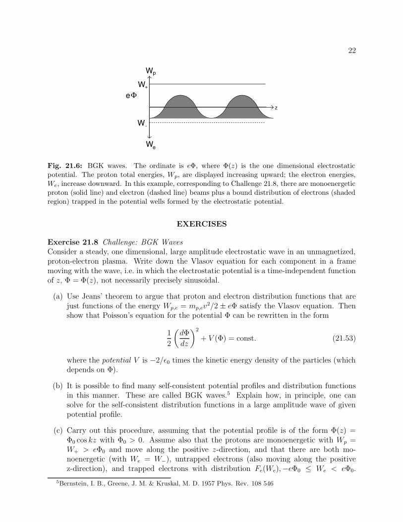
Fig. 21.6: BGK waves. The ordinate is eΦ, where Φ(z) is the one dimensional electrostaticpotential. The proton total energies, Wp, are displayed increasing upward; the electron energies,We, increase downward. In this example, corresponding to Challenge 21.8, there are monoenergeticproton (solid line) and electron (dashed line) beams plus a bound distribution of electrons (shadedregion) trapped in the potential wells formed by the electrostatic potential.

EXERCISES

Exercise 21.8 Challenge: BGK WavesConsider a steady, one dimensional, large amplitude electrostatic wave in an unmagnetized,proton-electron plasma. Write down the Vlasov equation for each component in a framemoving with the wave, i.e. in which the electrostatic potential is a time-independent functionof z, Φ = Φ(z), not necessarily precisely sinusoidal.

(a) Use Jeans’ theorem to argue that proton and electron distribution functions that arejust functions of the energy Wp,e = mp,ev

2/2 ± eΦ satisfy the Vlasov equation. Thenshow that Poisson’s equation for the potential Φ can be rewritten in the form

1

2

(

dΦ

dz

)2

+ V (Φ) = const. (21.53)

where the potential V is −2/ε0 times the kinetic energy density of the particles (whichdepends on Φ).

(b) It is possible to find many self-consistent potential profiles and distribution functionsin this manner. These are called BGK waves.5 Explain how, in principle, one cansolve for the self-consistent distribution functions in a large amplitude wave of givenpotential profile.

(c) Carry out this procedure, assuming that the potential profile is of the form Φ(z) =Φ0 cos kz with Φ0 > 0. Assume also that the protons are monoenergetic with Wp =W+ > eΦ0 and move along the positive z-direction, and that there are both mo-noenergetic (with We = W−), untrapped electrons (also moving along the positivez-direction), and trapped electrons with distribution Fe(We),−eΦ0 ≤ We < eΦ0.

5Bernstein, I. B., Greene, J. M. & Kruskal, M. D. 1957 Phys. Rev. 108 546

23

Show that the density of trapped electrons must vanish at the wave troughs (atz = (2n + 1)π/k; n = 0, 1, 2, 3 . . .). Let the proton density at the troughs be np0,and assume that there is no net current as well as no net charge density. Show thatthe total electron density can be written as

ne(z) =

[

me(W+ − eΦ0)

mp(W− + eΦ)

]1/2

np0 +

∫ eΦ0

−eΦ0

dWeFe(We)

[2me(We + eΦ)]1/2. (21.54)

(c) Use Poisson’s equation to show that

∫ ξ0

−ξ0

dWeFe(We)

[2me(We + ξ)]1/2=

ε0k2Φ

e2+ np0

[

(

W+ − ξ0

W+ − ξ

)1/2

−(

me(W+ − ξ0)

mp(W− + ξ)

)1/2]

,

(21.55)where eΦ0 = ξ0.

(d) Solve this integral equation for Fe(We). (Hint: it is of Abel type.)

(e) Exhibit some solutions graphically.

****************************

21.6 N Particle Distribution Function

Before turning to nonlinear phenomena in plasmas (the next chapter), let us digress brieflyand explore ways to study correlations between particles, of which our Vlasov formalism isoblivious.

The Vlasov formalism treats each particle as independent, migrating through phase spacein response to the local mean electromagnetic field and somehow unaffected by individualelectrostatic interactions with neighboring particles. As we discussed in chapter 19, thisis likely to be a good approximation in a collisionless plasma because of the influence ofscreening—except in the tiny “independent-particle” region of Fig. 19.1. However, we wouldlike to have some means of quantifying this and of deriving an improved formalism that takesinto account the correlations between individual particles.

One environment where this may be particularly relevant is the interior of the sun. Here,although the gas is fully ionized, the Debye number is not particularly large (i.e., one isnear the independent particle region of Fig. 19.1) and Coulomb corrections to the perfectgas equation of state may be responsible for measurable changes in the internal structure asderived, for example, using helioseismological analysis (cf. Sec. 15.2). In this application ourtask is simpler than in the general case because the gas will locally be in thermodynamicequilibrium at some temperature T . It turns out that the general case when the plasmadeparts significantly from thermal equilibrium is extremely hard to treat.

The one-particle distribution function that we use in the Vlasov formalism is the firstmember of a hierarchy of k-particle distribution functions, f (k)(x1,x2, . . . ,xk, v1,v2, . . . ,vk, t)

24

which equal the probability that particle 1 will be found in a volume of its phase space (whichwe shall denote by dx1dv1 ≡ dx1dx2dx3dvx1

dvx2dvx3

), and that particle 2 will be found involume dx2dv2 of its phase space, etc. Our probability interpretation of these distributionfunctions dictates for f (1) a different normalization than we use in the Vlasov formalism,f (1) = f/n where n is the number density of particles, and dictates that

∫

f (k)dx1dv1 · · ·dxkdvk = 1. (21.56)

It is useful to relate the distribution functions f (k) to the concepts of statistical mechanics,which we developed in Chap. 3. Suppose we have an ensemble of N -electron plasmas and letthe probability that a member of this ensemble is in a volume dNxdNv of 6N dimensionalphase space be F dNxdNv. (N is a very large number!) F satisfies the Liouville equation

∂F

∂t+

N∑

i=1

[

(vi · ∇i)F + (ai · ∇vi)F]

= 0 (21.57)

where ai is the electromagnetic acceleration of the i’th particle, and ∇i and ∇vi are gradients

with respect to the position and velocity of particle i. We can construct the k-particle“reduced” distribution function from the statistical-mechanics distribution function F byintegrating over all but k of the particles:

f (k)(x1,x2, . . . ,xk,v1,v2, . . . ,vk, t)

= Nk

∫

dxk+1 . . . dxNvk+1 . . . dvN F (x1, . . . ,xN ,v1, . . . ,vN) (21.58)

(Note: k is typically a very small number, by contrast with N ; below we shall only beconcerned with k = 1, 2, 3.) The reason for the prefactor N k in Eq. (21.58) is that whereasF referred to the probability of finding particle 1 in dx1dv1, particle 2 in dx2dv2 etc, thereduced distribution function describes the probability of finding any of the N identical,though distinguishable particles in dx1dv1 and so on. (As long as we are dealing withnon-degenerate plasmas we can count the electrons classically.) As N � k, the number ofpossible ways we can choose k particles for k locations in phase space is approximately N k.

For simplicity, suppose that the protons are immobile and form a uniform, neutraliz-ing background of charge so that we need only consider the electron distribution and itscorrelations. Let us further suppose that the forces associated with mean electromagneticfields produced by external charges and currents can be ignored. We can then restrict ourattention to direct electron-electron electrostatic interactions. The acceleration is then

ai =e

me

∑

j

∇iΦij , (21.59)

where Φij(xij) = −e/4πε0xij is the electrostatic potential between two electrons i, j andxij = |xi − xj|.

25

We can now derive the so-called BBGKY6 hierarchy of kinetic equations which relatethe k-particle distribution function to integrals over the k + 1 particle distribution func-tion. The first equation in this hierarchy is given by integrating Liouville’s Eq. (21.57) overdx2 . . . dxNdv2 . . . dvN . If we assume that the distribution function decreases to zero atlarge distances, then integrals of the type

∫

dxi∇ietildeF/∂xi vanish and the one particledistribution function evolves according to

∂f (1)

∂t+ (v1 · ∇)f (1) =

−eN

me

∫

dx2 . . . dxNdv2 . . . dvNΣj∇1Φ1j · ∇v1F

=−eN2

me

∫

dx2 . . . dxNdv2 . . . dvN∇1Φ12 · ∇v1F

=−e

me

∫

dx2dv2

(

∇v1f

(2) · ∇1

)

Φ12 , (21.60)

where we have again replaced the probability of having any particle at a location in phasespace by N times the probability of having one specific particle there. The left hand sideof Eq. (21.60) describes the evolution of independent particles and the right hand side takesaccount of their pairwise mutual correlation.

The evolution equation for f (2) can similarly be derived by integrating the Liouvilleequation (21.57) over dx3 . . . dxNdv3 . . . dvN

∂f (2)

∂t+ (v1 · ∇1)f

(2) + (v2 · ∇2)f(2) +

e

me

[(

∇v1f

(2) · ∇1

)

Φ12 +(

∇v2f

(2) · ∇2

)

Φ12

]

=−e

me

∫

dx3dv3

[(

∇v1f

(3) · ∇1

)

Φ13 +(

∇v2f

(3) · ∇2

)

Φ23

]

, (21.61)

and, in general, allowing for the presence of mean electromagnetic field (in addition to theinter-electron electrostatic field) causing an acceleration aext = −(e/me)(E + v × B), weobtain the BBGKY hierarchy of kinetic equations

∂f (k)

∂t+

k∑

i=1

[

(vi · ∇i)f(k) + (aext

i · ∇vi)f

(k) +e

me(∇

vif (k) · ∇i)

k∑

j 6=i

Φij

]

=−e

me

∫

dxk+1dvk+1

k∑

i=1

(

∇vi

f (k+1) · ∇i

)

Φik+1 . (21.62)

We see explicitly how we require knowledge of the (k + 1)-particle distribution functionin order to determine the evolution of the k-particle distribution function. The pairwisemutual correlation that appeared in Eq. (21.60) implicitly contains information about tripleand higher correlations.

6Bogolyubov, N. N. 1962, Studies in Statistical Mechanics Vol 1, ed. J. de Boer & G. E. Uhlenbeck,Amsterdam: North Holland; Born, M. & Green, H. S. 1949, A General Kinetic Theory of Liquids, Cambridge:Cambridge University Press; Kirkwood, J. G. 1946, J. Chem. Phys. 14, 18; Yvon, J. 1935, La Theorie des

Fluides et l’Equation d’Etat, Actualites Scientifiques et Industrielles, Paris: Hermann.

26

It is convenient to define the two point correlation function, ξ12(x1,v1,x2,v2, t) for par-ticles 1,2, by

f (2)(1, 2) = f1f2(1 + ξ12) , (21.63)

where we introduce the notation f1 = f (1)(x1,v1, t) and f2 = f (1)(x2,v2, t). We now restrictattention to a plasma in thermal equilibrium at temperature T . In this case, f1, f2 will beMaxwellian distribution functions, independent of x, t. Now, let us make an ansatz, namelythat ξ12 is just a function of the electrostatic interaction energy between the two electronsand therefore it does not involve the electron velocities. (It is, actually, possible to justify thisdirectly for an equilibrium distribution of particles interacting electrostatically, but we shallmake do with showing that our final answer for ξ12 is just a function of x12.) As screeningshould be effective at large distances, we anticipate that ξ12 → 0 as x12 → ∞.

Now turn to Eq. (21.61), and introduce the simplest imaginable closure relation, ξ12 = 0.In other words, completely ignore all correlations. We can then replace f (2) by f1f2 andperform the integral over x2,v2 to recover the collisionless Vlasov equation (21.5). Wetherefore see explicitly that particle-particle correlations are indeed ignored in the simpleVlasov approach.

For the 3-particle distribution function, we expect that when electron 1 is distant fromboth electrons 2,3, that f (3) ∼ f1f2f3(1 + ξ23), etc. Summing over all three pairs we write,

f (3) = f1f2f3(1 + ξ23 + ξ31 + ξ12 + χ123) , (21.64)

where χ123 is the three point correlation function that ought to be significant when all threeparticles are close together. χ123 is, of course determined by the next equation in the BBGKYhierarchy.

We next make the closure relation χ123 = 0, that is to say, we ignore the influence ofthird bodies on pair interactions. This is reasonable because close, three body encountersare even less frequent than close two body encounters. We can now derive an equation forξ12 by seeking a steady state solution to Eq. (21.61), i.e. a solution with ∂f (2)/∂t = 0. Wesubstitute Eqs. (21.63) and (21.64) into (21.61) (with χ123 = 0) to obtain

f1f2

[

(v1 · ∇1)ξ12 + (v2 · ∇2)ξ12 −e(1 + ξ12)

kBT{(v1 · ∇1)Φ12 + (v2 · ∇2)Φ12}

]

=ef1f2

kBT

∫

dx3dv3f3 {1 + ξ23 + ξ31 + ξ12} [(v1 · ∇1)Φ13 + (v2 · ∇2)Φ23] , (21.65)

where we have used the relation

∇v1f1 = −mev1f1

kBT, (21.66)

valid for an unperturbed Maxwellian distribution function. We can rewrite this equationusing the relations

∇1Φ12 = −∇2Φ12 , ∇1ξ12 = −∇2ξ12 , ξ12 � 1 ,

∫

dv3f3 = n , (21.67)

27

to obtain

(v1 − v2) ·∇1

(

ξ12 −eΦ12

kBT

)

=ne

kBT

∫

dx3(1 + ξ23 + ξ31 + ξ12)[(v1 ·∇1)Φ13 + (v2 ·∇2)Φ23] .

(21.68)Now, symmetry considerations tell us that

∫

dx3(1 + ξ31)∇1Φ13 = 0 ,∫

dx3(1 + ξ12)∇2Φ23 = 0 , (21.69)

and, in addition,∫

dx3ξ12∇1Φ13 = −ξ12

∫

dx3∇3Φ13 = 0 ,∫

dx3ξ12∇2Φ23 = −ξ12

∫

dx3∇3Φ23 = 0. (21.70)

Therefore, we end up with

(v1 − v2) · ∇1

(

ξ12 −eΦ12

kBT

)

=ne

kBT

∫

dx3[ξ23(v1 · ∇1)Φ31 + ξ31(v2 · ∇2)Φ23] . (21.71)

As this equation must be true for arbitrary velocities, we can set v2 = 0 and obtain

∇1(kBTξ12 − eΦ12) = ne

∫

dx3ξ23∇1Φ31 . (21.72)

We take the divergence of Eq. (21.72) and use Poisson’s equation, ∇21Φ12 = eδ(x12)/ε0, to

obtain

∇21ξ12 −

ξ12

λ2D

=e2

ε0kBTδ(x12) , (21.73)

where λD = (kBTε0/ne2)1/2 is the Debye length [Eq. (19.10)]. The solution of Eq. (21.73) is

ξ12 =−e2

4πε0kBT

e−x12/λD

x12. (21.74)

Note that the sign is negative because the electrons repel one another. Note also that, toorder of magnitude, ξ12(λD) ∼ N−1

D which is small if the Debye number is much greater

than unity. At the mean interparticle spacing, ξ12(n−1/3) ∼ N

−2/3D . Only for distances

x12 . e2/ε0kBT will the correlation effects become large and our expansion procedure andtruncation (χ123 = 0) become invalid. This analysis justifies the use of the Vlasov equationwhen ND � 1.

Let us now return to the problem of computing the Coulomb correction to the pressureof an ionized gas. It is easiest to begin by computing the Coulomb correction to the internalenergy density. For a one component plasma this is simply given by

Uc =−e

2

∫

dx1n1n2ξ12Φ12 , (21.75)

28

where the factor 1/2 compensates for double counting the interactions. Substituting Eq. (21.74)and performing the integral, we obtain

Uc =−ne2

8πε0λD

. (21.76)

The pressure can be obtained from this energy density using elementary thermodynamics.From the definition of the free energy, Eq. (4.21), the volume density of Coulomb free energy,Fc is given by integrating

Uc = −T 2

(

∂(Fc/T )

∂T

)

n

. (21.77)

From this, we obtain Fc = −ne2/12πε0λD. The Coulomb contribution to the pressure isthen given given by Eq. (4.27)

Pc = n2

(

∂(Fc/n)

∂n

)

T

=−ne2

24πε0λD=

1

3Uc . (21.78)

Therefore, including the Coulomb interaction decreases the pressure at a given density andtemperature.

We have kept the neutralising protons fixed so far. In a real plasma they are mobile and sothe Debye length must be reduced by a factor 2−1/2 [cf. Eq. (19.9)]. In addition, Eq. (21.75)must be multiplied by a factor 4 to take account of the proton-proton and proton electroninteractions. The end result is

Pc =−n3/2e3

23/23πε3/20 T 1/2

, (21.79)

where n is still the number density of electrons. Numerically the gas pressure for a perfectelectron-proton gas is

P = 1.6 × 1013(ρ/1000kg m−3)(T/106K)N m−2 , (21.80)

and the Coulomb correction to this pressure is

Pc = −7.3 × 1011(ρ/1000kg m−3)3/2(T/106K)−1/2N m−2. (21.81)

In the interior of the sun this is about one percent of the total pressure. In denser, coolerstars, it is significantly larger.

However, for most of the plasmas that one encounters, this analysis suffices to show thatthe order of magnitude of the two point correlation function ξ12 is ∼ N−1

D across a Debye

sphere and only ∼ N−2/3D at the distance of the mean inter-particle spacing. Only those

particles that are undergoing large deflections through angles ∼ 1 radian are close enoughfor ξ = O(1). This is the ultimate justification for treating plasmas as collisionless and usingthe mean electromagnetic fields in the Vlasov description.

****************************

EXERCISES

29

Exercise 21.9 Derivation: BBGKY HierarchyComplete the derivation of Eq. (21.71) from Eq. (21.61).

Exercise 21.10 Problem: Correlations in a Tokamak PlasmaFor a Tokamak plasma compute, in order of magnitude, the two point correlation functionfor two electrons separated by

(a) a Debye length,

(b) the mean inter-particle spacing.

Exercise 21.11 Derivation: Thermodynamic identitiesVerify Eq. (21.77), (21.78).

Exercise 21.12 Example: Thermodynamics of Coulomb PlasmaCompute the entropy of a proton-electron plasma in thermal equilibrium at temperature Tincluding the Coulomb correction.

****************************The references for this chapter are similar to those for Chap. 20. The most useful areprobably:

Boyd, T. J. M. and Sanderson, J. J. 1969. Plasma Dynamics, Nelson: London.

Krall, N. A. and Trivelpiece, A. W. 1973. Principles of Plasma Physics, New York:McGraw-Hill.

Lifshitz, E. M. and Pitaevski, L. P. 1981. Physical Kinetics, Oxford: Pergamon.

Schmidt, G. 1966. Physics of High Temperature Plasmas, New York: Academic Press.