Chapter 2. The continuous equations 2.6 Primitive

ch2-6-VerticalCoords.docCreated on August 23, 2006 1:35 PM 1

Chapter 2. The continuous equations 2.6 Primitive equations and vertical coordinates As Charney (1951) foresaw, most NWP modelers went back to using the primitive equations, with the hydrostatic approximation, but without QG filtering, since it is only

accurate to the order of the Rossby number

! =U

fL! 0.1 in

mid latitudes and much larger near the Equator. Quasi-geostrophic models are now reserved for simple problems where the main motivation is the understanding of atmospheric or ocean dynamics. So far we have used z as the vertical coordinate. When we make the hydrostatic approximation, as in the primitive equations, the use of pressure vertical coordinates becomes very advantageous. We can also use any arbitrary variable ( , , , )x y z t! as vertical coordinate as long as it is a monotonic function of z (Kasahara, 1974). The most commonly used vertical coordinates are height z, pressure p, a normalized pressure σ (Phillips, 1957), potential temperature θ (Eliassen, 1949), and several kinds of hybrid coordinates (e.g., Simmons and Burridge, 1981, Johnson et al, 1993, Purser, pers. comm., Bleck and Benjamin (1993).


2.6.1 General vertical coordinates When we transform the vertical coordinate, then a variable ( , , , )A x y z t becomes ( , , ( , , , ), )A x y x y z t t! .

The horizontal coordinates and time remain the same. Let s represent x, y, or t. Let D be the value of A at point D.

D ! B

"s=

C ! B

"s+

D ! C

"z#"z

"s

so that in the limit

z s

A A A z

s s z s! !

" " " "# $ # $ # $ # $= +% & % & % & % &" " " "' ( ' ( ' ( ' ( (6.1)

and

!A

!"#$%

&'(

s

=!A

!z

!z

!" or A A

z z

!

!

" " "=

" " " . (6.2)

z

s= (x, y, or t)

!

B C

D

s!

z! ! " #!


Replacing (6.2) in (6.1), we get !A!s

"#$

%&' (

=!A!s

"#$

%&'z

+!A!(

"#$

%&'

!(!z

"#$

%&'

!z!s

"#$

%&' (

(6.3)

From this relationship (for s=x,y) we can get an expression for the horizontal gradient of a scalar A in ! coordinates:

( )( )z

AA A z

z! !

!

!

" "# =# + #

" " (6.4)

and for the horizontal divergence of a vector B:

!" .B = !z.B +

#B

#"$%&

'()

.#"#z

$%&

'()!" z (6.5)

The total derivative of ( , , , )A x y t! is given by

( ) .dA A A

Adt t

! ! !!

" "= + # +

" "v ! (6.6)


The horizontal pressure gradient is therefore 1

!"

zp =

1

!"# p $

%p%#

&'(

)*+

%#%z

&'(

)*+"# z

,

-.

/

01 (6.7)

which becomes, using the hydrostatic equation p

!"

#= $

#

1 1

! !"# #$ = $ +$

zp p

(6.8) In summary the horizontal momentum equations become: d

p f x Fdt

! !" #= $ % $% $ +v

k v (6.9)

the hydrostatic equation gz

p!"=

#

# becomes g

z

p!

"

"#=

$

$

$

$or

!

"#

! $

$%=

$

$p (6.10)


The continuity equation can be derived from the conservation of mass for an infinitesimal parcel: the hydrostatic equation indicates that the mass of a parcel per unit area is proportional to the increase in pressure from the top to the bottom of the parcel (Fig. 2.6.1b):

!M = "!x!y!z = !x!y!p

g (6.11)

Fig. 2.6.1b: Schematic of a parcel of air in a hydrostatic system, where Δp is proportional to the change in mass per unit area.

Now, !!"

#

#="p

p , so that taking a logarithmic total derivative,

and noting that x

u

dt

xd

x !

!"

#

#

1

, and the same with the other

space variables, we obtain

0.)(ln =!"

!"+#+

!"

" !

H

p

dt

dv (6.12)

!p

g= "!z

Δx

Δy


The thermodynamic equation is as before

Qdt

dp

dt

dTc

dt

dTc pp =!= "

#

# (6.13)

The kinematic lower boundary condition is that the surface of the earth is a material surface: the flow can only be parallel to it, not normal. This means that once a parcel touches the surface it is “stuck” to it. This can be expressed as

s

sat

dt

d!!

!!==

"0

)( or

.s

s s

dat

dt t

!!! ! !

"= + # =

"v (6.14)

This kinematic BC is well defined although in practice it may not be accurate, as for example, when there is subgrid-scale orography. At the top, unfortunately, the BC is not so well defined: As z→∞, p→0, but in general there is no satisfactory way to express this condition for a finite vertical resolution model. Most models assume a simple condition of a “rigid top” (i.e., making the top surface a material surface)

Tat

dt

d!!

!== 0 (6.15)

but this is an artificial boundary condition that introduces spurious effects. For example, Kalnay and Toth (1996) showed that a rigid top introduces artificial “upside-down”


baroclinic instabilities in the NCEP global model, and similar observations were made by Hartmann et al (1997) with the ECMWF model. If the top of the model is sufficiently high, and there is enough vertical resolution, the upward moving perturbations get damped in the model (as they do in nature), and the spurious interaction with the artificial top may remain small. Alternatively, radiation conditions enforcing the condition that energy can only propagate upwards can be used, but they are not simple to implement.


2.6.2 Pressure coordinates This coordinate is a natural choice for a hydrostatic atmosphere (Eliassen, 1949). It greatly simplifies the equations of motion: the horizontal pressure gradient becomes irrotational, and the continuity equation becomes simply zero 3-dimensional divergence, a diagnostic linear equation. As a result the geostrophic wind relationship is

also simpler: 1xg

f!= "v k

For this reason, rawinsonde measurements have been made in pressure coordinates since the early 1950’s.

In pressure coordinates, 1!"

"

#

p, the total derivative operator

(6.6) is given by .d

dt t p!

" "= + # +" "

v , where the vertical

velocity in pressure coordinates is dt

dp=! . The primitive

equations become:

p

df x F

dt!= "# " +

vk v (6.16)

!"

#=$

$

p (6.17)

. 0p

p

!"# + =

"v (6.18)

and the thermodynamic equation (6.13) is unchanged.


The geostrophic and thermal wind relationships are especially simple in pressure coordinates:

1x x

g

g

Rand T

f p fp!

"= # = $ #

"

vv k k (6.19)

On the other hand, the bottom boundary condition is not simple in pressure coordinates because the pressure surfaces intersect the surface:

.s

s s

pp at p p

t!

"= + # =

"v (6.20)

This requires knowing the rate of change of s

p :

0. .

ss p

pp dp

t

!"+ # = $ % #

"v v (6.21)

This complication of the surface boundary condition in pressure coordinates led Phillips (1957) to the invention of sigma coordinates (next subsection). Instead of the horizontal momentum equations, we can use the prognostic equations for the vorticity ζ and divergence δ, obtained by applying the operators . x!k and .! to the momentum equations. In pressure coordinates these equations are

. ( ) ( ) . . 0f f kt p p

! !! " ! "

# # #+ $ + + + + $ + $ % =

# # #

vv v (6.22)

2

.[ . ] . .[ ] 0f xt p p

! !" " #

$ $ $+% % + +% +% +% =

$ $ $

vv v k v (6.23)


2.6.3 Sigma and eta coordinates Because of the complication of the bottom BC, Phillips (1957) introduced “normalized pressure” or “sigma” coordinates, where /

sp p! = and ( , , )

sp x y t is the surface

pressure. These are by far the most widely used vertical coordinates. At the surface, 1! = , and at 0, 0p != = , so that the top and bottom BC are .0=!! More generally, allowing for a top at a finite pressure constTp = ,

!"

T

TS

T pp

pp

pp #=

#

#= (6.24)

with 1,00 == !! at! The continuity equation is

.( )t

! !"!

"

# #= $% $

# #v

!

(6.25)

The surface pressure tendency equation is (homework, derive (6.25) and (6.26)):

!""

dvt

p

t

S )(. 10#$%=&

&=

&

& (6.26)

Substituting back into the continuity equation, one can determine diagnostically !! from the horizontal wind field v . Despite their popularity, sigma coordinates have a serious disadvantage: the pressure gradient becomes the difference between two terms which over orography are large and of opposite sign:


d

p fdt

! !" #= $ % $% $ & +v

k v F (6.27)

In order to reduce the noisiness introduced by orography due to this effect, Mesinger (1984) introduced a step-mountain coordinate denoted “eta” (used in the Eta model at NCEP, e.g., Mesinger et al, 1988, Janjic, 1990, Black, 1994):

mb

p

p

p O

S 1000=! (6.28)

The first factor is the standard sigma coordinate, the second is a scaled standard value of the pressure over orography. Mountains are defined as boxes, whose tops have to coincide with a model eta level (Fig. 2.6.2). As a result, the pressure surfaces are almost horizontal, and the pressure gradient is computed accurately. At NCEP, the Eta model has proven to be very skillful especially in predicting storms. Recently it has been replaced by the non-hydrostatic Weather and Forecast Model (NCEP version).


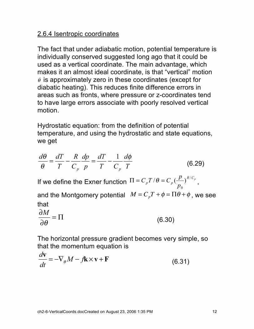
2.6.4 Isentropic coordinates The fact that under adiabatic motion, potential temperature is individually conserved suggested long ago that it could be used as a vertical coordinate. The main advantage, which makes it an almost ideal coordinate, is that “vertical” motion !! is approximately zero in these coordinates (except for diabatic heating). This reduces finite difference errors in areas such as fronts, where pressure or z-coordinates tend to have large errors associate with poorly resolved vertical motion. Hydrostatic equation: from the definition of potential temperature, and using the hydrostatic and state equations, we get

T

d

CT

dT

p

dp

C

R

T

dTd

pp

!

"

" 1#=#= (6.29)

If we define the Exner function pCR

ppp

pCTC

/

0

)(/ ==! " ,

and the Montgomery potential M = CpT + ! = "# + ! , we see that

!="

"

#

M

(6.30)

The horizontal pressure gradient becomes very simple, so that the momentum equation is d

M fdt

!= "# " $ +

vk v F (6.31)


The continuity equation is

ln . 0d p

dt!

!

! !

" "+# + =

" "v

!

(6.32)

The potential vorticity is conserved for adiabatic, frictionless flow (Ertel’s theorem). This general property can be posed in its simplest formulation in isentropic coordinates:

0=dt

dq, (6.33)

where

( . )q fp

!

!"= + # $

"k v , and integrating between two isentropic

surfaces, the potential vorticity is ( . )f

qp

!+ " #

=$

k v

, (6.34)

similar to the shallow water equations potential vorticity. Although the isentropic coordinates have many advantages, they have also two main disadvantages: The first is that isentropic surfaces intersect the ground (as do other vertical coordinates except for sigma-type coordinates). In practice this implies that it is difficult to enforce strict conservation of mass, and this is important for long (climate) integrations. For this reason, hybrid sigma-theta coordinates have been used (e.g., Johnson et al, 1993). Other approaches have been those of Bleck and Benjamin (1993) for the operational RUC/MAPS model, and that of Arakawa and Konor (1996).


The second disadvantage is that only statically stable solutions are allowed, since the vertical coordinate has to vary monotonically with height. There are situations, e.g., over hot surfaces, where this is not true even at a grid-scale. Moreover, in regions of low static stability, the vertical resolution of isentropic coordinates can be low.

Documents

Chapter 2. The continuous equations 2.6 Primitive