14

Chapter 2: Rigid Bar Supported by Two Buckled Struts under Axial,

Harmonic, Displacement Excitation

2.1 Introduction

The model studied in this chapter is a simple system of two buckled struts supporting a

bar that is assumed to be rigid. As mentioned previously, the main difference between

the work in this research and the previous work performed on buckled struts as vibration

isolators by Alloway (2003), Plaut et al. (2003), and Sidbury (2003) is that the system is

comprised of two struts connected by a rigid bar, instead of one strut supporting a mass.

The previous work determined that the behavior of the buckled strut under axial,

harmonic, displacement excitation was similar for fixed-end conditions versus pinned end

conditions of the struts (Sidbury, 2003). Therefore, fixed-end boundary conditions were

chosen for this research because they can support more load and are easier to model

physically.

The first step is to develop and analyze the simple system of a symmetric bar supported

by two buckled struts. The system is analyzed first to obtain the equilibrium state, and

these results are used to analyze the system under forced vertical harmonic excitation at

the base. Because the system is symmetric and there is no rotation of the bar, the

analytical procedure and results are the same as for the fixed-end buckled single-strut

case of the previous work mentioned above. Next, the rigid bar is assumed to be

asymmetric, which loads each strut differently and creates a rotation of the bar. Again,

the system is first evaluated for the equilibrium state, and the results are used to analyze

the response under forced harmonic excitation at the base. Finally, with the bar

remaining asymmetric, the stiffnesses of the vertical struts are varied so there is no

rotation of the bar in equilibrium, and the system is analyzed in the same way as the first

two models.

2.2 General Model Description

All the equations presented in this paper were developed by Dr. Raymond H. Plaut.

Figure 2.1 shows the general model to be analyzed, in an undeformed state.

15

Figure 2.1 Rigid Bar Supported by Fixed-End Struts – Undeformed Shape

The variables used to describe the model are as follows:

L = the length of each strut, assumed to be equal

H = the distance from the bottom of the rigid bar to its centroid when A = 0

A = the distance from the reference line 2H above the bottom of the rigid bar to

the top of the rigid bar at either end.

B1 = the distance from the left end of the rigid bar to its centroid

B2 = the distance from the right end of the rigid bar to its centroid

Φ = the angle of rotation of the rigid bar, measured from the horizontal

When A is equal to zero, the height of the rigid bar is 2H, B1 is equal to B2, and the angle

of rotation Φ is equal to zero. This will be considered a symmetric rigid bar, and is the

first case to be analyzed.

2. 3 Symmetric Bar

2.3.1 Equilibrium Analysis Procedure

The first step of the analysis is to evaluate the model at static equilibrium in a post

buckled state. The model in a post-buckled static equilibrium state is shown in Figure

16

2.2. It should be noted that the model is constrained against any lateral movement. If it

is free to move laterally, the model is unstable and would buckle under sway.

Figure 2.2 Post-Buckled Strut Equilibrium – Symmetric Bar

Because the bar is symmetric and the struts are assumed to have the same length and

bending stiffness, analysis is done on one strut, and the other strut is assumed to be its

mirror image. Figure 2.3 shows a single buckled strut in a horizontal position.

Figure 2.3 Single Buckled Strut Under Static Load Po

The post-buckled state is achieved by loading the strut just above its Euler buckling load.

(Hence, the full model will be loaded at twice this value, because there are two struts.)

The strut is assumed to be an elastica, which means there is no axial deformation of the

strut along its length. When the strut is evaluated in the equilibrium state, it is permitted

17

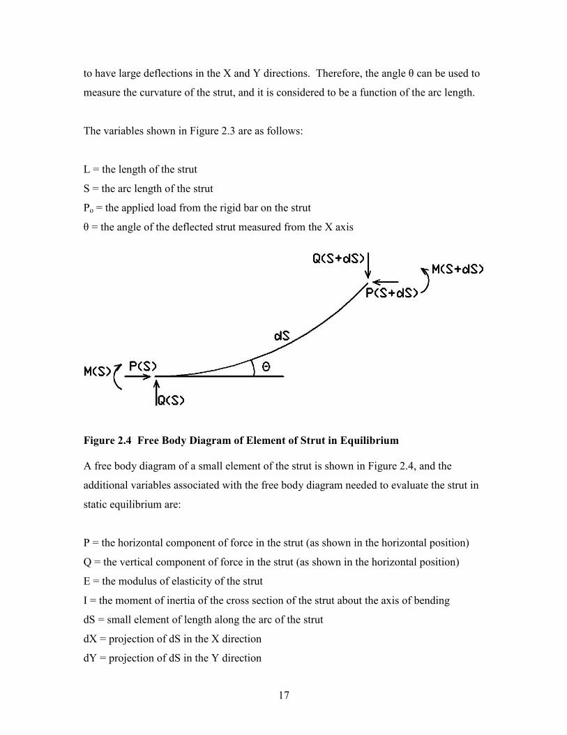
to have large deflections in the X and Y directions. Therefore, the angle θ can be used to

measure the curvature of the strut, and it is considered to be a function of the arc length.

The variables shown in Figure 2.3 are as follows:

L = the length of the strut

S = the arc length of the strut

Po = the applied load from the rigid bar on the strut

θ = the angle of the deflected strut measured from the X axis

Figure 2.4 Free Body Diagram of Element of Strut in Equilibrium

A free body diagram of a small element of the strut is shown in Figure 2.4, and the

additional variables associated with the free body diagram needed to evaluate the strut in

static equilibrium are:

P = the horizontal component of force in the strut (as shown in the horizontal position)

Q = the vertical component of force in the strut (as shown in the horizontal position)

E = the modulus of elasticity of the strut

I = the moment of inertia of the cross section of the strut about the axis of bending

dS = small element of length along the arc of the strut

dX = projection of dS in the X direction

dY = projection of dS in the Y direction

18

Using the variables described above, the following equations can be written to describe

the shape of the strut:

θcos=dS

dX (2.1)

θsin=dS

dY (2.2)

CurvaturedS

d=

θ (2.3)

dS

dEIM

θ= (2.4)

θθ cossin QPdS

dM+−= (2.5)

All of the analysis is performed in nondimensional terms. The variables have been

nondimensionalized so that the analysis provides valid results for any elastic material

regardless of its value of modulus of elasticity E, and for any cross-sectional shape

regardless of its value of moment of inertia I. In this way, results are not limited to

specific materials or cross-sectional shapes. The variables have been nondimensionalized

as follows:

L

Xx =

L

Yy =

L

Ss = (2.6, 2.7, 2.8)

EI

QLq

2

= EI

PLp

2

= EI

MLm = (2.9, 2.10, 2.11)

To obtain a post-buckled state of interest, the strut should be loaded slightly above the

buckling load. For a strut with fixed-end conditions at both ends, this critical load is Po =

42 EI/L

2 . The nondimensional buckling load, pcr = PoL

2 /EI has the value pcr = 4

2 ≈

39.478. A static value of po = 40 will be used in the analysis. (Hence, an initial

nondimensional load of po = 80 will be applied to the entire system because there are two

struts.) When the nondimensional variables shown in Equations 2.6 through 2.11 are

19

used in Equations 2.1, 2.2, 2.4, and 2.5, the result is the following differential equations

for 0 < s < 1:

θcos=ds

dx (2.12)

θsin=ds

dy (2.13)

mds

d=

θ (2.14)

θθ cossin qpds

dm+−= (2.15)

Boundary conditions must be established to complement the differential equations. The

fixed-end condition of the strut does not allow any rotation at the ends of the strut, nor

does it allow any deflection in the y direction (as shown in the horizontal position).

Therefore, the boundary conditions used to solve the system of differential equations for

the fixed-end condition are as follows:

At s = 0: x = 0, y = 0, and θ = 0 (the left, or bottom, end of the strut)

At s = 1: y = 0, and θ = 0 (the right, or top, end of the strut)

A Mathematica program was written to solve the system of equations. Based on a given

value for the initial load po, the program solves for the values of the moment m and the

shear force q at the left end, or bottom, of the strut (at s = 0). The program utilizes a

shooting method, which is an iterative process in which initial guesses are given for m

and q, and the solution is found by an iterative procedure. A text printout of the program

is provided in Appendix A.

2.3.2 Dynamic Analysis Procedure

The model is subjected to a forced harmonic vibration (axial base displacement), as

discussed in Chapter 1, given by Equation 1.1. Again, showing the strut in the horizontal

20

position in Figure 2.5, the base is at the left, and the excitation is shown acting on the

base. The reaction force at the top (or right end) is given as the mass of the system

(weight W divided by the gravitational acceleration g) multiplied by the acceleration of

the system, which is the second derivative of the position function (refer to Equation 1.5)

plus the static force W. Note that now the deflection is a function of position along the

strut and time.

Figure 2.5 Strut Under Forced Harmonic Vibration

The variables used in the dynamic analysis are listed below:

T = time

W = weight of supported load (half of rigid bar)

Ω = applied frequency

Uosin(ΩT) = axial displacement of base of strut (in X direction)

g = acceleration of gravity

µ = mass per unit length of the strut

Pw = the ratio of the weight W to the weight µgl of the strut

r = stiffness parameter

C = external damping coefficient

The new variables introduced above are also nondimensionalized in the same way as the

first set of variables in Equations 2.6 – 2.11. These equations are shown below:

Time: 4L

EITt

µ= (2.16)

21

Frequency: EI

L4µω Ω= (2.17)

Base Displacement Amplitude: L

Uu o

o = (2.18)

Forces: gL

Wpw

µ= ,

EI

WLpo

2

= (2.19, 2.20)

Stiffness Parameter: 3gL

EI

p

pr

o

w

µ== (2.21)

External Damping Parameter: EI

CLc

µ

2

= (2.22)

Damping is assumed to be viscous damping, i.e., the relationship between the damping

force and the velocity of the system is linear. Damping will not be varied much within

the experiments to be performed. This is due to the fact that damping is difficult to

model. It can not be determined from the size, dimensions, material, or other physical

properties of an element. It must be determined through experiments such as a free-

vibration test. But it is present and must be accounted for in the analysis.

To analyze the strut under forced harmonic excitation, a free body diagram of forces

acting on an element at a particular time and position can be drawn. This is done using

D’Alembert’s Principle, which uses a fictitious inertia force that is equal to the product

of the mass and the acceleration. This force is assumed to act in the opposite direction of

the accelerating mass, therefore at a particular instant in time, the strut is considered to be

in a state of static equilibrium (Chopra, 2001). The damping force is also included in the

free body diagram - see Figure 2.6.

22

Figure 2.6 Free Body Diagram of Element of Strut Under Forced Harmonic

Vibrations

Using this free body diagram, the following relationships can be written (prior to

nondimensionalizing the terms):

θcosS

X=

∂

∂ (2.23)

θsin=∂

∂

S

Y (2.24)

EI

M

S=

∂

∂θ (2.25)

θθ cossin QPS

M+−=

∂

∂ (2.26)

T

XC

T

X

S

P

∂

∂−

∂

∂−=

∂

∂2

2

µ (2.27)

T

YC

T

Y

S

Q

∂

∂−

∂

∂−=

∂

∂2

2

µ (2.28)

23

The following differential equations can now be written using the equilibrium

relationships, for values of s between 0 and 1:

θcos=∂

∂

s

x (2.29)

θsin=∂

∂

s

y (2.30)

ms=

∂

∂θ (2.31)

ss

m

∂

∂=

∂

∂ θ (2.32)

t

xc

t

x

s

p

∂

∂−

∂

∂−=

∂

∂2

2

(2.33)

t

yc

t

y

s

q

∂

∂−

∂

∂−=

∂

∂2

2

(2.34)

Each variable that describes the strut can now be written as a function of time and

location along the strut to describe the response of the strut to the forced excitation. The

subscript “e” represents the equilibrium portion of the equation, and “d” represents the

dynamic portion. These equations, in nondimensional terms, are written below:

ti

de esxsxtsx ω)()(),( += (2.35)

ti

de esysytsy ω)()(),( += (2.36)

ti

de essts ωθθθ )()(),( += (2.37)

ti

de esmsmtsm ω)()(),( += (2.38)

ti

do espptsp ω)(),( += (2.39)

ti

de esqqtsq ω)(),( += (2.40)

24

It is assumed that the dynamic vibrations will be very small, and small displacement

theory can be used to determine the following linear dynamic relationships:

edd sin

ds

dxθθ−= (2.41)

edd cos

ds

dyθθ= (2.42)

dd m

ds

d=

θ (2.43)

edededodd sin)qp(cos)pq(

ds

dmθθθθ +−−= (2.44)

dd xci

ds

dp)( 2 ωω −= (2.45)

dd yci

ds

dq)( 2 ωω −= (2.46)

The final equations required to solve the system of differential equations are the

boundary conditions at each end of the strut. In nondimensional terms, they are:

At s=0: xd = uo, yd = 0, θd = 0 (the left, or bottom end of the strut)

At s=1: yd = 0, θd = 0 (the right, or top end of the strut)

A program was written in Mathematica to solve the system of differential equations,

similar to the program used to solve the static equilibrium equations. The values for the

moment me and shear force qe determined from the equilibrium analysis are used as input

in the dynamic analysis to determine the transmissibility. Also, known values of the

initial load po, the amplitude of the excitation at the base uo, the stiffness parameter r, and

the external damping parameter c are used as input in the program. It then utilizes a “do”

loop to solve for the transmissibility of the system for a range of nondimensional

frequency values, ω. As before, it uses a shooting method to solve the equations. Initial

guesses are given for the values of pd(0), qd(0), and md(0). To aid in the speed of the

program, the results for the values of pd(0), qd(0), and md(0), or some percentage of their

25

values, are then used as the guess for the next run in the loop. Appendix B shows a text

printout of this program.

The transmissibility of the system is the ultimate goal of this calculation, and indeed this

research as a whole. The equation used to determine the transmissibility is shown below

o

2

dm

2

d

u

)]1(x[I)]1(xRe[TR

+= (2.47)

As mentioned before, this is a displacement transmissibility. The equation utilizes the

capabilities of the computer program to solve for the real and imaginary parts of the

solution. The resulting value used for the position of the strut at the top due to the

dynamic load is the square root of the sum of the squares (SRSS) of the real and

imaginary values. This, of course, is divided by the original amplitude of the base, uo, to

determine the transmissibility. Because each strut is forced at the same amplitude and

frequency, the transmissibility calculated for the top of each strut is also the

transmissibility at the center of the rigid bar.

Another useful characteristic of the system to determine are its resonant frequencies. A

resonant frequency can be determined by locating a frequency at which an undamped

system’s transmissibility is infinite. By setting the value of the external damping

parameter c equal to zero, the undamped case can be analyzed and the resonant

frequencies can be found. When transmissibility is plotted versus the nondimensional

frequency ω, the resonant frequencies are easily located in the undamped case by the

high peaks on the plot. Also, as long as the system’s damping is below the critical

damping value, the transmissibility plots for damped cases will still show peaks near

these resonant frequency locations. (A system is considered critically damped or

overdamped when it does not oscillate under a free vibration situation.) As the value of c

increases and approaches its critical value, the transmissibility at a resonant frequency

tends to decrease.

26

2.3.3 Results for Symmetric Bar

The transmissibility of the system was calculated for a range of nondimensional applied

frequencies from 0.1 to 200. For the case c = 1, r = 1, and po = 40, it is plotted against the

frequency in Figure 2.7. As can be seen, four peaks in the transmissibility values are

noted. These peak frequencies are located at ω = 0.69, 44.7, 75.3, and 173.7. It was

mentioned previously that a vibration isolator is only useful when the transmissibility is

below unity. As can be seen in the plot, there is a wide range of frequencies for which

this is the case. For values of ω between approximately 1 and 70, the transmissibility is

well below a value of 1. The transmissibilities of the peak frequencies other than the first

peak are equal to or below 1 as well.

It is also interesting to observe the vibration of the model at each of these peak

frequencies. This is also shown in Figure 2.7. The dark line in each of the vibration

shapes shows the model in equilibrium, before it is subjected to the harmonic excitation.

The two lighter lines show the shape of the vibrating struts at each peak frequency. The

vibration shape at the first peak, ω = 0.69, shows greater movement of the rigid bar

above and below the equilibrium state compared to the other three shapes. This is

expected because the transmissibility at this peak is much higher. The vibration shape of

the struts at ω = 0.69 is similar to the equilibrium shape, i.e., there are no nodes. The

vibration shapes of the struts at the second and fourth peak frequencies show very

noticeable nodes. One node is present at the second peak, and three nodes can be seen at

the fourth peak. It is interesting to note that there are no nodes at the third peak.

27

Displacement Transmissibility vs. Frequency

Symmetric Case (c=1, r=1, po=40)

0.001

0.01

0.1

1

10

100

0.1 1 10 100 1000

Frequency, ω

Transmissibility

ω=0.69

ω=44.7

ω=75.3

Vibration at ω=75.3

Vibration at ω=44.7Vibration at ω=0.69

ω=173.7

Vibration at ω=173.7

Figure 2.7 Transmissibility vs. Frequency with Vibration Shapes

28

2.4 Asymmetric Bar

The case of the perfectly symmetric rigid bar is of course ideal, but is useful for studying

the effectiveness of post-buckled struts as vibration isolators. Results from Sidbury

(2003) are applicable for the symmetric case. Because physical objects are rarely

perfectly symmetrical, it was decided to study the performance of the buckled struts

supporting an asymmetric load. Referring to Figure 2.1, a value of A is given other than

zero so that the bar is asymmetrical. Now B1 does not equal B2, and if A is positive, the

centroid of the bar shifts to the right of center. Also, there is now rotation of the bar. A

constant density of the bar is assumed, so that the center of mass is at the same location

as the geometric centroid. Therefore, each strut is supporting a different static load. The

system can no longer be analyzed by evaluating one strut because the struts are no longer

mirror images of each other. As before, the system must be analyzed in an equilibrium

state first, and then the solutions from the equilibrium analysis are used in the dynamic

analysis.

2.4.1 Equilibrium Analysis Procedure

Figure 2.8 below shows the system in its deformed shape under the applied static load.

As before, it is constrained against lateral movement for stability.

Figure 2.8 Post-Buckled Equilibrium State – Asymmetric Case

29

The same nondimensional quantities used in the single-strut analysis will be used here,

except each strut will have its own set of variables, designated by a subscript 1 for the left

strut and 2 for the right strut:

L

Xx 11 = ;

L

Xx 22 =

L

Yy 11 = ;

L

Yy 22 = (2.48, 2.49, 2.50, 2.51)

L

Ss 11 = ;

L

Ss 22 =

EI

LQq

2

11 = ;

EI

LQq

2

22 = (2.52, 2.53, 2.54, 2.55)

EI

LPp

2

11 = ;

EI

LPp

2

22 =

EI

LMm 1

1 = ; EI

LMm 2

2 = (2.56, 2.57, 2.58, 2.59)

In addition, the following variables are nondimensionalized:

L

Aa =

L

Hh =

L

Bb 11 = (2.60, 2.61, 2.62)

L

Bb 22 =

EI

WLpo

2

2

= (2.63, 2.64)

A free body diagram of the rigid bar is drawn in Figure 2.9 to show the forces acting in

static equilibrium. The forces from the struts are at s = 1 (top of the strut). In the

symmetric case, m1 and m2 were equal and opposite values, and p1 equaled p2 which

equaled po. When the bar is asymmetric, this is not the case. Separate values must be

determined for each strut.

Figure 2.9 Free Body Diagram of Static Forces on Rigid Bar

30

From the free body diagram shown above, the following equations are written:

oppp 221 =+ (2.64)

021 =+ qq (2.65)

)]1()1()[(

)]1()1()[2()]1()1()[(

2121

12112221211122

mmbb

xxhpbqbqyybbbpbp o

++

=−+−+−++− (2.66)

21

12 )1()1(sin

bb

xx

+

−=φ (2.67)

1)1()1(

cos21

21 ++

−=

bb

yyφ (2.68)

Also, the same equations written from the free body diagram of the single strut will apply

to the struts (Equations 2.12 – 2.15). But again, each strut will have its own set of

equations, using the same subscript notation:

1

1

1 cosθ=ds

dx 2

2

2 cosθ=ds

dx (2.69, 2.70)

1

1

1 sinθ=ds

dy 2

2

2 sinθ=ds

dy (2.71, 2.72)

1

1

1 mds

d=

θ 2

2

2 mds

d=

θ (2.73, 2.74)

1111

1

1 cossin θθ qpds

dm+−= 2222

2

2 cossin θθ qpds

dm+−= (2.75, 2.76)

31

The final set of equations needed to solve the differential equations are the boundary

conditions at the ends of each strut. Assuming fixed-end conditions, they are as follows:

At s1,2 = 0: x1,2 = 0, y1,2 = 0, θ1,2 = 0

At s1,2 = 1: 21

122,1

)1()1(sin

bb

xx

+

−=θ 1

)1()1(cos

21

212,1 +

+

−=

bb

yyθ

For the boundary condition equation used at the top of the strut (s = 1), it has been

assumed that the angle of rotation Φ of the rigid bar is the same as the angle θ of the

strut. This assumption can be made because the struts are assumed to be fixed to the rigid

bar, which allows no rotation with reference to the strut itself. If the rigid bar rotates, the

struts will rotate by the same amount.

A Mathematica program was again written to solve the system’s differential equations.

As in the case of one strut, the value of the static load po is known. In addition, values are

assigned to “a”, b and h for the rigid bar. The value b = 0.5 is used so that the length of

the bar is equal to the length of each strut. This value is used for all analyses of the

asymmetric bar. By varying the value of “a”, different asymmetric cases can be studied.

A text printout of the Mathematica program can be found in Appendix C.

2.4.2 Equilibrium Results

For verification of the equilibrium program written for the asymmetric case, it was first

evaluated for the symmetric case a = 0. This results in b1=b2, hence the bar is symmetric.

The equilibrium results for the values of the moment and shear force in the struts were

equal for each strut, and their value (m = 2.04 and 0≅q ) was equal to the moment and

shear force values determined for the symmetric case analysis using a single strut.

Therefore, the program was verified for this special case.

It should also be mentioned that the direction of the buckled struts for the symmetric case

can be outward as shown, or inward (the struts would be buckled towards each other

32

rather than away from each other). By giving the program initial guesses of a positive

value for m1 (the left strut) and a negative value for m2 (the right strut), the struts are

buckled away from each other (outward). By reversing the sign of the initial guesses, the

struts are buckled inward. The inward buckled case was analyzed on the model and it did

not change the magnitude of the equilibrium moment or shear force in the struts.

However, when the asymmetric cases were analyzed (a 0≠ ), the program did not give

reasonable values for moments and shears in the struts unless they were buckled outward.

Therefore, the outward buckled case is the appropriate condition for asymmetric

equilibrium and was used for the remainder of the equilibrium and dynamic analysis.

Table 2.1 shows the values of “a” that were used for the dynamic analysis, which will be

discussed later, and the corresponding values of b1. When a = 0, then b1 = 0.5, and the

bar is symmetric.

Table 2.1 Values of “a” and the Corresponding b1 Value

a 0 0.008 0.02 0.04 0.06 0.08

b1 0.5 0.52 0.55 0.60 0.65 0.70

The larger the value of b1, the more asymmetry there is in the bar, hence the more the

right strut is loaded than the left. The equilibrium program was run for several values of

“a” between each of those listed in Table 1 above. The equilibrium program solves for

values of p1, q1, m1, and m2. Values of p2 and q2 can then be obtained by Equations 2.63

and 2.64, respectively. Figures 2.10 – 2.14 show how the values of p1, q1, m1, m2, and

the rotation of the bar Φ change as the value of b1 increases from 0.5 to 0.7. Values of b1

above 0.7 were not calculated because the rotation is significant at this point, and it

would be unrealistic to have a system with a significant amount of rotation in its

equilibrium state.

33

Left Strut Axial Load p1 vs. b1

(po = 40)

20

22

24

26

28

30

32

34

36

38

40

0.5 0.52 0.54 0.56 0.58 0.6 0.62 0.64 0.66 0.68 0.7

b1

Axial Load p1

Figure 2.10 Left Strut Axial Load p1 vs. b1

As expected, the axial load on the left column decreases as the value of b1 increases,

because the center of mass of the rigid bar is moving away from the left strut. If the axial

load of the right strut, p2, were plotted, it would show the mirror image about p1 = 40

because the sum of p1 and p2 is 2po. Because the stiffness of each strut remains the same,

the Euler buckling load for each column is still equal to 40. Therefore, the left strut is

below the buckling load in all of these cases, and the post-buckled stiffness

characteristics required for the system to behave as a vibration isolator are only present in

the right strut. Results of this system’s performance will be discussed later in the chapter.

34

Shear Force of Left Strut q1 vs. b1

(po = 40)

-1.8

-1.6

-1.4

-1.2

-1.0

-0.8

-0.6

-0.4

-0.2

0.0

0.5 0.52 0.54 0.56 0.58 0.6 0.62 0.64 0.66 0.68 0.7

b1

Shear Force q1

Figure 2.11 Shear Force of Left Strut q1 vs. b1

By observing Figure 2.11, we can see that the magnitude of shear force begins to increase

dramatically as the value of b1 increases. Only the left strut shear force is plotted because

the right strut shear force is equal and opposite in value. The negative sign only gives the

force its direction; the shear force magnitude increases in both struts as the bar becomes

more asymmetric. This would be the case for a shift in the center of mass to the left as

well as to the right of the center of the bar.

35

Left Strut Moment m1 vs. b1

(po = 40)

1.70

1.75

1.80

1.85

1.90

1.95

2.00

2.05

2.10

0.5 0.52 0.54 0.56 0.58 0.6 0.62 0.64 0.66 0.68 0.7

b1

m1

Figure 2.12 Left Strut Moment m1 vs. b1

Right Strut Moment m2 vs. b1

(po = 40)

-9

-8

-7

-6

-5

-4

-3

-2

-1

0

0.5 0.52 0.54 0.56 0.58 0.6 0.62 0.64 0.66 0.68 0.7

b1

m2

Figure 2.13 Right Strut Moment m2 vs. b1

36

For the symmetric case, the moment in each strut is equal and opposite, and the

magnitude is approximately 2.04 when a value of initial load of 40 is used. For the

asymmetric case, the moments are not equal and opposite, nor do they vary with the

value of b1 in a similar way. Looking at Figure 2.12, the left strut moment decreases

sharply for a slight offset of symmetry, and then increases slightly and levels out at a

value of approximately 1.85 until the center of mass has shifted a significant distance to

the right of center. However, the right strut moment, shown in Figure 2.13 with a

different scale on the ordinate, continues to steadily increase in magnitude (note that the

values for the moment are negative) as the center of mass moves closer to the right strut.

This is an interesting observation, considering that the axial load in each strut steadily

increases or decreases.

The final plot developed is Figure 2.14, which shows how the angle of rotation (in

radians) of the bar changes with the shift in center of mass. As expected, the rotation

steadily increases. This can also be seen in the deflected shape of the system at

equilibrium for different values of b1 in Figure 2.15.

Rotation of Rigid Bar vs. b1

(po = 40)

0

0.05

0.1

0.15

0.2

0.25

0.3

0.35

0.5 0.52 0.54 0.56 0.58 0.6 0.62 0.64 0.66 0.68 0.7

b1

Rotation

Figure 2.14 Rotation of Rigid Bar vs. b1

37

Deformed Shape at

Equilibrium - b1=0.55Deformed Shape at

Equilibrium - b1=0.60

Deformed Shape at

Equilibrium - b1=0.65

Deformed Shape at

Equilibrium - b1=0.70

Figure 2.15 Deformed Shape of Model for Different Values of b1

2.4.3 Dynamic Analysis Procedure

2.4.3.1 Strut Equations

The same equations (Equations 2.35 – 2.40) used to describe the response of the single

strut due to a forced harmonic excitation (written as a function of time and location along

the strut) are applicable in the asymmetric case as well, except that each strut must have

its own set of independent equations. These equations, in nondimensional terms, are

written as follows:

38

ti

de esxsxtsx ω)()(),( 111111 += ti

de esxsxtsx ω)()(),( 222222 += (2.77,2.78)

ti

de esysytsy ω)()(),( 111111 += ti

de esysytsy ω)()(),( 222222 += (2.79, 2.80)

ti

de essts ωθθθ )()(),( 111111 += ti

de essts ωθθθ )()(),( 222222 += (2.81, 2.82)

ti

de esmsmtsm ω)()(),( 111111 += ti

de esmsmtsm ω)()(),( 222222 += (2.83, 2.84)

ti

do espptsp ω)(),( 11111 += ti

do espptsp ω)(),( 22222 += (2.85, 2.86)

ti

de esqqtsq ω)(),( 11111 += ti

de esqqtsq ω)(),( 22222 += (2.87, 2.88)

Therefore, Equations 2.41-2.46 can also be used, one set for each strut:

ed

d

ds

dx11

1

1 sinθθ−= ed

d

ds

dx22

2

2 sinθθ−= (2.89, 2.90)

ed

d

ds

dy11

1

1 cosθθ= ed

d

ds

dy22

2

2 cosθθ= (2.91, 2.92)

d

d mds

d1

1

1 =θ

d

d mds

d2

2

2 =θ

(2.93, 2.94)

edededod

d qppqds

dm11111111

1

1 sin)(cos)( θθθθ +−−= (2.95,2.96)

edededod

d qppqds

dm22222222

2

2 sin)(cos)( θθθθ +−−= (2.97,2.98)

d

d xcids

dp1

2

1

1 )( ωω −= d

d xcids

dp2

2

2

2 )( ωω −= (2.99,2.100)

d

d ycids

dq1

2

1

1 )( ωω −= d

d ycids

dq2

2

2

2 )( ωω −= (2.101,2.102)

2.4.3.2 Rigid Body Equations

Applying D’Alembert’s Principle again, a free body diagram of the inertial forces on the

rigid bar is drawn in Figure 2.16, along with the static forces. Note that now the variables

39

associated with the bar are all functions of time, and the variables along each strut are

functions of position on the strut and time.

Figure 2.16 Free Body Diagram of Rigid Bar Under Forced Harmonic Vibrations

The following relationships are developed from the free body diagram shown in Figure

2.16

WTLPTLPdT

TXdM −+= ),(),(

)(212

2

(2.103)

),(),()(

212

2

TLQTLQdT

TYdM += (2.104)

)](sin)(cos)[,()](sin)(cos)[,()(

11222

2

THTBTLPTHTBTLPdT

TdI o φφφφ

φ−−+=

),(),(

)](cos)(sin)[,()](cos)(sin)[,(

21

1122

TLMTLM

THTBTLQTHTBTLQ

−−

+−−+ φφφφ (2.105)

)(sin)(cos),()( 11 TBTHTLXTXHL φφ ++=++ (2.106)

)(sin)(cos),( 22 TBTHTLX φφ −+=

)(cos)(sin),()( 222 TBTHTLYTYB φφ ++=+

)(cos)(sin),( 1121 TBTHTLYBB φφ −+++= (2.107)

40

From Equations 2.106 and 2.107,

21

12 )],(),([)(sin

BB

TLXTLXT

+

−=φ (2.108)

21

2121 )],(),([)(cos

BB

TLYTLYBBT

+

−++=φ (2.109)

By substituting Equations 2.108 and 2.109 into Equation 2.105 and evaluating at X=L,

we obtain

=2

2 )(

dT

TdI o

φ

)(

)],(),(][),(),(),(),([

21

2121121122

BB

TLYTLYBBHTLQHTLQBTLPBTLP

+

−++−−−

)(

)],(),(][),(),(),(),([

21

12121122

BB

TLXTLXHTLPHTLPBTLQBTLQ

+

−++−+

),(),( 21 TLMTLM −− (2.110)

The final nondimensional quantity to be defined is for the moment of inertia of the bar, Io,

which is defined as

221

242222124

23)

2(

12482)

2([

3

2 bbaaahbbhh

h

rp

L

Ii ooo

+−−+

++==

µ (2.111)

This nondimensional quantity, along with the other nondimensional quantities presented

in Equations 2.16-2.22 and 2.48 – 2.64, can be used to rewrite Equations 2.103, 2.104,

and 2.106 – 2.109 in nondimensional terms:

0

021

2

2

2

]2),1(),1([)(

rp

ptptp

dt

txd −+= (2.112)

orp

tqtq

dt

tyd

2

)],1(),1([)( 21

2

2 += (2.113)

)(sin)(cos),1()(1 11 tbthtxtxh φφ ++=++ (2.114)

)(sin)(cos),1( 22 tbthtx φφ −+=

41

)(cos)(sin),1()( 222 tbthtytyb φφ ++=+ (2.115)

)(cos)(sin),1( 1121 tbthtybb φφ −+++=

21

12 )],1(),1([)(sin

bb

txtxt

+

−=φ (2.116)

21

2121 )],1(),1([)(cos

bb

tytybbt

+

−++=φ (2.117)

)(

)],1(),1(][),1(),1(),1(),1([)(

21

2121121122

2

2

bb

tytybbhtqhtqbtpbtp

dt

tdio

+

−++−−−=

φ

)(

)],1(),1(][),1(),1(),1(),1([

21

12121122

bb

txtxhtphtpbtqbtq

+

−++−+

),1(),1( 21 tmtm −− (2.118)

2.4.3.3 Boundary Conditions

To develop expressions for the boundary conditions at s1 = s2 = 1; the strut and rigid body

equations listed above are manipulated as follows:

If Equations 2.116 and 2.117 are substituted into Equation 2.114, the following

expression results (for s1 = 1):

1)],1(),1(),1(),1([

)(21

212112 −+

−++=

bb

thythytxbtxbtx (2.119)

The second derivative is then

]),1(),1(),1(),1(

[)(

1)(2

2

2

2

1

2

2

2

2

12

1

2

2

21

2

2

t

tyh

t

tyh

t

txb

t

txb

bbdt

txd

∂

∂−

∂

∂+

∂

∂+

∂

∂

+= (2.120)

When Equation 2.120 above is set equal to Equation 2.112, (because both are expressions

for the second derivative of x(t)), the second derivatives with respect to time t of

42

Equations 2.77 – 2.80 and 2.85, 2.86 are substituted appropriately (hence eliminating the

equilibrium portion), and the [eiωt]2 term is cancelled from both sides (since we are

conducting a linear dynamic analysis), the following expression results:

)]1()1()[()1()1()1()1([2 2121212112

2

ddddddo ppbbhyhyxbxbrp ++=−++− ω (2.121)

The same manipulation is done for the y component and the Φ component, resulting in

the following equations:

)]1()1()[()1()1()1()1([2 2121122112

2

ddddddo qqbbhxhxybybrp ++=−++− ω (2.122)

hqhqbpbpyybb

xxidddd

ee

ddo )1()1()1()1()]1()1([

)]1()1([121122

2121

21

2

−−−=−++

−ω

)(

])1()1()1()1()][1()1([

21

12112221

bb

hqhqbpbpyy ddddee

+

−−−−+

)(

])1()1()1()1()][1()1([

21

12112221

bb

hqhqbpbpyy eeeedd

+

−−−−+

)(

)]1()1(][)1()1()1()1([

21

121122211

bb

xxbqbqhphp eedddd

+

−−+++

)1()1()(

)]1()1(][)1()1(2[21

21

121122

dd

ddeeo mmbb

xxbqbqhp−−

+

−−++ (2.123)

Using trigonometric identities to manipulate Equations 2.116 and 2.117, and substituting

the equilibrium relations for sinΦe and cosΦe , evaluating at s1 = s2 = 1 gives the

boundary condition

eddedd yyxx φφ cos)]1()1([sin)]1()1([ 1212 −=− (2.124)

As mentioned previously, because the struts are rigidly attached to the bar, and the bar is

also assumed to be rigid, it can be assumed that the angle of rotation of the bar, Φ, is

43

equal to the angles of rotation at the tops of the struts, θ1 and θ2. Therefore, the final two

boundary conditions needed to solve the system of differential equations are

21

12

1

)]1()1([)1(

bb

xx dd

d+

−=θ )1()1( 21 dd θθ = (2.125, 2.126)

Again, a Mathematica program is used to solve the set of differential equations for the

range of nondimensional frequencies 0.1<ω<200. A text printout of the program is given

in Appendix D. Values are set for po, a, h, b, c, and r. The values of p1e, p2e, q1e, q2e, m1e,

and m2e for the given po from the equilibrium analysis are also input values for the

program. Initial guesses are given for the values of p1d, p2d, q1d, q2d, m1d, and m2d at

s1 = 0 or s2 = 0, and the program solves for these values and for the transmissibility for a

given ω. The transmissibility for the system is calculated as an average of the

transmissibilities at the top of each strut, which is the transmissibility at the center of the

rigid bar. This average transmissibility is the value used in all of the transmissibility

versus nondimensional frequency plots presented in the results. The equation for the

transmissibility of each strut is the same as for the single strut (Equation 2.47):

o

dmd

u

xIxTR

2

1

2

1

1

)]1([)]1(Re[ += (2.127)

o

dmd

u

xIxTR

2

2

2

2

2

)]1([)]1(Re[ += (2.128)

2

21 TRTRTRavg

+= (2.129)