CHAPTER 2

Review of Algebra

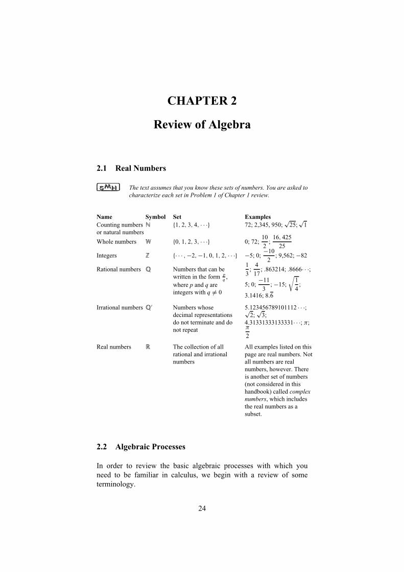
2.1 Real Numbers

The text assumes that you know these sets of numbers. You are asked tocharacterize each set in Problem 1 of Chapter 1 review.

Name Symbol Set ExamplesCounting numbersor natural numbers

� f1, 2, 3, 4, Ð Ð Ðg 72; 2,345, 950;p

25;p

1

Whole numbers � f0, 1, 2, 3, Ð Ð Ðg 0; 72;10

2;

16, 425

25

Integers � fÐ Ð Ð ,�2,�1, 0, 1, 2, Ð Ð Ðg �5; 0;�10

2; 9,562; �82

Rational numbers � Numbers that can bewritten in the form p

q ,where p and q areintegers with q 6D 0

1

3;

4

17; .863214; .8666Ð Ð Ð;

5; 0;�11

3; �15;

√1

4;

3.1416; 8.6

Irrational numbers �0 Numbers whosedecimal representationsdo not terminate and donot repeat

5.123456789101112 Ð Ð Ð;p2;p

3;4.31331333133331Ð Ð Ð; �;�

2

Real numbers � The collection of allrational and irrationalnumbers

All examples listed on thispage are real numbers. Notall numbers are realnumbers, however. Thereis another set of numbers(not considered in thishandbook) called complexnumbers, which includesthe real numbers as asubset.

2.2 Algebraic Processes

In order to review the basic algebraic processes with which youneed to be familiar in calculus, we begin with a review of someterminology.

24

Chapter 2 25

TERM DEFINITION EXAMPLES

Numericalexpression

A number or severalnumbers connectedby definedmathematicaloperations.

6; 5C 2; 5� �p2

Algebraicexpression

A numerical expressionwith at least onevariable.

6x; x C y; 2x2 � 3x C 4

Term A number, a variable,or a product ofnumbers andvariables.

6; x; 6x; 2x2;1

2y3

Polynomial A term or a sum ofterms. (Note: Sincex � y D x C ��y,differences areincluded.)

6; x C y; 4x3 � 3x C 1

Rationalexpression

A polynomial dividedby a nonzeropolynomial. (Note:Includespolynomials, becauseif P is a polynomial,it can be written as

P D P

1.)

x C yx � y ;

1

xC 1

y

Radicalexpression

An algebraicexpression with avariable expressionas a radicand (theexpression under aradical sign).

px; 3py;

√x2 C y2

2

Many of the processes in algebra are based on an agreement, calledthe order-of-operations agreement, that tells us how to deal withexpressions with more than one operation:

First, carry out those operations enclosed in parentheses.Second, carry out all multiplications and divisions as they occur,left to right.

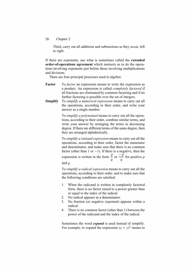
26 Chapter 2

Third, carry out all additions and subtractions as they occur, leftto right.

If there are exponents, use what is sometimes called the extendedorder-of-operations agreement which instructs us to do the opera-tions involving exponents just before those involving multiplicationsand divisions.

There are four principal processes used in algebra:

Factor To factor an expression means to write the expression asa product. An expression is called completely factored ifall fractions are eliminated by common factoring and if nofurther factoring is possible over the set of integers.

Simplify To simplify a numerical expression means to carry out allthe operations, according to their order, and write youranswer as a single number.

To simplify a polynomial means to carry out all the opera-tions, according to their order, combine similar terms, andwrite your answer by arranging the terms in decreasingdegree. If there are different terms of the same degree, thenthey are arranged alphabetically.

To simplify a rational expression means to carry out all theoperations, according to their order, factor the numeratorand denominator, and make sure that there is no commonfactor (other than 1 or �1). If there is a negative, then the

expression is written in the formp

qor�pq

for positive p

and q.

To simplify a radical expression means to carry out all theoperations, according to their order, and to make sure thatthe following conditions are satisfied:

1. When the radicand is written in completely factoredform, there is no factor raised to a power greater thanor equal to the index of the radical.

2. No radical appears in a denominator.3. No fraction (or negative exponent) appears within a

radical.4. There is no common factor (other than 1) between the

power of the radicand and the index of the radical.

Sometimes the word expand is used instead of simplify.For example, to expand the expression �x C y2 means to

Chapter 2 27

simplify it; that is, write

�x C y2 D x2 C 2xy C y2

Evaluate To evaluate an algebraic expression means to replace thevariable or variables with a given number and then simplifythe expression. In calculus, we often evaluate a function attwo values and then we subtract those values. For example,if the function f�x D x2 C x C 1 is evaluated at x D 2,we have f�2 D 22 C 2C 1 D 7, and if f is evaluated atx D 1, we have f�1 D 12 C 1C 1 D 3. Finally, if wesubtract these evaluations, we getf�2� f�1 D 7� 3 D4. Since this is a frequent calculation, a compact notationis sometimes used:

f�xj21 D f�2� f�1

For example,

[x2 C x C 1]j21 D [22 C 2C 1]� [12 C 1C 1]

D 7� 3

D 4

2.3 Powers and roots

EXPONENTS

Definition of Exponent:

In the expression xn, the number n is called the exponent, thenumber b is called the base, and xn is called a power. If n is a

positive integer, then xn D x Ð x Ð x Ð Ð Ð x︸ ︷︷ ︸n factors

, and x0 D 1; x�n D 1

xn

If m and n are integers, then

x1n D npx whenever n

px is defined

and

xmn D �x

1n m D � n

pxm whenever n

px is defined

Factorial numbers:n! D n�n� 1�n� 2 Ð Ð Ð 3 Ð 2 Ð 1 0! D 1 for n a nonnegativeinteger

28 Chapter 2

ROOTS

Recall that for any positive even integer n (called the index of theradical) and any positive number x (called the radicand),

y D npx if and only if y > 0 and yn D x

We call y the positive nth root of x. For example, the positive fourthroot of 16 is denoted by 4

p16; we write 4

p16 D 2, since 24 D 16.

For any positive odd integer n and any number x (positive ornegative),

y D npx and only if yn D x

and y is called the nth root of x. For example, 3p�8 D �2, since

��23 D �8.Note that

px2 D jxj for any number x.

LAWS OF EXPONENTS

If r and s are real numbers, then

xr Ð xs D xrCs

�xrs D xrs whenever xr is meaningful

�xyr D xryr whenever xr and yr are meaningful(x

y

)rD xr

yrwhenever xr and yr are meaningful and yr 6D 0

xr

xsD xr�s whenever xr and xs are meaningful and xs 6D 0

FACTORS AND EXPANSIONS

Difference of squares: a2 � b2 D �a� b�aC bPerfect square: �aC b2 D a2 C 2abC b2

Difference of cubes: a3 � b3 D �a� b�a2 C abC b2Sum of cubes: a3 C b3 D �aC b�a2 � abC b2Perfect cube: �aC b3 D a3 C 3a2bC 3ab2 C b3

Binomial theorem: �aC bn D(n0

)anb0 C

(n1

)an�1bC(

n2

)an�2b2 C Ð Ð Ð C

(nn

)a0bn

Chapter 2 29

where (n0

)D 1,

(n1

)D n

1,

(n2

)D n�n� 1

1 Ð 2 , Ð Ð Ð ,(nr

)D n!

r!�n� r! , Ð Ð Ð ,(nn

)D 1

The following factoring procedure will work for most of thefactoring problems you encounter in calculus:

To factor an expression: First, look for the greatest commonfactor.Next, check to see if the expression is aspecial type:

Difference of squares: x2 � y2 D �x � y�x C yDifference of cubes: x3 � y3 D �x � y�x2 C xy C y2Sum of cubes: x3 C y3 D �x C y�x2 � xy C y2Perfect square: x2 C 2xy C y2 D �x C y2

x2 � 2xy C y2 D �x � y2

Finally, if the expression is a trinomial, factor it into two binomials.Sometimes, grouping the terms will help you to factor.

EXAMPLE 2.1 Common factoring

Factor the following expressions:

a. Common monomial factors: a2bC 5a3b2 C 7a2b3

b. Common binomial factors: 5x�3a� 5bC 9y�3a� 5b

c. Common factoring to provide integral coefficients:1

36x � y

d. Multiple common factoring:

�2x � 3�3�1� x�1C x��1� �1C x3��3

Solution

a. The common factor is a2b:

a2bC 5a3b2 C 7a2b3 D a2b�1C 5abC 7b2

b. The common factor is �3a� 5b:

5x�3a� 5bC 9y�3a� 5b D �5x C 9y�3a� 5b

30 Chapter 2

c. Treat the fraction as a common factor:

1

36x � y D 1

36x � 36

36y

D 1

36�x � 36y

d. The common factor is 3�1C x:

�2x � 3�3�1� x�1C x��1� �1C x3��3

D 3�1C x[�2x � 3�1� x��1� �1C x2��1]

D 3�1C x[�2x � 2x2 � 3C 3x��1C 1C 2x C x2]

D 3�1C x[3x2 � 3x � 2] �

EXAMPLE 2.2 Factoring special types

Factor the following expressions:

a. 3x2 � 75b. �x C 3y3 C 8

c.9a2

b2� �aC 3b2

d. x6 � 1

Solution

a. 3x2 � 75 D 3�x2 � 25 Common factor first

D 3�x � 5�x C 5 Difference of squares

b. Recognize this as a sum of cubes:

�x C 3y3 C 8 D [�x C 3yC 2][�x C 3y2 � �x C 3y�2C �22]

D �x C 3y C 2�x2 C 6xy C 9y2 � 2x � 6y C 4

c. Use common factoring to provide integral coefficients:

9a2

b2� �aC 3b2 D 1

b2[9a2 � b2�aC 3b2] Common factor

D 1

b2[3a� b�aC 3b][3a C b�aC 3b]

Difference of squares

Chapter 2 31

D 1

b2�3a� ab� 3b2�3aC abC 3b2

d. Treat this as a difference of squares.

x6 � 1 D �x32 � �132

D �x3 � 1�x3 C 1

D �x � 1�x2 C x C 1�x C 1�x2 � x C 1 �

EXAMPLE 2.3 Factoring trinomials

Factor the following expressions:a. x2 � 8x C 15 b. 6w2 � 9w� 15c. 6�x C y2 � 9�x C y� 15 d. 4x4 � 13x2y2 C 9y4

Solution

a. x2 � 8x C 15 D �x � 5�x � 3

b. 6w2 � 9w� 15 D 3�2w2 � 3w � 5 Common factor first

D 3�2w� 5�wC 1

c. 6�x C y2 � 9�x C y� 15 D 3[2�x C y2 � 3�x C y� 5]

D 3[2�x C y� 5][�x C yC 1]

D 3�2x C 2y � 5�x C y C 1

d. 4x4 � 13x2y2 C 9y4 D �x2 � y2�4x2 � 9y2

D �x � y�x C y�2x � 3y�2x C 3y �

EXAMPLE 2.4 Factoring using negative exponents

x�12 y

12 � x 1

2 y�12 D x�

12y�

12 �y � x D y � xp

xy�

RADICALS

An algebraic expression containing radicals is simplified if all four ofthe following conditions are satisfied:

32 Chapter 2

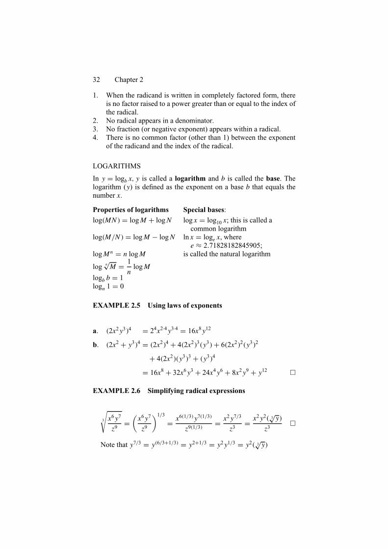
1. When the radicand is written in completely factored form, thereis no factor raised to a power greater than or equal to the index ofthe radical.

2. No radical appears in a denominator.3. No fraction (or negative exponent) appears within a radical.4. There is no common factor (other than 1) between the exponent

of the radicand and the index of the radical.

LOGARITHMS

In y D logb x, y is called a logarithm and b is called the base. Thelogarithm (y) is defined as the exponent on a base b that equals thenumber x.

Properties of logarithms Special bases:

log�MN D logMC logN log x D log10 x; this is called acommon logarithm

log�M/N D logM� logN ln x D loge x, wheree ³ 2.71828182845905;

logMn D n logM is called the natural logarithm

log npM D 1

nlogM

logb b D 1logn 1 D 0

EXAMPLE 2.5 Using laws of exponents

a. �2x2y34 D 24x2Ð4y3Ð4 D 16x8y12

b. �2x2 C y34 D �2x24 C 4�2x23�y3C 6�2x22�y32

C 4�2x2�y33 C �y34

D 16x8 C 32x6y3 C 24x4y6 C 8x2y9 C y12 �

EXAMPLE 2.6 Simplifying radical expressions

3

√x6y7

z9D(x6y7

z9

)1/3

D x6�1/3y7�1/3

z9�1/3D x2y7/3

z3D x2y2� 3

py

z3�

Note that y7/3 D y�6/3C1/3 D y2C1/3 D y2y1/3 D y2� 3py

Chapter 2 33

EXAMPLE 2.7 Simplifying expressions with negative exponents

a. �x�1 C y�1�1 D(

1

xC 1

y

)�1

D(x C yxy

)�1

D xy

x C yb. �x�1y�1�1 D xy �

EXAMPLE 2.8 Expanding an expression by using the binomialtheorem

Expand �2x � 3y5.

Solution In the binomial theorem, replace a by 2x and b by ��3y.With n D 5, we have

�2x � 3y5 D �1�2x5��3y0 C 5�2x4��3y1 C 5 Р42�2x3��3y2

C 5 Р4 Р32 Р3 �2x2��3y3 C 5 Р4 Р3 Р2

2 Р3 Р4 �2x1��3y4

C �1�2x0��3y5

D 32x5 � 240x4y C 720x3y2 � 1080x2y3

C 810xy4 � 243y5 �

2.4 Sequences and Series

This material is required in Chapter 8 of the text. A sequence is a list,as in fs0, s1, s2, Ð Ð Ð , sng; a series is a sum: s0 C s1 C s2 C Ð Ð Ð C an.

Arithmetic sequence If an denotes the nth term, d the commondifference, and n the number of terms, then

an D a1 C �n� 1d

Arithmetic series If An denotes the nth partial sum of anarithmetic sequence, then

An D n

2�a1 C an or An D n

2[2a1 C �n� 1d]

Geometric sequence If gn denotes the nth term, r the commonratio, and n the number of terms, then

gn D g1rn�1 for n ½ 1

34 Chapter 2

Geometric series If Gn denotes the nth partial sum of ageometric sequence, then

Gn D g1�1� rn1� r , r 6D 1

Infinite geometric series If G is the sum of an infinite geometricseries, then

G D g1

1� r0 for jrj < 1

SUMS OF POWERS OF THE FIRST n INTEGERS

You can use these formulas to help find Riemann sums in Chapter 5 ofthe text.

n∑kD1

1 D n

n∑kD1

k D 1C 2C 3C Ð Ð Ð C n D n�nC 1

2

n∑kD1

k2 D 12 C 22 C 32 C Ð Ð Ð C n2 D n�nC 1�2nC 1

6

n∑kD1

k3 D 13 C 23 C 33 C Ð Ð Ð C n3 D n2�nC 12

4

n∑kD1

k4D14C24C34 C Ð Ð Ð C n4 D n�nC 1�2nC 1�3n2 C 3n� 1

30

2.5 SOLVING EQUATIONS

Even though there are many aspects of algebra that are important tothe scientist and mathematician, the ability to solve simple equationsis important to the layperson and can be used in a variety of everydayapplications.

Pay attention to the difference between an expression and an equation.Also, note that ‘‘to solve’’ is not the same as ‘‘to simplify.’’ Anequation is a statement of equality. There are three types of equations:true, false, and open. An open equation is an equation with a variable.

Chapter 2 35

A true equation is an equation that lacks variables and that is true,such as

2C 3 D 5

A false equation is an equation that lacks variables and that is false,such as

2C 3 D 15

Our focus is on open equations — those equations with a variable. Thevalues that make an open equation true are said to satisfy the equationand are called the solutions or roots of the equation. To solve an openequation is to find all replacements for the variable(s) that make theequation true. There are three types of open equations. Those that arealways true, such as

x C 3 D 3C xare called identities. Those that are always false, such as

x C 3 D 4C xare called contradictions. Most open equations, such as

2C x D 15

are true for some replacements of the variable and false for otherreplacements. These are called conditional equations. Generally, whenwe speak of equations, we mean conditional equations. Our concern insolving equations is to find the numbers that satisfy a given equation,so we look for things to do to equations to make the solutions orroots more obvious. Two equations with the same solutions are calledequivalent equations. An equivalent equation may be easier to solvethan the original equation, so we try to get successively simplerequivalent equations until the solution is obvious. There are certainprocedures you can use to create equivalent equations. In this section,we will discuss solving the two most common types of equations youwill encounter: linear and quadratic.

Linear equations : ax C b D 0 �a 6D 0

Quadratic equations : ax2 C bx C c D 0 �a 6D 0

Linear Equations

To solve the first-degree (or linear) equation, isolate the variable onone side. That is, the solution of ax C b D 0 is

x D �ba, where a 6D 0

36 Chapter 2

To solve a linear equation, use the following steps:

Step 1: Use the distributive property to clear the equation of paren-theses. If the equation is a rational expression, multiply both sides bythe appropriate expression to eliminate the denominator. Be sure tocheck the solutions obtained by ‘‘plugging’’ the values back into theoriginal equation.

Step 2: Add the same number to both sides of the equality to obtainan equation in which all of the terms involving the variable are on oneside and all of the other terms are on the other side.

Step 3: Multiply (or divide) both sides of the equation by the samenonzero number to isolate the variable on one side.

EXAMPLE 2.9 Solving a linear equation

Solve 4�x � 3C 5x D 5�8C x.

Solution

4�x � 3C 5x D 5�8C x4x � 12C 5x D 40C 5x

9x � 12 D 40C 5x

4x � 12 D 40

4x D 52

x D 13

Check: 4�13� 3C 5�13 D 145, and 5�8C 13 D 145. �

EXAMPLE 2.10 Solving a rational equation

Solvex C 1

x � 2D x C 2

x � 2.

Solution

�x C 1�x � 2 D �x C 2�x � 2

x2 � 2x C x � 2 D x2 � 4

� x � 2 D �4

Chapter 2 37

� x D �2

x D 2

Notice that x D 2 causes division by 0, so the solution set is empty. �

EXAMPLE 2.11 Solving a literal equation

Solve 4x C 5xy C 3y2 D 10 for x.

Solution

4x C 5xy D 10� 3y2

�4C 5yx D 10� 3y2

x D 10� 3y2

4C 5y, y 6D �4

5�

Quadratic Equations: To solve a second-degree (or quadratic)equation, first obtain a zero on one side. Next, try to factor thequadratic. If it is factorable, set each factor equal to zero and solve. Ifit is not factorable, use the quadratic formula:

HANDBOOK THEOREM 1 Quadratic FormulaThe solution of ax2 C bx C c D 0 is

x D �bšpb2 � 4ac

2a, where a 6D 0 �

Examples 2.12–2.16 here are similar to Problems 7–18 in Problem Set1.1.

EXAMPLE 2.12 Solving a quadratic equation by factoring

Solve 2x2 � x � 3 D 0.

Solution Factoring yeilds �2x � 3�x C 1 D 0. If 2x � 3 D 0, thenx D 3

2 ; if x C 1 D 0, then x D �1. The solution is x D 32 ,�1. �

EXAMPLE 2.13 Solving a quadratic equation by using thequadratic formula

Solve 5x2 � 3x � 4 D 0.

38 Chapter 2

Solution a D 5, b D �3, and c D �4; thus (since the equation doesnot factor),

x D 3šp9� 4�5��4

2�5D 3šp89

10�

EXAMPLE 2.14 Solving a literal equation by using the quadraticformula

Solve x2 C 2xy C 3y2 � 4 D 0 for x.

Solution a D 1, b D 2y, c D 3y2 � 4; thus,

x D �2y š√4y2 � 4�1�3y2 � 4

2�1

D �2y š√16� 8y2

2

D �y š√

4� 2y2 �

EXAMPLE 2.15 Solving an absolute-value equation

Solve j5x C 2j D 12.

Solution Use Property 7 of Table 1.1 in the text to write theabsolute-value equation as two equations:

5x C 2 D 12 5x C 2 D �125x D 10 5x D �14

x D 2 x D �14

5

The solution is x D 2,�14

5. �

Exponential Equations: See Examples 4, 7, and 9 of Section 2.4of the text.

Logarithmic Equations: See Examples 5 and 8 of Section 2.4 ofthe text.

Higher Degree Equations: See Examples 2.36, 2.37, and 2.38 onpp. 40–41.

Trigonometric Equations: See Section 4.7, pp. 71–74.

Chapter 2 39

EXAMPLE 2.16 Solving absolute-value equations

a. Solve j5x C 2j D 12. b. Solve j5� 3wj D �3.

Solutiona. Use property 7 of Table 1.1 in the text to write two equations:

5x C 2 D 12 5x C 2 D �125x D 10 5x D �14

x D 2 x D �14

5

The solution is x D 2,�14

5.

b. Use property 1 of Table 1.1 of the text, jaj ½ a, to see that thereare no real values for w that make this equation true. �

2.6 Completing the Square

In Section 1.1 of the text, this procedure of completing the square isused to find the equation of a circle.

In algebra, the method of completing the square was first introducedas a technique for solving quadratic equations. The method leads to aproof of the quadratic formula. However, when we are working withconic sections, we need to complete the square whenever the conic isnot centered at the origin. (See Chapters 6 and 7 of this Handbook.)Consider

Ax2 C Bx CC D 0

We wish to put this into the form

�xC?2 D some number

To do this, we perform the following steps below:

Step 1: Subtract C (the constant term) from both sides:

Ax2 C Bx D �C

Step 2: Divide both sides by A. (A 6D 0; if A D 0, the equation wouldnot be quadratic.) That is, we want the coefficient of the squared termto be 1. The result of dividing by A is

x2 C B

Ax D �C

A

40 Chapter 2

Step 3: Add

(B

2A

)2

to both sides. That is, take one-half of the

coefficient of the first-degree term, square it, and add it to both sides:

x2 C B

Ax C

(B

2A

)2

D B2

4A2� C

A

Step 4: The expression on the left is now a perfect square and canbe factored: (

x C B

2A

)2

D B2

4A2� C

A

EXAMPLE 2.17 Completing the square

Complete the square for x2 C 2x � 5 D 0.

Solution

x2 C 2x � 5 D 0

x2 C 2x D 5

x2 C 2x C 1 D 5C 1

�x C 12 D 6 �

EXAMPLE 2.18 Completing the square when the expressioninvolves fractions

Complete the square for 3x2 C 5x � 4 D 0.

Solution

3x2 C 5x � 4 D 0

3x2 C 5x D 4

x2 C 5

3x D 4

3

x2 C 5

3x C

(5

6

)2

D 4

3C 25

36(x C 5

6

)2

D 73

36�

Chapter 2 41

EXAMPLE 2.19 Completing the square in two variables

Complete the square in both the x and the y terms:

x2 C y2 C 4x � 9y � 13 D 0

Solution Associate the x and y terms:

�x2 C 4xC �y2 � 9y D 13

�x2 C 4x C 4C(y2 � 9y C 81

4

)D 13C 4C 81

4

�x C 22 C(y � 9

2

)2

D 149

4�

EXAMPLE 2.20 Completing the square in two variables

Complete the square in both the x and the y terms:

2x2 � 3y2 � 12x C 6y C 7 D 0

Solution Associate the x and y terms:

�2x2 � 12xC ��3y2 C 6y D �7

In this example, we cannot divide by the coefficient of the squaredterms, because we need to make both the x2 and the y2 coefficientsequal to 1. Instead, we factor

2�x2 � 6x� 3�y2 � 2y D �7

Now we complete the square; be sure you add the same number toboth sides.

2�x2 � 6x C 9︸ ︷︷ ︸add 18 to both sides

� 3�y2 � 2y C 1︸ ︷︷ ︸add �3 to both sides

D �7C 18� 3

2�x � 32 � 3�y � 12 D 8 �

2.7 Solving Inequalities

Linear Inequalities

The first-degree inequality is solved following the steps outlined in theprevious section for solving first-degree equations. The only differenceis that, when we multiply or divide both sides of an inequality by

42 Chapter 2

a negative value, the order of the inequality is reversed. That is, ifa < b, then

aC c < bC c for any number c

a� c < b� c for any number c

ac < bc for any positive number c

ac > bc for any negative number c

A similar result holds if we use �,>, or ½.Answers to inequality problems are often intervals on a real-number

line. We use the following notation for intervals:

Interval notation is first introduced in Section 1.1 of the text.Interval notation is used in stating the solutions to most inequal-ities. You might wish to review in this section how intervalnotation is used.

closed interval (endpoints included) :

a b [a, b]

open interval (endpoints excluded) :

a b�a, b

a �a,1half-open (or half-closed) interval :

a b�a, b]

a b [a, b

a��1, a]

To denote two intervals that are not connected, we use the notationfor the union of two sets:

a b c d[a, b [ �c, d]

a b c[a, b [ �b, c]

EXAMPLE 2.21 Solving a linear inequality

Solve 5x C 3 < 3x � 15.

Chapter 2 43

Solution

2x C 3 < �15

2x < �18

x < �9

The solution is ��1,�9. �

EXAMPLE 2.22 Solving a linear inequality

Solve �2x C 1�x � 5 � �2x � 3�x C 2

Solution

2x2 � 9x � 5 � 2x2 C x � 6

�9x � 5 � x � 6

�10x � �1

x ½ 1

10

The solution set is [0.1,1). �

The word between is often used with a double inequality. We saythat x is between a and b if a < x < b and that x is between a and b,inclusive if a � x � b.

EXAMPLE 2.23 Solving a between relationship

Solve �5 � x C 4 � 5.

Solution

�5 � x C 4 � 5

�5� 4 � x C 4� 4 � 5� 4

�9 � x � 1

The solution set is [�9, 1]. We say that x is between �9 and 1,inclusive. �Quadratic Inequalities

The method of solving quadratic inequalities is similar to the methodof solving quadratic equations:

44 Chapter 2

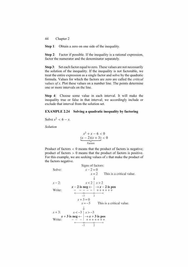
Step 1: Obtain a zero on one side of the inequality.

Step 2: Factor if possible. If the inequality is a rational expression,factor the numerator and the denominator separately.

Step 3: Set each factor equal to zero. These values are not necessarilythe solution of the inequality. If the inequality is not factorable, wetreat the entire expression as a single factor and solve by the quadraticformula. Values for which the factors are zero are called the criticalvalues of x. Plot these values on a number line. The points determineone or more intervals on the line.

Step 4: Choose some value in each interval. It will make theinequality true or false in that interval; we accordingly include orexclude that interval from the solution set.

EXAMPLE 2.24 Solving a quadratic inequality by factoring

Solve x2 < 6� x.

Solution

x2 C x � 6 < 0�x � 2�x C 3︸ ︷︷ ︸

Factors

< 0

Product of factors < 0 means that the product of factors is negative;product of factors > 0 means that the product of factors is positive.For this example, we are seeking values of x that make the product ofthe factors negative.

− − − − −Write: + + + + + +−3 2

x − 2 is neg ←

Signs of factors:x − 2 = 0

x = 2Solve:

This is a critical value.

x + 3 = 0x = −3 This is a critical value.

→ x − 2 is posx < 2x − 2: x > 2

Write:

x + 3:

− − − + + + + + + +−3 2

x + 3 is neg ← → x + 3 is posx < −3 x > −3

←

←

Chapter 2 45

We summarize these steps by writing

critical values →

← product of factors

neg.neg

pos posneg

neg.pos pos.pos

−3 2

− −− −

− − − + + + + ++ + + + + + + + +

We see from the number line that the segment labeled negativeis ��3, 2; this is the solution (except for a consideration of theendpoints). In this example, the endpoints are not included, so thesolution is an open interval. These steps are summarized as

posa b

pos ← sign of product (negative because of <)neg

− − − + + + ← signs of factors

�

EXAMPLE 2.25 Solving an inequality by examining the factors

Solve �2� x�x C 3�x � 1 ½ 0.

Solution Plotting critical values and checking the signs of the factors,we have

−3 1pos

+−− ++− +++ −++

posneg negEndpoints included because of ≥

2

The solution is ��1,�3] [ [1, 2]. �

EXAMPLE 2.26 Solving a rational inequality

Solvex C 3

x � 2< 0.

Solution Be careful not to multiply both sides by �x � 2, sincewe do not know whether �x � 2 is positive or negative. We couldconsider separate cases, but instead we solve the inequality as if it werequadratic. We set the numerator and denominator each equal to zeroto obtain the critical values x D �3, x D 2. We then plot these valueson a number line and check a value in each interval to determine thesolution.

−3− − + − + +

2

The solution is ��3, 2. �

46 Chapter 2

EXAMPLE 2.27 Solving a rational inequality

Solvex � 3

x> 1.

Solutionx � 3

x� 1 > 0

x � 3� xx

> 0

�3

x> 0

Since �3 < 0 for�3

x, we have

− − − +

0pos

x < 0 x > 0

neg

neg ÷ neg neg ÷ pos

The solution is ��1, 0. �

EXAMPLE 2.28 Solving a rational inequality

Solvex C 2

2x½ 5.

Solutionx C 2

2x� 5 ½ 0

x C 2� 10x

2x½ 0

2� 9x

2x½ 0

+ ÷ − + ÷ + − ÷ +

0 29pos negneg

The solution is �0, 29 ]. The endpoints are included when we have

intervals with ½ or �. However, values of the variable that causedivision by zero are excluded. �

Chapter 2 47

EXAMPLE 2.29 Solving a quadratic inequality that does notfactor

Solve x2 C 2x � 4 < 0.

Solution The left-hand expression is in simplified form and cannotbe factored. Therefore, we proceed by considering �x2 C 2x � 4 as asingle factor. To find the critical values, we find the values for whichthe factor is zero:

x2 C 2x � 4 D 0

x D �2šp4� 4�1��4

2

D �1šp

5

Next, we plot the critical values and check the sign of the expressionin each of the intervals:

+ +−

−1 − √5 −1 + √5

The solution is ��1�p5,�1Cp5. �

2.8 Determinants

Determinants are used in calculus in several places. We first seethem in Section 9.4 of the text, when they are used as memorydevices of an operation called the cross product. In Sections12.3 and 12.8, we use determinants to calculate what is calledthe Jacobian of a transformation. Finally, in Chapter 14, theWronskian is defined in terms of an nð n determinant.

The following arrays of numbers are examples of matrices:(a1 b1

a2 b2

)( a1 b1

a2 b2

a3 b3

)(a1 b1 c1 d1

a2 b2 c2 d2

)

The first of these matrices has two rows and two columns and is calleda ‘‘two-by-two matrix’’ (written ‘‘2ð 2 matrix’’), the second is a3ð 2 matrix, since it has three rows and two columns, and the lastone is a 2ð 4 matrix. The a’s, b’s, c’s, etc., that appear are called theentries of the matrix. An nð n matrix (i.e., a matrix with n rows andn columns, and hence a matrix with the same number of rows andcolumns) is called a square matrix. Associated with each square matrixis a certain number called the determinant of the matrix. We shallshow how to find the determinant of a 2ð 2 matrix and a 3ð 3 matrix.

48 Chapter 2

DETERMINANT

If A is the 2ð 2 matrix

[a bc d

], then the determinant of A

is defined to be the number ad� bc.

Some notations for this determinant are det A,

∣∣∣∣ a bc d

∣∣∣∣, and jAj. We

will generally use jAj.WARNING Note that determinants always have the same number of rowsand columns; that is, they are square: 2ð 2, 3ð 3, 4ð 4, Ð Ð Ð.EXAMPLE 2.30 Evaluating determinants

a.

∣∣∣∣ 4 �2�1 3

∣∣∣∣ D 4 Ð 3� ��2��1 D 12� 2 D 10

b.

∣∣∣∣ 2 22 2

∣∣∣∣ D 2 Ð 2� 2 Ð 2 D 0

c.

∣∣∣∣ 1 00 1

∣∣∣∣ D 1 Ð 1� 0 Ð 0 D 1

d.

∣∣∣∣ 1 22 4

∣∣∣∣ D 1 Ð 4� 2 Ð 2 D 0 �

We next define the determinant of a 3ð 3 matrix. We need apreliminary observation. If we delete the first row and first column ofthe matrix

A D[ a1 b1 c1

a2 b2 c2

a3 b3 c3

]

We obtain the 2ð 2 matrix

[b2 c2

b3 c3

]. This 2ð 2 matrix is referred to

as the minor associated with the entry in the first row and first column.Similarly, the minor associated with b1 is obtained by deleting the first

row and second column of A, and hence this minor is

[a2 c2

a3 c3

]. The

minor associated with c1 is

[a2 b2

a3 b3

]. The determinant of the 3ð 3

matrix A is obtained by using these minors as follows:

jAj D a1

∣∣∣∣ b2 c2

b3 c3

∣∣∣∣� b1

∣∣∣∣ a2 c2

a3 c3

∣∣∣∣C c1

∣∣∣∣ a2 b2

a3 b3

∣∣∣∣D a1

( minorassociated

with a1

)� b1

( minorassociated

with b1

)C c1

( minorassociated

with c1

)

Chapter 2 49

EXAMPLE 2.31 Evaluating a determinant∣∣∣∣∣1 4 �1�2 0 23 1 2

∣∣∣∣∣ D 1

∣∣∣∣ 0 21 2

∣∣∣∣� 4

∣∣∣∣�2 23 2

∣∣∣∣C ��1

∣∣∣∣�2 03 1

∣∣∣∣D �2C 4�10C 2 D 40 �

It is not difficult to show that

∣∣∣∣∣a 0 00 b 00 0 c

∣∣∣∣∣ D abc

We found the determinant for a 3ð 3 matrix by using the entries in thefirst row and their minors. In fact, it is possible to find the determinantusing any row (or column); the formulas are similar and use theminors of the terms in the given row (or column), but adjustmentsmust be made for the signs of the minors. The interested reader canfind these results in any standard college algebra book. The followingfour properties of determinants are worth noting:

HANDBOOK THEOREM 2 Properties of determinants

Property 1 If B is the matrix obtained from A by multi-plying a row (or column) of A by a realnumber k, then jBj D kjAj.

Property 2 If B is the matrix obtained from A by addingto a row (or column) of A a multiple of someother row (or column) of A, then jBj D jAj.

Property 3 If the matrix B is obtained from A byinterchanging two rows (or columns), thenjBj D �jAj.

Property 4 If two rows (or columns) of a matrix A areequal or proportional, then jAj D 0. �

EXAMPLE 2.32 Properties of determinants illustrated

a. Property 1:

∣∣∣∣ ka1 kb1

a2 b2

∣∣∣∣ D∣∣∣∣ a1 b1

ka2 kb2

∣∣∣∣ D k

∣∣∣∣ a1 b1

a2 b2

∣∣∣∣b. Property 2: Multiplying each entry in the first row of the matrix(

1 22 5

)D A by �2, and adding the result to the corresponding

entry in the second row, we obtain the matrix B D(

1 20 1

), and

property 2 asserts that jAj D jBj. (Check for yourself to see thatthis is correct.)

c. Property 3 (interchange the first and third rows):∣∣∣∣∣1 3 �53 �2 17 1 5

∣∣∣∣∣ D �∣∣∣∣∣7 1 53 �2 11 3 �5

∣∣∣∣∣

50 Chapter 2

d.

∣∣∣∣ 1 22 4

∣∣∣∣ D 0

Note that 2 times an entry in row 1 is equal to the correspondingentry in row 2. �

EXAMPLE 2.33 Multiplicative property of determinants

Verify that 2ð 2 determinants have the following multiplicativeproperty:∣∣∣∣ a1 b1

c1 d1

∣∣∣∣∣∣∣∣ a2 b2

c2 d2

∣∣∣∣ D∣∣∣∣ a1a2 C b1c2 a1b2 C b1d2

c1a2 C d1c2 c1b2 C d1d2

∣∣∣∣Solution∣∣∣∣ a1 b1

c1 d1

∣∣∣∣∣∣∣∣ a2 b2

c2 d2

∣∣∣∣ D �a1d1 � b1c1�a2d2 � b2c2

D a1a2d1d2 � b1c1a2d2 � a1d1b2c2 C b1b2c1c2

D �a1a2 C b1c2�c1b2 C d1d2� �a1b2 C b1d2�c1a2 C d1c2

D∣∣∣∣ a1a2 C b1c2 a1b2 C b1d2

c1a2 C d1c2 c1b2 C d1d2

∣∣∣∣ �

2.9 Functions

Definition: A function f is a rule that assigns, to each element x of aset X, a unique element y of a set Y. (See Section 1.3 of the text.)

In this handbook, we will simply list and categorize some of themore common types of functions you will encounter in calculus.

ALGEBRAIC FUNCTIONS:Definition: An algebraic function is a function that satisfies anequation of the form

an�xyn C an�1�xy

n�1 C Ð Ð Ð C a0�x D 0

where the coefficient functions ak�x are polynomials in x.

Polynomial Functions

Definition: f�x D anxn C an�1xn�1 C an�2xn�2 C Ð Ð Ð C a2x2 Ca1x C a0, an 6D 0

Constant function: f�x D a

Chapter 2 51

Linear function: f�x D ax C bStandard form: Ax C By CC D 0

Point-slope form: y � k D m�x � hSlope-intercept form: y D mx C bTwo-point form: y � y1 D

(y2 � y1

x2 � x1

)�x � x1 or∣∣∣∣∣

x y 1x1 y1 1x2 y2 1

∣∣∣∣∣ D 0

Intercept form:x

aC y

bD 1

Horizontal line: y D k

Vertical line: x D h

Quadratic function: f�x D ax2 C bx C c, a 6D 0Cubic function: f�x D ax3 C bx2 C cx C d, a 6D 0

Miscellaneous Algebraic Functions

Absolute value function: f�x D jxj D{

x if x ½ 0�x if x < 0

Greatest integer function: f�x D [[x]] This is the unique integer[[x]] satisfying [[x]] � x < [[x]]C 1; this means that [[x]] is the largestinteger not exceeding x. For example, [[2.3]] D 2, [[�2.3]] D �3, and[[2]] D 2.

Power function: f�x D xr for any real number r.

Rational function: f�x D P�x

D�x, where P�x and D�x are two

polynomial functions, with D�x 6D 0.

TRANSCENDENTAL FUNCTIONS:Definition: Functions that are not algebraic are called transcen-dental.

Exponential function: f�x D bx �b > 0, b 6D 1

Logarithmic function: f�x D logb x�b > 0, b 6D 1If b D 10, then f is a common logarithm: f�x D log xIf b D e, then f is a natural logarithm: f�x D ln x

52 Chapter 2

Trigonometric functions: Let ' be any angle in standard position,and let P�x, y be any point on the terminal side of the angle a distance

of r from the origin �r 6D 0. Then cos ' D x

r, sin ' D y

r, tan ' D y

x,

sec ' D r

x, csc ' D r

y, and cot ' D x

y.

2.10 Polynomials

THEOREMS Let P�x and Q�x be polynomial functions.

Zero factor theorem: If P�xQ�x D 0, then either P�x D 0 orQ�x D 0 (or both).

Remainder theorem: If P�x is divided by x � r until a constant isobtained, then the remainder is equal to P�r.

Intermediate-value theorem for a polynomial function: If P�xis a polynomial function on [a, b] such that P�a 6D P�b, then P takeson every value between P�a and P�b over the interval [a, b].

Factor theorem: If r is a root of the polynomial equation P�x D 0,then x � r is a factor of P�x. Also, if x � r is a factor of P(x), then ris a root of the polynomial equation P�x D 0.

Root limitation theorem: A polynomial function of degree n has,at most, n distinct roots.

Location theorem: If P is a polynomial function such that P�a andP�b are opposite in sign, then there is at least one real root on theinterval [a, b].

Rational root theorem: If P�x has integer coefficients and has arational root p/q (where p/q is reduced), then p is a factor of theconstant term, a0, and q is a factor of the leading coefficient, an.

Upper and lower bound theorem: If a > 0 and, in the syntheticdivision of P�x by x � a, all the numbers in the last row are eitherpositive or negative, then a is an upper bound for the roots ofP�x D 0.If b < 0 and, in the synthetic division of P�x by x � b, the numbersin the last row alternate in sign, then b is a lower bound for the rootsof P�x D 0.

Descartes’s rule of signs: Let P�x be written in descending powersof x. Then

1. The number of positive real zeros is equal to the number of signchanges or is equal to that number decreased by an even integer.

Chapter 2 53

2. The number of negative real zeros is equal to the number of signchanges in P��x or is equal to that number decreased by aneven integer.

Fundamental theorem of algebra: If P�x is a polynomial ofdegree n ½ 1 with complex coefficients, then P�x D 0 has at leastone complex root.

Number-of-roots theorem: If P�x is a polynomial of degree n ½ 1with complex coefficients, then P�x D 0 has exactly n roots (if rootsare counted according to their multiplicity).

EXAMPLE 2.34 Synthetic division

Divide x4 C 3x3 � 12x2 C 5x � 2 by x � 2.

Solution To do synthetic division, the divisor must be of the formx � b.

This is the number b.# 1 3 �12 5 �2 Coefficients of2j 2Ł 10 �4 2 given polynomial

1 5 �2 1 0" "

— Add "Remainder

Bring down leading coefficient

ŁThe numbers in this row are found as follows:

2 Р1 D 2; 2 Р5 D 10; 2 Р��2 D �4; 2 Р1 D 2

The degree of the result is one less than the degree of the givenpolynomial and has coefficients given by the last row (1, 5, �2, and 1for this example; the last entry is the remainder). Thus,

x4 C 3x3 � 12x2 C 5x � 2

x � 2D x3 C 5x2 � 2x C 1 �

EXAMPLE 2.35 Synthetic division with zero coefficients and aremainder

Divide x5 � 3x2 C 1 by x � 2.

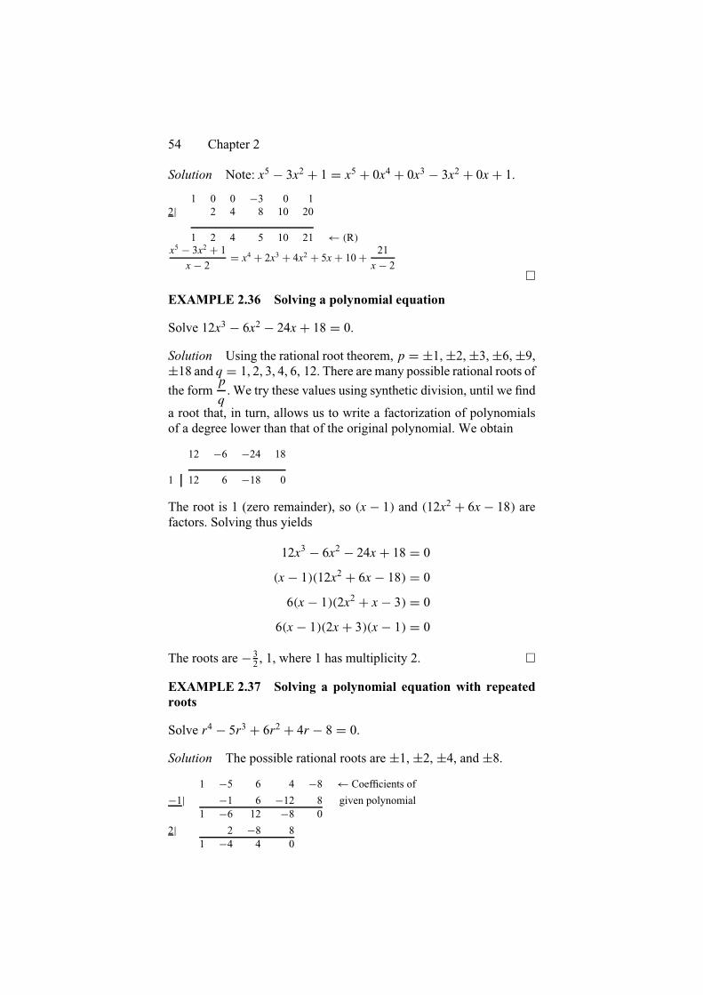
54 Chapter 2

Solution Note: x5 � 3x2 C 1 D x5 C 0x4 C 0x3 � 3x2 C 0x C 1.

1 0 0 �3 0 12j 2 4 8 10 20

1 2 4 5 10 21 �Rx5 � 3x2 C 1

x � 2D x4 C 2x3 C 4x2 C 5x C 10C 21

x � 2�

EXAMPLE 2.36 Solving a polynomial equation

Solve 12x3 � 6x2 � 24x C 18 D 0.

Solution Using the rational root theorem, p D š1,š2,š3,š6,š9,š18 and q D 1, 2, 3, 4, 6, 12. There are many possible rational roots of

the formp

q. We try these values using synthetic division, until we find

a root that, in turn, allows us to write a factorization of polynomialsof a degree lower than that of the original polynomial. We obtain

12 �6 �24 18

1 12 6 �18 0

The root is 1 (zero remainder), so �x � 1 and �12x2 C 6x � 18 arefactors. Solving thus yields

12x3 � 6x2 � 24x C 18 D 0

�x � 1�12x2 C 6x � 18 D 0

6�x � 1�2x2 C x � 3 D 0

6�x � 1�2x C 3�x � 1 D 0

The roots are � 32 , 1, where 1 has multiplicity 2. �

EXAMPLE 2.37 Solving a polynomial equation with repeatedroots

Solve r4 � 5r3 C 6r2 C 4r � 8 D 0.

Solution The possible rational roots are š1, š2, š4, and š8.

1 �5 6 4 �8 Coefficients of

�1j �1 6 �12 8 given polynomial1 �6 12 �8 0

2j 2 �8 81 �4 4 0

Chapter 2 55

Solving the remaining quadratic:

x2 � 4x C 4 D 0

�x � 22 D 0

x D 2

The roots are �1 and 2. Note: The root 2 has multiplicity 3. �

EXAMPLE 2.38 Solving a polynomial equation that has norational roots

Solve x4 � 3x2 � 6x � 2 D 0.

Solution p: š1, š2 and q: 1, sop

q: š1,š2. We try these values,

using synthetic division:

1 0 �3 �6 �21 1 1 �2 �8 �10

2 1 2 1 �4 �10�1 1 �1 �2 �4 2�2 1 �2 1 �8 14 Lower bound

There are no rational roots. (We have tried all the numbers on ourlist.) Next, we verify the type of roots by using Descartes’s rule ofsigns. First,

f�x D x4 � 3x2 � 6x � 2

There is one sign change, so there is one positive root. Next,

f��x D x4 � 3x2 C 6x � 2

There are three sign changes, so we have three negative roots or onenegative root.

Using synthetic division to find some additional points yields

�0,�2 for the y-intercept;

�1.5,�12.6875;

�3, 34; there are no roots larger than 3

Using the intermediate-value theorem and synthetic division, we canfind the roots to any desired degree of accuracy. We find the following:

56 Chapter 2

1 0 �3 �6 �2�0.5 1 �0.5 �2.75 �4.625 0.3125�0.4 1 �0.4 �2.84 �4.864 �0.0544�0.41 1 �0.41 �2.8319 �4.8389 �0.0161�0.42 1 �0.42 �2.8236 �4.8141 0.0219

Remember that there is a root between �0.41 and �0.42, since theremainder is positive for �0.42 and negative for �0.41. We continuein this fashion to approximate the root to any degree of accuracydesired. This is a good problem for a calculator or a computer. Werepeat the procedure for the other roots to find (correct to the nearesttenth) �0.4, 2.4. The graph can be used to verify that these are theonly real roots. �

You may need to consult a precalculus textbook for a review of howto solve polynomial equations.

2.11 PROBLEM SET 2

Perform the indicated operations in Problems 1–12.

1. 25 Ð 27 2. 52 Ð 58 3. �523 4. �824

5.38

356.

35

387. 2�5 Ð 28 8.

2�5

28

9.2�3

2�410. 82/3 Ð 41/2 11. 163/4 Ð 8�1/3 12.

82/3

41/2

Perform the indicated operations Problems 13–22. Assume that a,b, and c are positive real numbers.

13. �a2b3c5 Ð �a3b5c2 14. �a2b3c5 Ð �a�2b�4c�2

15. �ab2c34 16.(a2b3

c2

)5

17.(a�2b2

c2

)�1

18.(a�2b�2

c2

)�1

19.(a�2b�2

c�2

)�2

20. x�2 C y�2

21. �x�2 C y�2�2 22. �a1/2b2/3c1/515

Factor the expressions in Problems 23–32.

23. 2a1/2b�1/2 C 3a�1/2b1/2 24. �3a�1/2bC 4a1/2

25. a1/2bC a�1/2b2 26. a1/2b�1/3 C a�1/2b1/3

27. �x � 124 � 2�x � 12(Adapted from Problem 20, Section 4.3, of text.)

Chapter 2 57

28. 12u3 � 6u2 � 24u(Adapted from Problem 22, Section 4.3, of text.)

29. 2x�2x C 32 C 2x2�2x C 3�2(Adapted from Problem 42, Section 3.5, of text.)

30. [2x]�4x C 53 C x2[3�4x C 52�4](From Example 9, Section 3.5, of text.)

31. �x C 13�2�2x C 3�2C �2x C 32�3�x C 12�132. 4�2x2 C 13�4x�x2 � 25 C 5�2x2 C 14�2x�x2 � 24

In Problems 33–58, solve each equation or inequality for x.

33. 3x � 9 ½ 12 34. �x > �3635. 3�2� 4x � 0 36. 5�3� x > 3x � 137. �5 � 5x � 25 38. 3 � �x < 839. �5 < 3x C 2 � 5 40. �5 � 3� 2x < 1841. x2 C 5x � 6 D 0 42. x2 C 5x C 6 D 043. 3x2 D 7x 44. 7x2 D 245. 5x D 3� 4x2 46. 4x2 D 12x � 947. 2x2 C x � w D 0 48. 2x2 C wx C 5 D 049. 4x2 � 4x C �1� t2 D 0 50. y D 2x2 C x C 651. 4x2 � �3t C 10x C �6t C 4 D 0, t > 252. �x � 32 C �y � 22 D 453. �x C 1�2x C 5�7� 3x > 054. �x � 2�3x C 2�3� 2x < 0

55.x�2x � 1

5� x > 0 56.x

�2x C 3�x � 2< 0

57. 2x2 C 4x C 5 ½ 0 58. x2 � 2x � 6 � 0

In Problems 59–70, find the value of the given determinant.

59.

∣∣∣∣∣∣3 0 0�5 2 05

2

1

5�1

∣∣∣∣∣∣ 60.

∣∣∣∣∣0 1 0�1 32 12 48 �1

∣∣∣∣∣61.

∣∣∣∣∣2 0 11 3 �22 �3 2

∣∣∣∣∣ 62.

∣∣∣∣∣0 �1 �11 3 21 �4 2

∣∣∣∣∣63.

∣∣∣∣∣�1 1 20 1 31 0 �1

∣∣∣∣∣ 64.

∣∣∣∣∣2 �1 11 0 00 �1 2

∣∣∣∣∣65.

∣∣∣∣∣1 �2 3�4 7 �115 9 �1

∣∣∣∣∣ 66.

∣∣∣∣∣i j k2 �1 30 7 �4

∣∣∣∣∣(From Example 5, For variables i, j, and k.

Section 9.4, of text.) (From Example 1, Section 9.4, of text.)

58 Chapter 2

67.

∣∣∣∣∣1 2 30 0 10 1 0

∣∣∣∣∣ 68.

∣∣∣∣∣2 3 42 0 00 1 1

∣∣∣∣∣69.

∣∣∣∣∣∣∣1 2 3 48 �1 5 72 4 6 8�1 5 3 7

∣∣∣∣∣∣∣ 70.

∣∣∣∣∣∣∣8 1 �7 5�1 2 2 3�7 8 15 4�3 6 6 9

∣∣∣∣∣∣∣In Problems 71–76, expand the given quantity.

71. �aC b4 72. �aC 2b3 73. �3x C 2y3

74. ��x C 2y5 75. �1

xC y4 76. �

paC 2b5

Solve the polynomial equations in Problems 77–90.

77. x3 � x2 � 4x C 4 D 078. 2x3 � x2 � 18x C 9 D 079. x3 � 2x2 � 9x C 18 D 080. x3 C 2x2 � 5x � 6 D 081. x3 C 3x2 � 4x � 12 D 082. 2x3 C x2 � 13x C 6 D 083. 2x3 � 3x2 � 32x � 15 D 084. x4 � 12x3 C 54x2 � 108x C 81 D 085. x4 C 3x3 � 19x2 � 3x C 18 D 086. x4 � 13x2 C 36 D 087. x3 C 15x2 C 71x C 105 D 088. x5 C 6x4 C x3 � 48x2 � 92x � 48 D 089. x6 � 3x4 C 3x2 � 1 D 090. x7 C 3x6 � 4x5 � 16x4 � 13x3 � 3x2 D 091. Evaluate the determinant∣∣∣∣∣

sin* cos ' �+ sin* sin ' + cos* cos 'sin* sin ' + sin* cos ' + cos* sin '

cos* 0 �+ sin*

∣∣∣∣∣This problem is from Example 6 of Section 12.8